Large-Sample Confidence Intervals for a Mean
Many important engineering applications of statistics fit the following standard mold. Values for parameters of a data-generating process are unknown. Based on data, the object is
- identify an interval of values likely to contain an unknown parameter (or a function of one or more parameters) and
- quantify “how likely” the interval is to cover the correct value.
.
For example, a piece of equipment that dispenses baby food into jars might produce an unknown mean fill level, µ. Determining a data-based interval likely to contain µ and an evaluation of the reliability of the interval might be important. Or a machine that puts threads on U-bolts might have an inherent variation in thread lengths, describable in terms of a standard deviation, σ . The point of data collection might then be to produce an interval of likely values for σ , together with a statement of how reliable the interval is. Or two different methods of running a pelletizing machine might have different unknown propensities to produce defective pellets, (say, p1 and p2). A data-based interval for p1 − p2 , together with an associated statement of reliability, might be needed
.
DEFINITION 5.1.1.1 Confidence Interval
A confidence interval for a parameter (or function of one or more parameters) is a data-based interval of numbers thought likely to contain the parameter (or function of one or more parameters) possessing a stated probability-based confidence or reliability.
This section discusses how basic probability facts lead to simple large-sample formulas for confidence intervals for a mean, µ. The unusual case where the standard deviation σ is known is treated first. Then parallel reasoning produces a formula for the much more common situation where σ is not known. The section closes with discussions of three practical issues in the application of confidence intervals.
A Large-n Confidence Interval for  involving
The final example in Chapter 4.2.2.4 involved a physically stable filling process known to have a net weight standard deviation of σ = 1.6 g. Since, for large n,thesample mean of iid random variables is approximately normal, the final example of Chapter 4.2.4 argued that for n = 47 and
 = the sample mean net fill weight of 47 jars filled by the process (g)
here is an approximately 80% chance that is within .3 gram of µ. This fact is pictured again in Figure 5.1.1.1.

Figure 5.1.1.1 Approximate probability distribution for x¯ based on n = 47
Notation ConventionsWe need to interrupt for a moment to discuss notation. In Part 4, capital letters were carefully used as symbols for random variables and corresponding lowercase letters for their possible or observed values. But here a lowercase symbol, has been used for the sample mean random variable. This is fairly standard statistical usage, and it is in keeping with the kind of convention used in earlier Parts. We are thus going to now abandon strict adherence to the capitalization convention introduced in Chapter 4. Random variables will often be symbolized using lowercase letters and the same symbols used for their observed values. The Chapter 4 capitalization convention is especially helpful in learning the basics of probability. But once those basics are mastered, it is common to abuse notation and to determine from context whether a random variable or its observed value is being discussed.
.
The most common way of thinking about a graphic like Figure 5.1.1.1 is to think of the possibility that
5.1.1.1 
in terms of whether or not falls in an interval of length 2(.3) = .6 centered at µ. But the equivalent is to consider whether or not an interval of length .6 centered at falls on top of µ. Algebraically, inequality (5.1.1.1) is equivalent to
5.1.1.2 
which shifts attention to this second way of thinking. The fact that expression (5.1.1.2) has about an 80% chance of holding true anytime a sample of 47 fill weights is taken suggests that the random interval
5.1.1.3 ")
can be used as a confidence interval for µ, with 80% associated reliability or confidence.
Suppose a sample of n = 47 jars produces = 138.2 g. Then expression (5.1.1.3) suggests that the interval with endpoints
138.2 g  .3 g
.3 g
(i.e., the interval from 137.9 g to 138.5 g) be used as an 80% confidence interval for the process mean fill weight.
It is not hard to generalize the logic that led to expression (5.1.1.3). Anytime an iid model is appropriate for the elements of a large sample, the central limit theorem implies that the sample mean is approximately normal with mean µ and standard deviation σ/√n. Then, if for p >.5, z is the p quantile of the standard normal distribution, the probability that
5.1.1.4 
is approximately 1 − 2(1 − p). But inequality (5.1.1.4) can be rewritten as
5.1.1.5 
and thought of as the eventuality that the random interval with endpoints
EXPRESSION 5.1.1.6 Large-Sample Known Confidence Limits for

brackets the unknown µ. So an interval with endpoints (5.1.1.6) is an approximate confidence interval for µ (with confidence level 1 − 2(1 − p)).
In an application, z in equation (5.1.1.6) is chosen so that the standard normal probability between −z and z corresponds to a desired confidence level. Apendix Table A1.1 (of standard normal cumulative probabilities) can be used to verify the appropriateness of the entries in Table 5.1.1.1. (This table gives values of z for use in expression (5.1.1.6) for some common confidence levels.)

Table 5.1.1.1
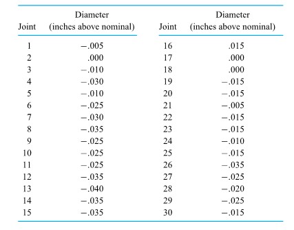
Dib, Smith, and Thompson studied a grinding process used in the rebuilding of automobile engines. The natural short-term variability associated with the diameters of rod journals on engine crankshafts ground using the process was on the order of σ = .7 × 10−4 in. Suppose that the rod journal grinding process can be thought of as physically stable over runs of, say, 50 journals or less. Then if 32 consecutive rod journal diameters have mean deviation from nominal of =−.16 × 10−4 in., it is possible to apply expression (5.1.1.6) to make a confidence interval for the current process mean deviation from nominal. Consider a 95% confidence level. Consulting Table 5.1.1.1 (or otherwise, realizing that 1.96 is the p =.975 quantile of the standard normal distribution), z = 1.96 is called for in formula (5.1.1.6) (since .95 = 1 − 2(1 − .975)). Thus, a 95% confidence interval for the current process mean deviation from nominal journal diameter has endpoints
 \frac{.7 \times 10^{-4}}{\sqrt{32}}")
that is, endpoints

An interval like this one could be of engineering importance in determining the advisability of making an adjustment to the process aim. The interval includes both positive and negative values. So although < 0, the information in hand doesn’t provide enough precision to tell with any certainty in which direction the grinding process should be adjusted. This, coupled with the fact that potential machine adjustments are probably much coarser than the best-guess misadjustment of =−.16 × 10−4 in., speaks strongly against making a change in the process aim based on the current data.
A Generally Applicable Large-n Confidence Interval for
Although expression (5.1.1.6) provides a mathematically correct confidence interval, the appearance of σ in the formula severely limits its practical usefulness. It is unusual to have to estimate a mean µ when the corresponding σ is known (and can therefore be plugged into a formula). These situations occur primarily in manufacturing situations like those of Examples 5.1.1.1 and 2. Considerable past experience can sometimes give a sensible value for σ , while physical process drifts over time can put the current value of µ in question.
Happily, modification of the line of reasoning that led to expression (5.1.1.1) produces a confidence interval formula for µ that depends only on the characteristics of a sample. The argument leading to formula (5.1.1.6) depends on the fact that for large n, is approximately normal with mean µ and standard deviation σ/√n—i.e., that
5.1.1.7 
is approximately standard normal. The appearance of σ in expression (5.1.1.7) is what leads to its appearance in the confidence interval formula (5.1.1.6). But a slight generalization of the central limit theorem guarantees that for large n,
5.1.1.8 
is also approximately standard normal. And the variable (5.1.1.8) doesn’t involve σ .
Beginning with the fact that (when an iid model for observations is appropriate and n is large) the variable (5.1.1.8) is approximately standard normal, the reasoning is much as before. For a positive z,
-z <  < z
< z
is equivalent to

which in turn is equivalent to

Thus, the interval with random center and random length 2zs/√n—i.e., with random endpoints
EXPRESSION 5.1.1.9 Large-Sample Confidence Levels for

can be used as an approximate confidence interval for µ. For a desired confidence, z should be chosen such that the standard normal probability between −z and z corresponds to that confidence level.
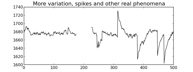
F. Willett, in the article “The Case of the Derailed Disk Drives” (Mechanical Engineering, 1988), discusses a study done to isolate the cause of “blink code A failure” in a model of Winchester hard disk drive. Included in that article are the data given in Figure 5.1.1.2. These are breakaway torques (units are inch ounces) required to loosen the drive’s interrupter flag on the stepper motor shaft for 26 disk drives returned to the manufacturer for blink code A failure. For these data, = 11.5 in. oz and s = 5.1 in. oz.
If the disk drives that produced the data in Figure 5.1.1.2 are thought of as representing the population of drives subject to blink code A failure, it seems reasonable to use an iid model and formula (5.1.1.9) to estimate the population mean breakaway torque. Choosing to make a 90% confidence interval for µ, z = 1.645
is indicated in Table 5.1.1.1. And using formula (5.1.1.9), endpoints

(i.e., endpoints 9.9 in. oz and 13.1 in. oz) are indicated.
The interval shows that the mean breakaway torque for drives with blink code A failure was substantially below the factory’s 33.5 in. oz target value. Recognizing this turned out to be key in finding and eliminating a design flaw in the drives.
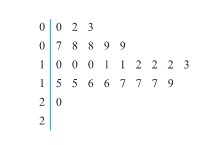
Figure 5.1.1.2 Torques required to loosen 26 interrupter flags
C: Some Comments Concerning Confidence Intervals
Formulas (5.1.1.6) and (5.1.1.9) have been used to make confidence statements of the type “µ is between a and b.” But often a statement like “µ is at least c”or“µ is no more than d ” would be of more practical value. For example, an automotive engineer might wish to state, “The mean NO emission for this engine is at most 5 ppm.” Or a civil engineer might want to make a statement like “the mean compressive strength for specimens of this type of concrete is at least 4188 psi.” That is, practical engineering problems are sometimes best addressed using one-sided confidence intervals.
Making one-sided confidence intervalsThere is no real problem in coming up with formulas for one-sided confidence intervals. If you have a workable two-sided formula, all that must be done is to
1. replace the lower limit with −∞ or the upper limit with +∞ and
2. adjust the stated confidence level appropriately upward (this usually means
dividing the “unconfidence level” by 2).
This prescription works not only with formulas (5.1.1.6) and (5.1.1.9) but also with the rest of the two-sided confidence intervals introduced in this chapter.
For the mean breakaway torque for defective disk drives, consider making a one-sided 90% confidence interval for µ of the form (−∞, #), for # an appropriate number. Put slightly differently, consider finding a 90% upper confidence bound for µ,(say,#).’
Beginning with a two-sided 80% confidence interval for µ, the lower limit canbe replaced with −∞ and a one-sided 90% confidence interval determined. Thatis, using formula (6.9), a 90% upper confidence bound for the mean breakaway torque is

Equivalently, a 90% one-sided confidence interval for µ is (−∞, 12.8).
The 12.8 in. oz figure here is less than (and closer to the sample mean than) the 13.1 in. oz upper limit from the 90% two-sided interval found earlier. In the one-sided case, −∞ is declared as a lower limit so there is no risk of producing an interval containing only numbers larger than the unknown µ. Thus an upper limit smaller than that for a corresponding two-sided interval can be used.
Interpreting a confidence interval
A second issue in the application of confidence intervals is a correct understanding of the technical meaning of the term confidence. Unfortunately, there are many possible misunderstandings. So it is important to carefully lay out what confidence
does and doesn’t mean.
Prior to selecting a sample and plugging into a formula like (5.1.1.6) or (5.1.1.9), the meaning of a confidence level is obvious. Choosing a (two-sided) 90% confidence level and thus z = 1.645 for use in formula (5.1.1.9), before the fact of sample selection and calculation, “there is about a 90% chance of winding up with an interval that brackets µ.” In symbols, this might be expressed as
![P\left[\bar{x}-1.645 \frac{s}{\sqrt{n}}<\mu<\bar{x}+1.645 \frac{s}{\sqrt{n}}\right] \approx .90](https://atu0g9ctah.execute-api.ca-central-1.amazonaws.com/latest/latex?latex=P%5Cleft%5B%5Cbar%7Bx%7D-1.645%20%5Cfrac%7Bs%7D%7B%5Csqrt%7Bn%7D%7D%3C%5Cmu%3C%5Cbar%7Bx%7D%2B1.645%20%5Cfrac%7Bs%7D%7B%5Csqrt%7Bn%7D%7D%5Cright%5D%20%5Capprox%20.90&fg=000000&font=TeX&svg=1 "P\left[\bar{x}-1.645 \frac{s}{\sqrt{n}}<\mu<\bar{x}+1.645 \frac{s}{\sqrt{n}}\right] \approx .90")
But how to think about a confidence level after sample selection? This is an entirely different matter. Once numbers have been plugged into a formula like (5.1.1.6) or (5.1.1.9), the die has already been cast, and the numerical interval is either right or wrong. The practical difficulty is that while which is the case can’t be determined, it no longer makes logical sense to attach a probability to the correctness of the interval. For example, it would make no sense to look again at the two-sided interval found in Example 5.1.1.3 and try to say something like “there is a 90% probability that µ is between 9.9 in. oz and 13.1 in. oz.” µ is not a random variable. It is a fixed (although unknown) quantity that either is or is not between 9.9 and 13.1. There is no probability left in the situation to be discussed.
So what does it mean that (9.9, 13.1) is a 90% confidence interval for µ? Like it or not, the phrase “90% confidence” refers more to the method used to obtain the interval (9.9, 13.1) than to the interval itself. In coming up with the interval, methodology has been used that would produce numerical intervals bracketing µ in about 90% of repeated applications. But the effectiveness of the particular interval in this application is unknown, and it is not quantifiable in terms of a probability. A person who (in the course of a lifetime) makes many 90% confidence intervals can expect to have a “lifetime success rate” of about 90%. But the effectiveness of any particular application will typically be unknown.
A short statement summarizing this discussion as “the interpretation of confidence” will be useful.
DEFINITION 5.1.1.2 Interpretation of a Confidence Interval
To say that a numerical interval (a, b) is (for example) a 90% confidence interval for a parameter is to say that in obtaining it, one has applied methods of data collection and calculation that would produce intervals bracketing the parameter in about 90% of repeated applications. Whether or not the particular interval (a, b) brackets the parameter is unknown and not describable in terms of a probability.
The reader may feel that the statement in Definition 5.1.1.2 is a rather weak meaning for the reliability figure associated with a confidence interval. Nevertheless, the statement in Definition 5.1.1.2 is the correct interpretation and is all that can be rationally expected. And despite the fact that the correct interpretation may initially seem somewhat unappealing, confidence interval methods have proved themselves to be of great practical use.
D: Sample Sizes for estimating
As a final consideration in this introduction to confidence intervals, note that formulas like (5.1.1.6) and (5.1.1.9) can give some crude quantitative answers to the question, “How big must n be?” Using formula (5.1.1.9), for example, if you have in mind (1) a desired confidence level, (2) a worst-case expectation for the sample standard deviation, and (3) a desired precision of estimation for µ, it is a simple matter to solve for a corresponding sample size. That is, suppose that the desired confidence level dictates the use of the value z in formula (5.1.1.9), s is some likely worst-case value for the sample standard deviation, and you want to have confidence limits (or a limit) of the form ±  . Setting

and solving for n produces the requirement
^2")
Suppose that in the disk drive problem, engineers plan to follow up the analysis of the data in Figure 5.1.1.2 with the testing of a number of new drives. This will be done after subjecting them to accelerated (high) temperature conditions, in an effort to understand the mechanism behind the creation of low breakaway torques. Further suppose that the mean breakaway torque for temperature-stressed drives is to be estimated with a two-sided 95% confidence interval and that the torque variability expected in the new temperature-stressed drives is no worse than the s = 5.1 in. oz figure obtained from the returned drives. A ±1 in. oz precision of estimation is desired. Then using the plus-or-minus part of formula (5.1.1.9) and remembering Table 5.1.1.1, the requirement is

which, when solved for n, gives
(5.1)}{1}\right)^2 \approx 100")
A study involving in the neighborhood of n = 100 temperature-stressed new disk drives is indicated. If this figure is impractical, the calculations at least indicate that dropping below this sample size will (unless the variability associated with the stressed new drives is less than that of the returned drives) force a reduction in either the confidence or the precision associated with the final interval.
For two reasons, the kind of calculations in the previous example give somewhat less than an ironclad answer to the question of sample size. The first is that they are only as good as the prediction of the sample standard deviation, s. If s is underpredicted, an n that is not really large enough will result. (By the same token, if one is excessively conservative and overpredicts s, an unnecessarily large sample size will result.) The second issue is that expression (5.1.1.9) remains a large-sample formula. If calculations like the preceding ones produce n smaller than, say, 25 or 30, the value should be increased enough to guarantee that formula (5.1.1.9) can be applied.


 =
= 
 in free fall an object will have velocity
 =
= 

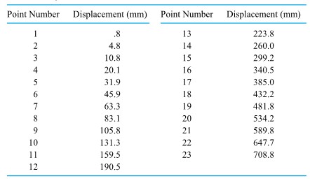
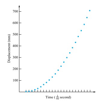
 of a second. Table 1.1.7.1 gives measurements of such positions. (Dr. Frank Peterson of the ISU Physics and Astronomy Department supplied the tape.) Plotting the bob positions in the table at equally spaced intervals produces the approximately quadratic plot shown in Figure 1.1.7.2. Picking a parabola to fit the plotted points involves identifying an appropriate value for
  /
/ , not far from the commonly quoted value of 9.8

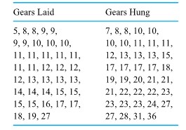
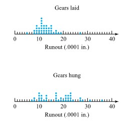
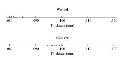
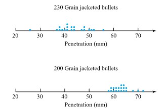
 from the target surface to the back of the bullets) for two bullet types. Figure 2.2.2.2 presents a corresponding pair of dot diagrams.
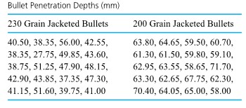

 ” and ”
  ” leaf positions for each possible leading digit, instead of only a single ”
  ” leaf for each leading digit.


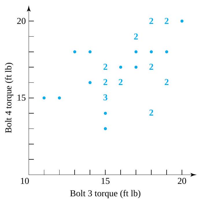
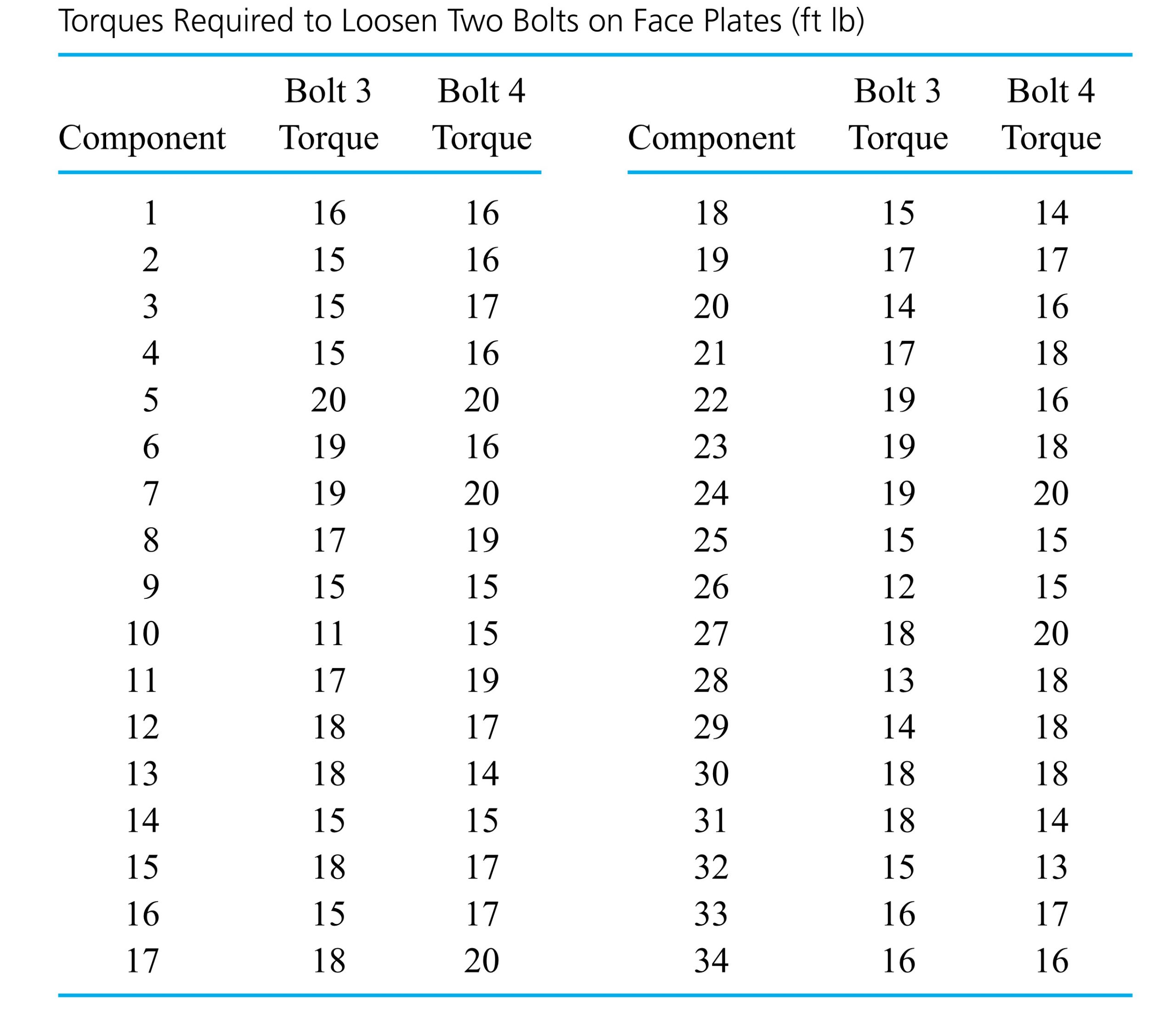
 required for bolts number 3 and 4), respectively, on 34 different components. Figure 2.1.4.1 is a scatterplot of the bivariate data from Table 2.1.4.1. In this figure, where several points must be plotted at a single location, the number of points occupying the location has been plotted instead of a single dot.

 of those taking the test had worse scores, and roughly
  had better scores. This concept is also useful in the description of engineering data. However, because it is often more convenient to work in terms of fractions between 0 and 1 rather than in percentages between 0 and 100, slightly different terminology will be used here: “Quantiles,” rather than percentiles, will be discussed. After the quantiles of a data set are carefully defined, they are used to create a number of useful tools of descriptive statistics: quantile plots, boxplots,
  plots, and normal plots (a type of theoretical
  between 0 and 1 , the
  of the distribution lies to the right. However, because of the discreteness of finite data sets, it is necessary to state exactly what will be meant by the terminology. Definition 1 gives the precise convention that will be used in this text.
 values that when ordered are
  ,
, for a positive integer
  , the
, the =Q\left(\frac{i-.5}{n}\right)=x_{i}")
 quantile.)
 and
and  that is not of the form
  , the
, the ") with corresponding
with corresponding ") will be used to denote the
will be used to denote the  and
and  / n") . To find
. To find  / n") for
for 
") th ordered data point.”
th ordered data point.” , one can easily find the
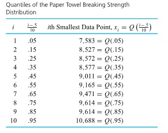
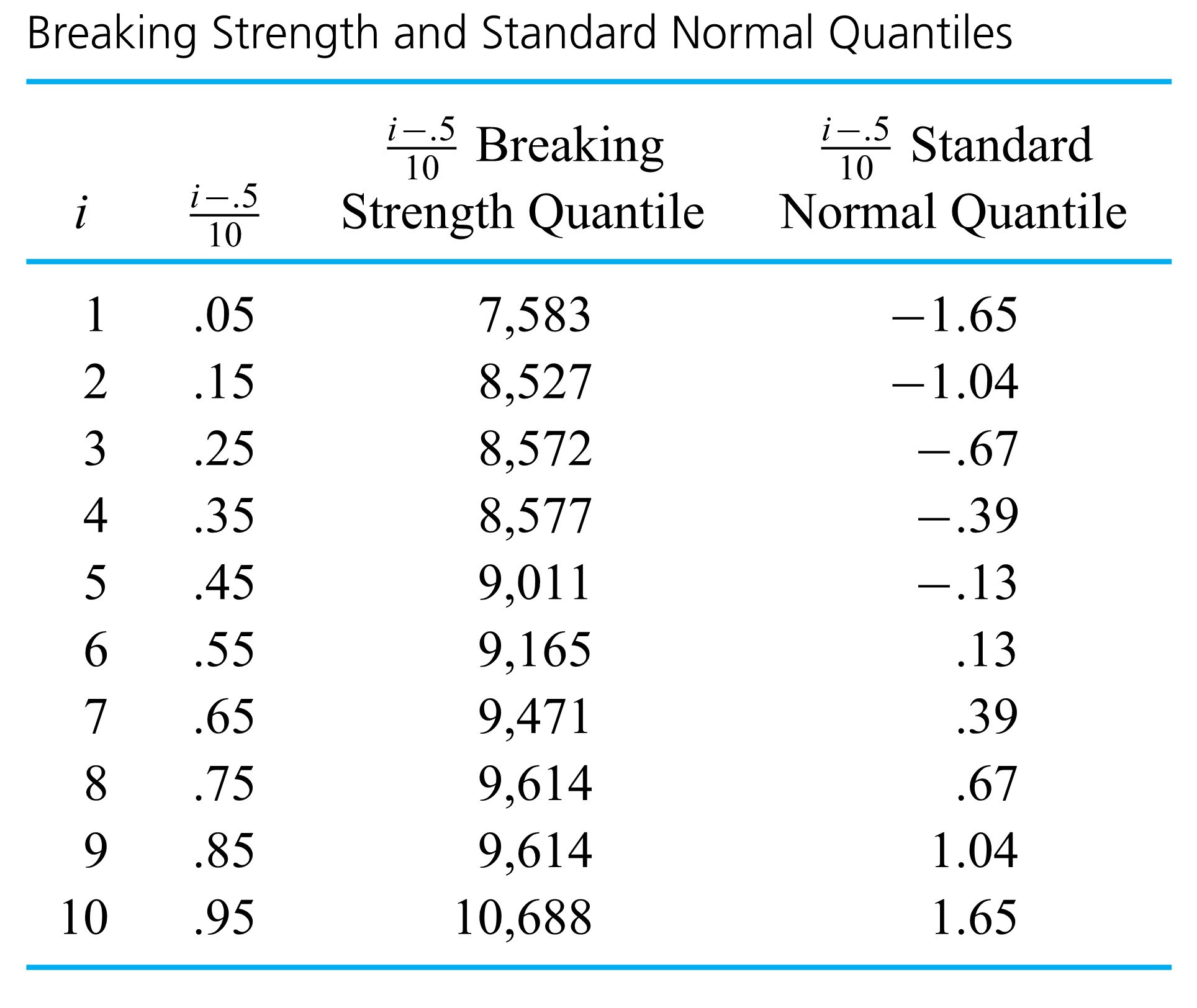
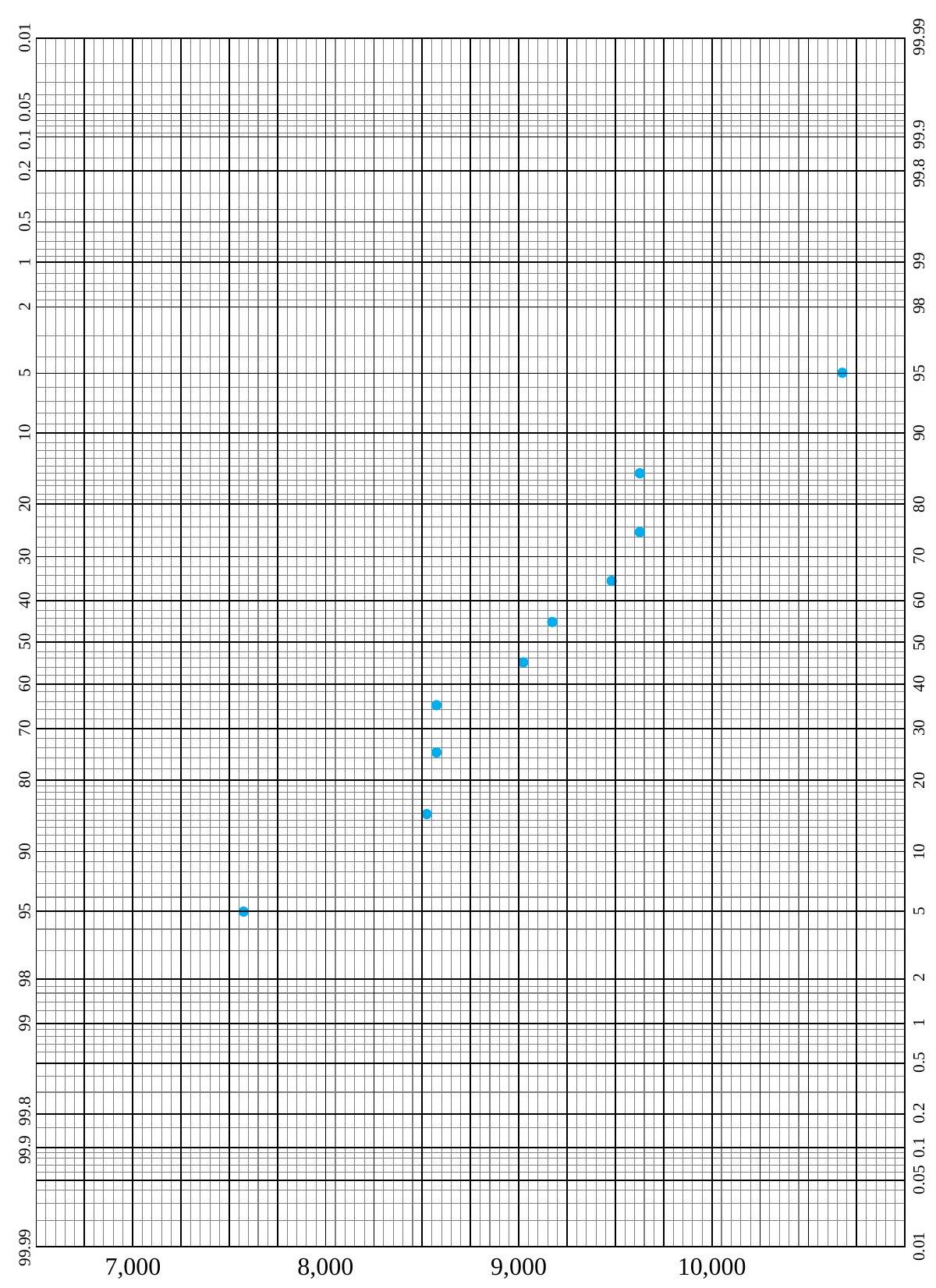
  , and .95 quantiles of the breaking strength distribution, as shown in Table 31.5.2.
 data points, each one accounts for
  of the data set. Applying convention (1) in Definition 3.1.5.1 to find (for example) the .35 quantile, the smallest 3 data points and half of the fourth smallest are counted as lying to (continued) the left of the desired number, and the largest 6 data points and half of the seventh largest are counted as lying to the right. Thus, the fourth smallest data point must be the .35 quantile, as is shown in Table 2.1.5.2.
 of the way from .45 to .55 , linear interpolation gives:
=(1-.5) Q(.45)+.5 Q(.55)=.5(9,011)+.5(9,165)=9,088 \mathrm{~g}")
 of the way from .85 to .95 , linear interpolation gives:
=(1-.8) Q(.85)+.8 Q(.95)=.2(9,614)+.8(10,688)=10,473.2 \mathrm{~g}")
") is called the median of a distribution.
is called the median of a distribution.") and
and ") are called the first (or lower) quartile and third (or upper) quartile of a distribution, respectively.
are called the first (or lower) quartile and third (or upper) quartile of a distribution, respectively.") previously computed, for the (continued) breaking strength distribution
previously computed, for the (continued) breaking strength distribution=9,088 \mathrm{~g} \\\text { 1st quartile } & =Q(.25)=8,572 \mathrm{~g} \\\text { 3rd quartile } & =Q(.75)=9,614 \mathrm{~g}\end{aligned}")
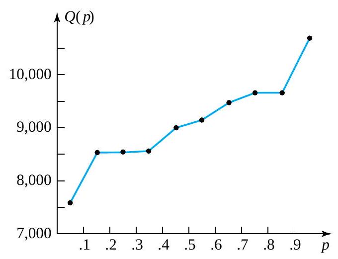
") and then connecting consecutive plotted points with straight-line segments.
and then connecting consecutive plotted points with straight-line segments.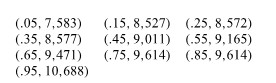
-Q(.25)")
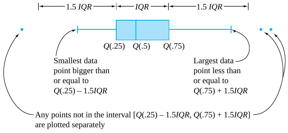
") and the largest data point within 1.5IQR of
and the largest data point within 1.5IQR of ![[Q(.25)-1.5 I Q R, Q(.75)+1.5 I Q R]](https://atu0g9ctah.execute-api.ca-central-1.amazonaws.com/latest/latex?latex=%5BQ%28.25%29-1.5%20I%20Q%20R%2C%20Q%28.75%29%2B1.5%20I%20Q%20R%5D&fg=000000&font=TeX&svg=1 "[Q(.25)-1.5 I Q R, Q(.75)+1.5 I Q R]") . Any that are not then get plotted individually and are thereby identified as outlying or unusual.
. Any that are not then get plotted individually and are thereby identified as outlying or unusual. & =8,572 \mathrm{~g} \\Q(.5) & =9,088 \mathrm{~g} \\Q(.75) & =9,614 \mathrm{~g}\end{aligned}")
-Q(.25)=9,614-8,572=1,042 \mathrm{~g}")

+1.5 I Q R=9,614+1,563=11,177 \mathrm{~g}")
-1.5 I Q R=8,572-1,563=7,009 \mathrm{~g}")
 to
to  , the boxplot is as shown in Figure 2.1.6.2.
 of the distribution. Some elements of distributional shape are indicated by the symmetry (or lack thereof) of the box and of the whiskers. And a gap between the end of a whisker and a separately plotted point serves as a reminder that no data values fall in that interval.
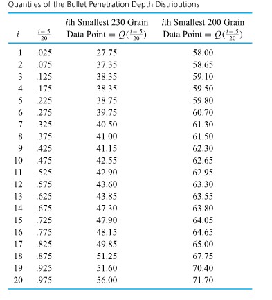
 quantiles for the two distributions of bullet penetration depth introduced in the previous section. For the 230 grain bullet penetration depths, interpolation yields
 & =.5 Q(.225)+.5 Q(.275)=.5(38.75)+.5(39.75)=39.25 \mathrm{~mm} \\Q(.5) & =.5 Q(.475)+.5 Q(.525)=.5(42.55)+.5(42.90)=42.725 \mathrm{~mm} \\Q(.75) & =.5 Q(.725)+.5 Q(.775)=.5(47.90)+.5(48.15)=48.025 \mathrm{~mm}\end{aligned}")
+1.5 I Q R & =61.188 \mathrm{~mm} \\Q(.25)-1.5 I Q R & =26.087 \mathrm{~mm}\end{aligned}")
 & =60.25 \mathrm{~mm} \\Q(.5) & =62.80 \mathrm{~mm} \\Q(.75) & =64.35 \mathrm{~mm} \\Q(.75)+1.5 I Q R & =70.50 \mathrm{~mm} \\Q(.25)-1.5 I Q R & =54.10 \mathrm{~mm}\end{aligned}")

 plot.
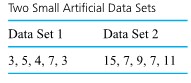
plot. th smallest value in data set 1
+1")
 and
and  stand for the quantile functions of the two respective data sets, it is clear from display (2.1.7.1) that
=2 Q_{1}(p)+1")
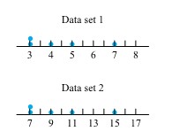

, \quad Q_{2}\left(\frac{i-.5}{5}\right)\right)")
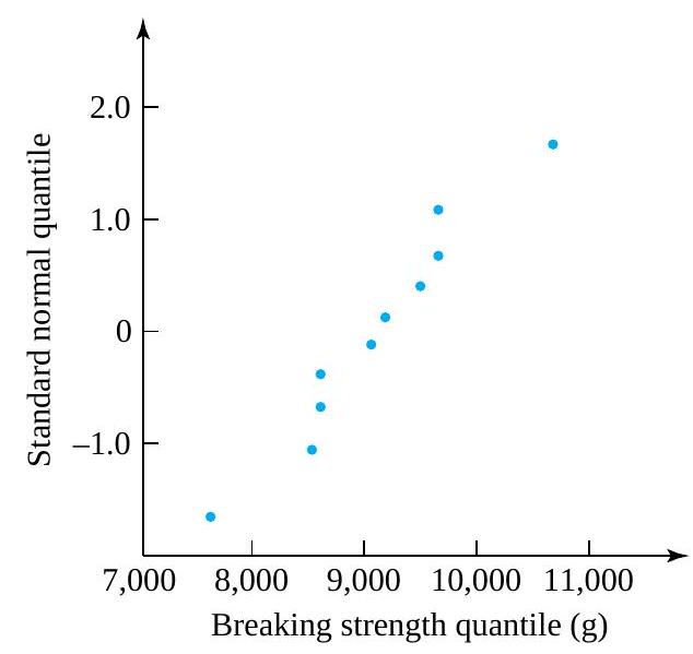
 ) should be exactly linear. Figure 3.16 illustrates this-in fact Figure 3.16 is a
 , Q_{2}(p)\right)") for appropriate values of
for appropriate values of  . When two data sets of unequal sizes are involved, the values of
  and
and  (for the 230 grain data) is out of proportion to the gap between 63.55 and
  (for the 200 grain data). This hints that there was some kind of basic physical difference in the mechanisms that produced the smaller and larger 230 grain penetration depths. Once this kind of indication is discovered, it is a task for ballistics experts or materials people to explain the phenomenon.
") , there is also a drastic difference in the shapes of the extreme lower ends of the two distributions. In order to move that point back on line with the rest of the plotted points, it would need to be moved to the right or down (i.e., increase the smallest 230 grain observation or decrease the smallest 200 grain observation). That is, relative to the 200 grain distribution, the 230 grain distribution is long-tailed to the low side. (Or to put it differently, relative to the 230 grain distribution, the 200 grain distribution is short-tailed to the low side.) Note that the difference in shapes was already evident in the boxplot in Figure previously. Again, it would remain for a specialist to explain this difference in distributional shapes.
, there is also a drastic difference in the shapes of the extreme lower ends of the two distributions. In order to move that point back on line with the rest of the plotted points, it would need to be moved to the right or down (i.e., increase the smallest 230 grain observation or decrease the smallest 200 grain observation). That is, relative to the 200 grain distribution, the 230 grain distribution is long-tailed to the low side. (Or to put it differently, relative to the 230 grain distribution, the 200 grain distribution is short-tailed to the low side.) Note that the difference in shapes was already evident in the boxplot in Figure previously. Again, it would remain for a specialist to explain this difference in distributional shapes.
\right)")
 , locate the entry in the row labelled by the first digit after the decimal place and in the column labelled by the second digit after the decimal place. (For example,
 =-.33") .) A simple numerical approximation to the values given in Table 3.10 adequate for most plotting purposes is
.) A simple numerical approximation to the values given in Table 3.10 adequate for most plotting purposes is \approx 4.9\left(p^{.14}-(1-p)^{.14}\right)")
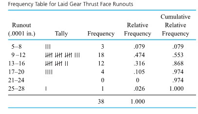
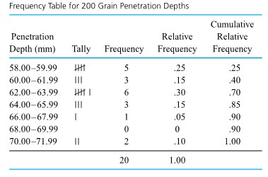
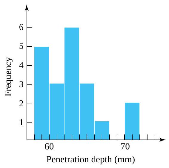
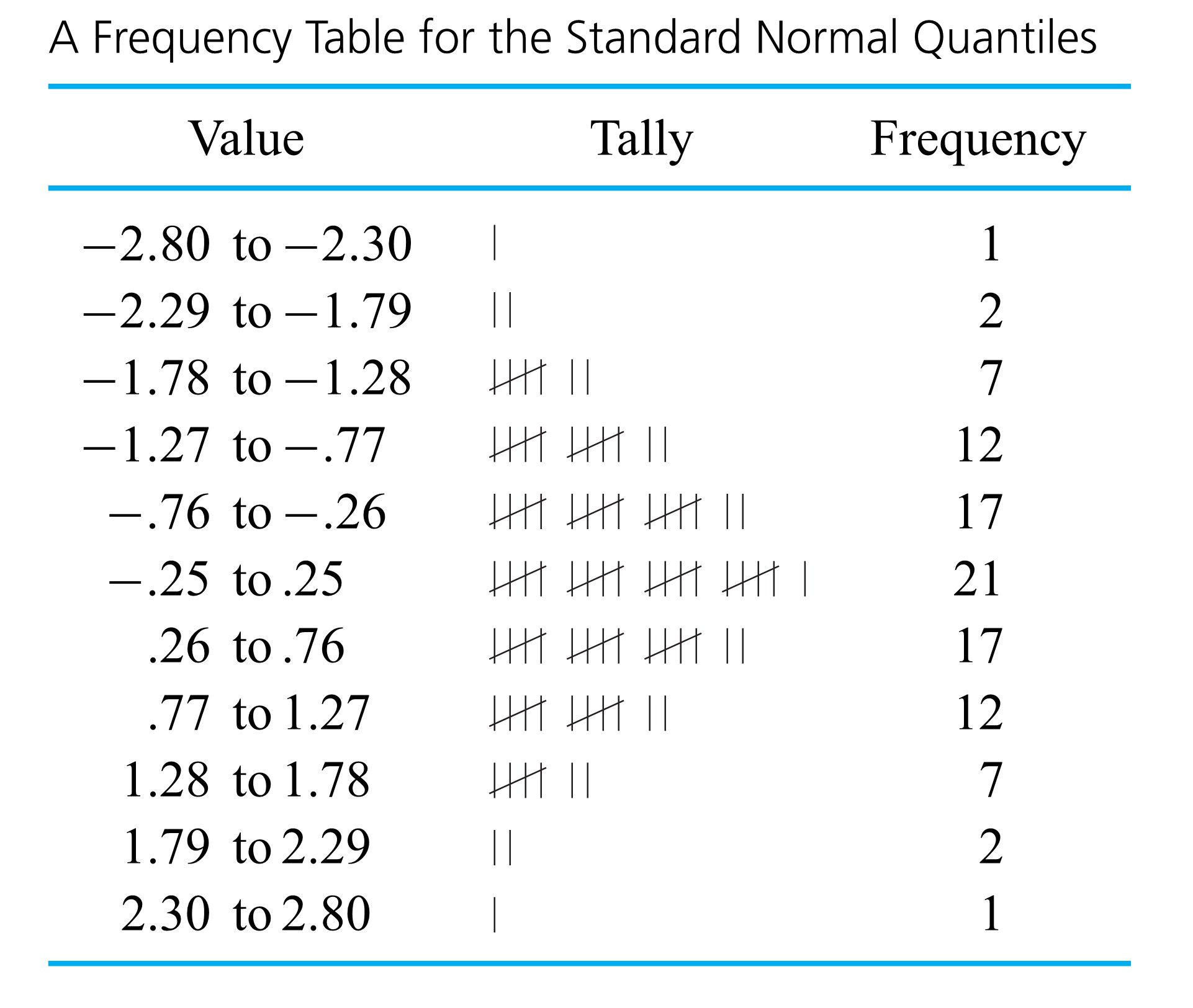
 . A possible frequency table for those 99 data points is given as Table 2.1.7.3. The tally column in Table 2.1.7.3 shows clearly the bell shape.
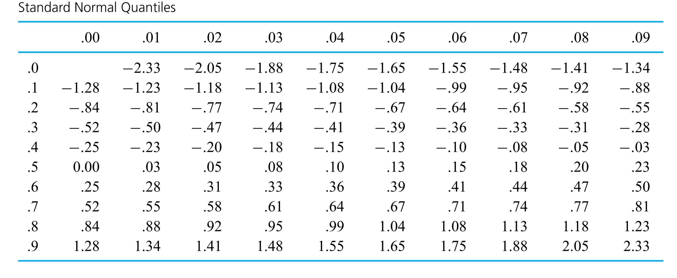
![Q-Q[l/atex] plotting here makes it possible to emphasize the relationship between probability plotting and (empirical) [latex]Q-Q](https://atu0g9ctah.execute-api.ca-central-1.amazonaws.com/latest/latex?latex=Q-Q%5Bl%2Fatex%5D%20plotting%20here%20makes%20it%20possible%20to%20emphasize%20the%20relationship%20between%20probability%20plotting%20and%20%28empirical%29%20%5Blatex%5DQ-Q&fg=000000&font=TeX&svg=1 "Q-Q[l/atex] plotting here makes it possible to emphasize the relationship between probability plotting and (empirical) [latex]Q-Q") plotting.
plotting.
 and/or the value 2 is replaced by
  .
. , is
, is
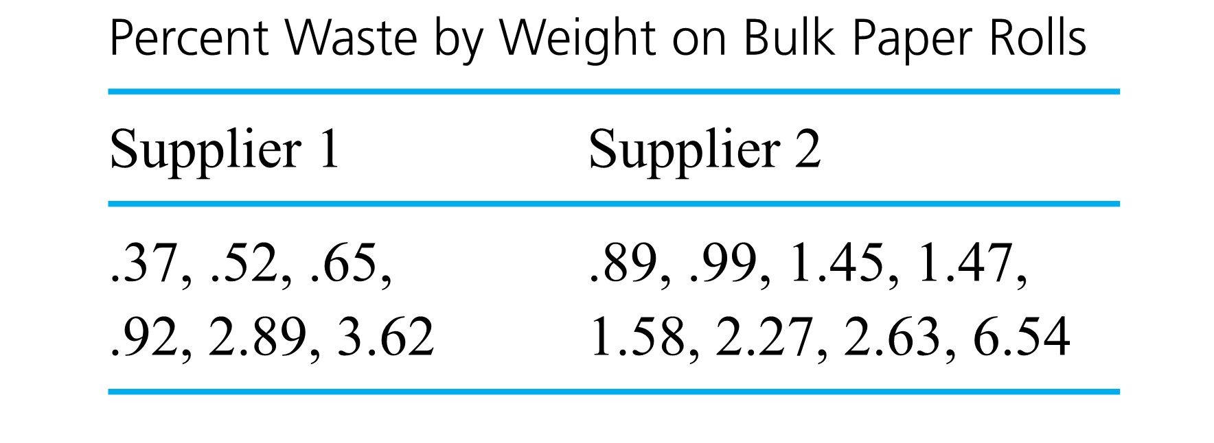
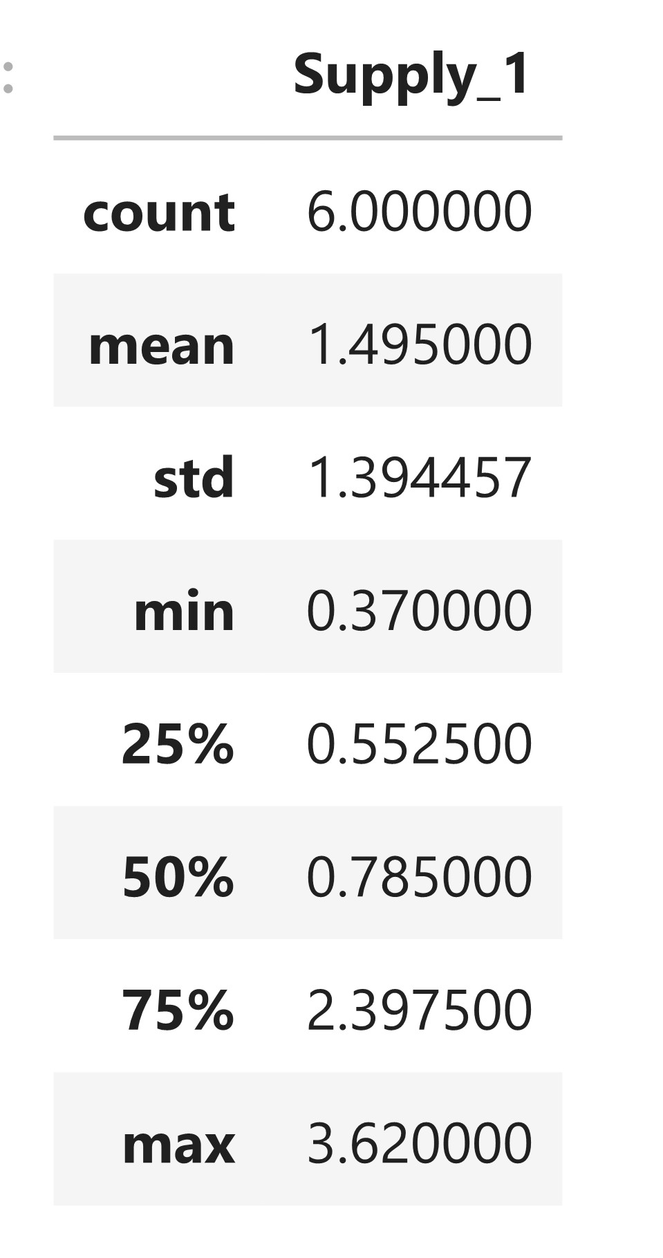
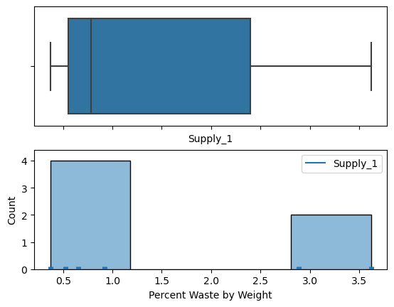
=.5(.65)+.5(.92)=.785 \% \text { waste }")
=1.495 \% \text { waste }")
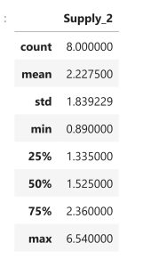
 \\ & =2.228 \% \text { waste }\end{aligned}")

 is
is
=18") .” Since the range depends only on the values of the smallest and largest points in a data set, it is necessarily highly sensitive to extreme (or outlying) values. Because it is easily calculated, it has enjoyed long-standing popularity in industrial settings, particularly as a tool in statistical quality control.
.” Since the range depends only on the values of the smallest and largest points in a data set, it is necessarily highly sensitive to extreme (or outlying) values. Because it is easily calculated, it has enjoyed long-standing popularity in industrial settings, particularly as a tool in statistical quality control. is
is^{2}")
 , is the nonnegative square root of the sample variance.
 for
for  is an average squared distance of the data points from the central value
 =.52 \\& Q(.75)=2.89\end{aligned}")


^{2}+(.52-1.495)^{2}+(.65-1.495)^{2}+(.92-1.495)^{2}\right. \\& \left.+(2.89-1.495)^{2}+(3.62-1.495)^{2}\right) \\= & 1.945(\% \text { waste })^{2}\end{aligned}")


^{2}+(.99-2.228)^{2}+(1.45-2.228)^{2}+(1.47-2.228)^{2}\right. \\& \left.+(1.58-2.228)^{2}+(2.27-2.228)^{2}+(2.63-2.228)^{2}+(6.54-2.228)^{2}\right) \\= & 3.383(\% \text { waste })^{2}\end{aligned}")

 and
and ") to stand for the population mean and to write:
to stand for the population mean and to write:
 is used in place of
 ") to stand for the population variance and to define:
to stand for the population variance and to define:^2")
 is then called the population standard deviation,
 different
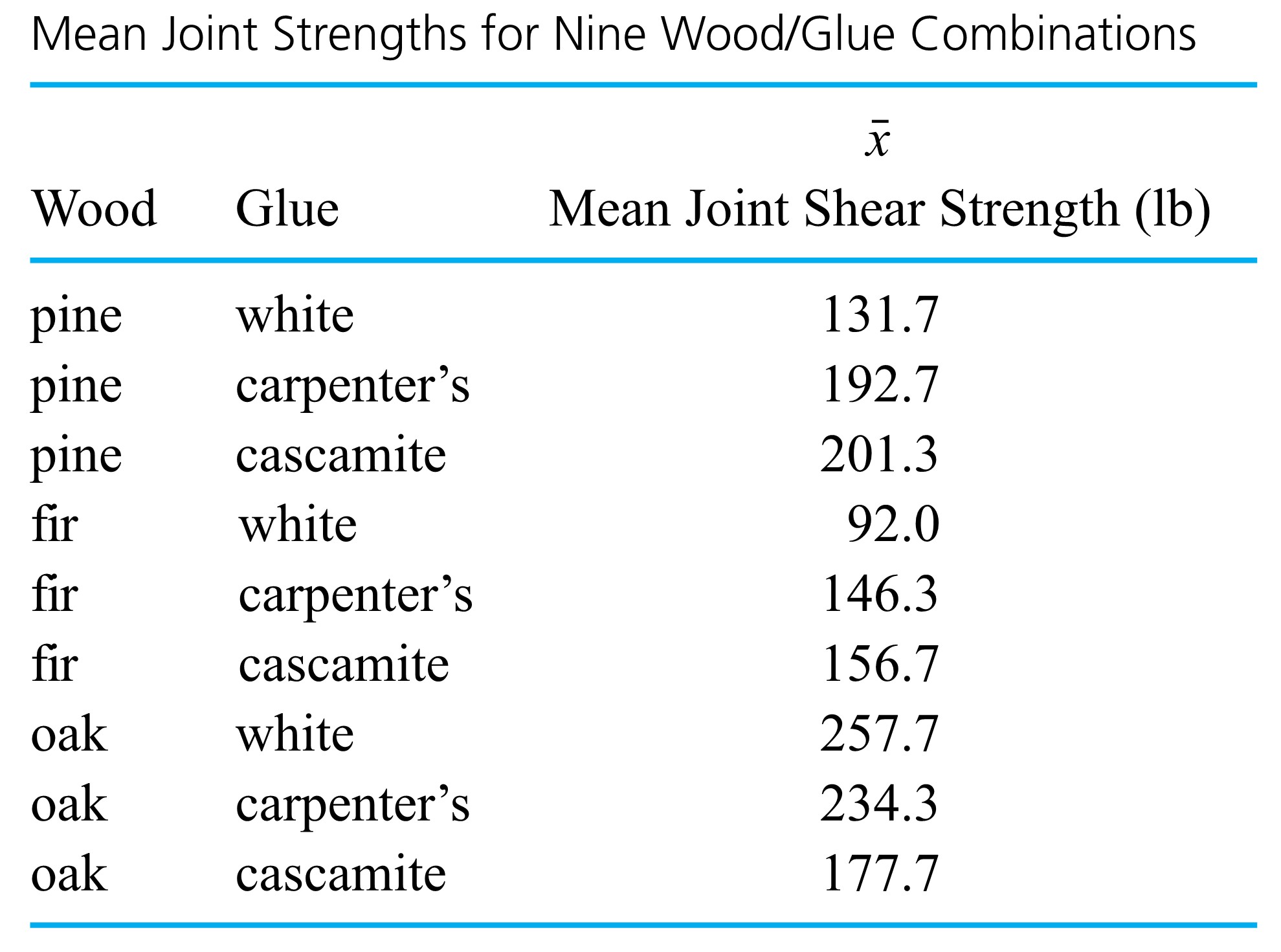
 or
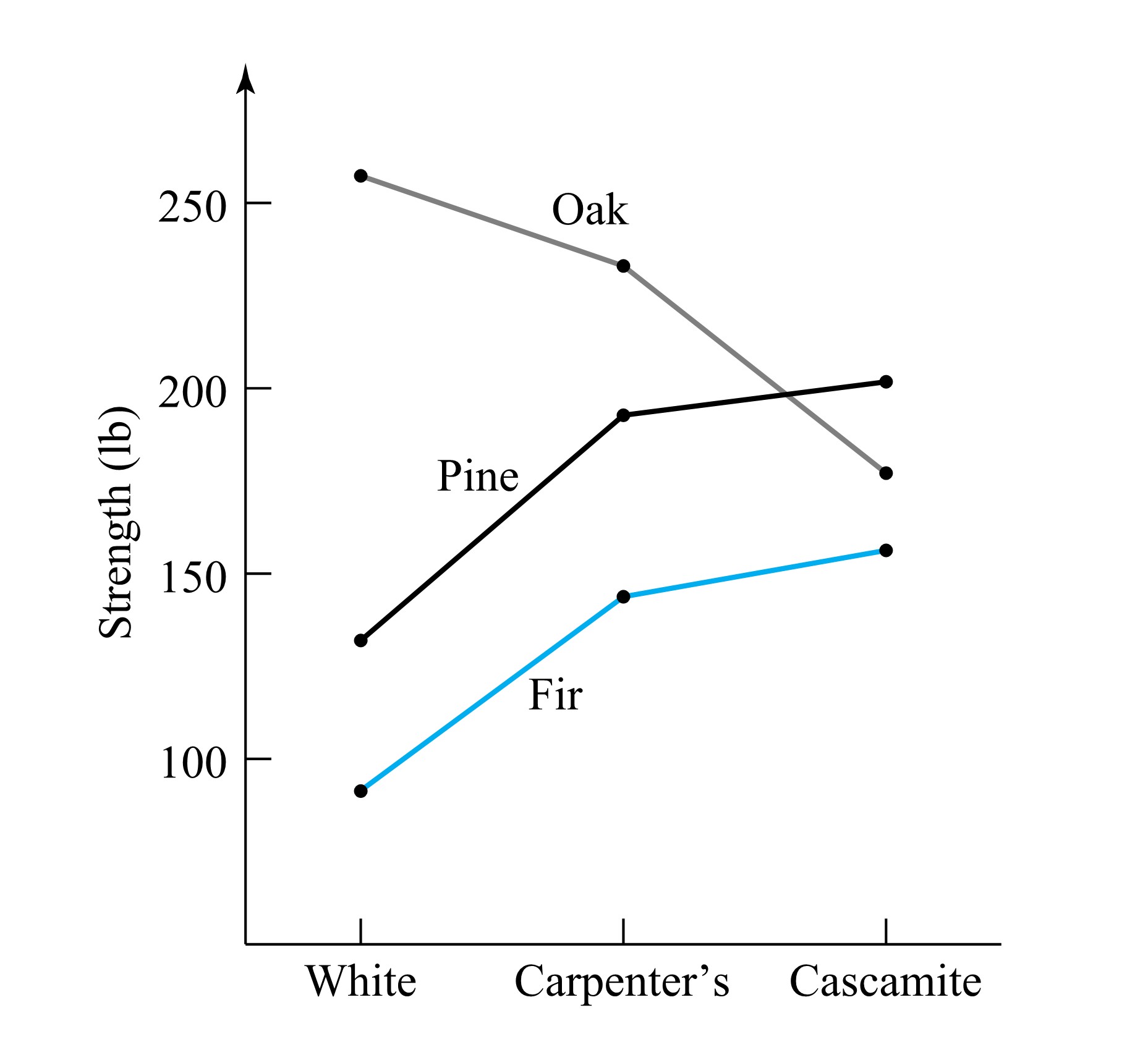
or  that need to be compared. Bar charts and simple bivariate plots can be a great aid in summarizing these results.
![30 \times 100=3,000[latex] connectors were inspected over this period,</div> <div> <div style="text-align: center">[latex]\begin{aligned}& \hat{p}_{\mathrm{A}}=3 / 3000=.0010 \\& \hat{p}_{\mathrm{B}}=0 / 3000=.0000 \\& \hat{p}_{\mathrm{C}}=11 / 3000=.0037 \\& \hat{p}_{\mathrm{D}}=1 / 3000=.0003\end{aligned}](https://atu0g9ctah.execute-api.ca-central-1.amazonaws.com/latest/latex?latex=30%20%5Ctimes%20100%3D3%2C000%5Blatex%5D%20connectors%20were%20inspected%20over%20this%20period%2C%3C%2Fdiv%3E%20%20%3Cdiv%3E%20%20%3Cdiv%20style%3D%22text-align%3A%20center%22%3E%5Blatex%5D%5Cbegin%7Baligned%7D%26%20%5Chat%7Bp%7D_%7B%5Cmathrm%7BA%7D%7D%3D3%20%2F%203000%3D.0010%20%5C%5C%26%20%5Chat%7Bp%7D_%7B%5Cmathrm%7BB%7D%7D%3D0%20%2F%203000%3D.0000%20%5C%5C%26%20%5Chat%7Bp%7D_%7B%5Cmathrm%7BC%7D%7D%3D11%20%2F%203000%3D.0037%20%5C%5C%26%20%5Chat%7Bp%7D_%7B%5Cmathrm%7BD%7D%7D%3D1%20%2F%203000%3D.0003%5Cend%7Baligned%7D&fg=000000&font=TeX&svg=1 "30 \times 100=3,000[latex] connectors were inspected over this period,</div> <div> <div style="text-align: center">[latex]\begin{aligned}& \hat{p}_{\mathrm{A}}=3 / 3000=.0010 \\& \hat{p}_{\mathrm{B}}=0 / 3000=.0000 \\& \hat{p}_{\mathrm{C}}=11 / 3000=.0037 \\& \hat{p}_{\mathrm{D}}=1 / 3000=.0003\end{aligned}")
") , because categories A through E represent a set of nonoverlapping and exhaustive classifications into which an individual connector must fall, so that the
, because categories A through E represent a set of nonoverlapping and exhaustive classifications into which an individual connector must fall, so that the 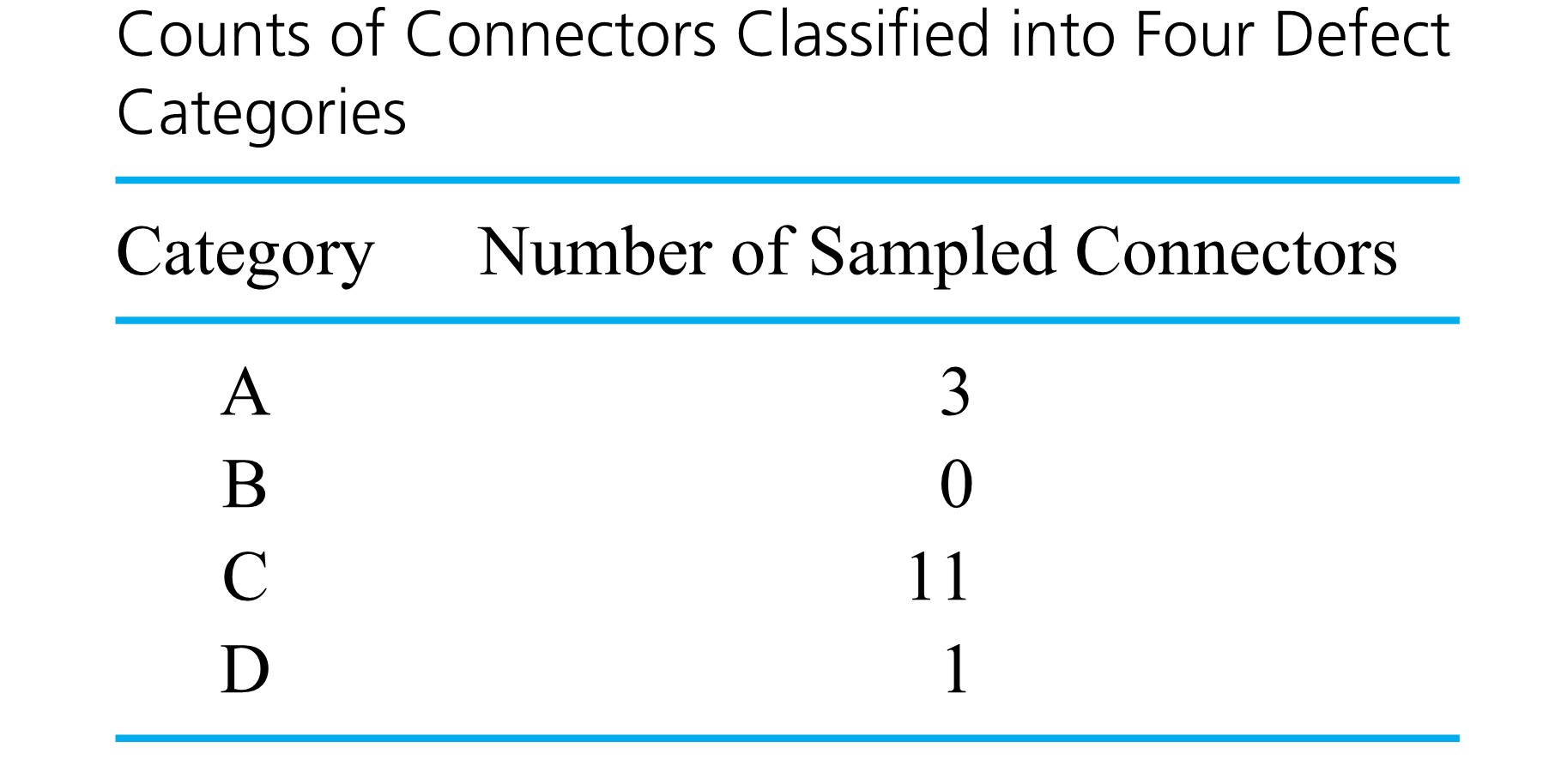
 , having moderately serious defects but no serious or very serious defects. This bar chart is a presentation of the behavior of a single categorical variable.
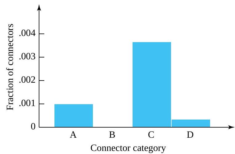

 , so
, so  for the fraction of tools without type 1 leaks. The
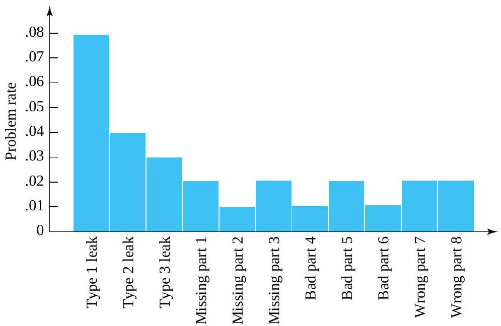
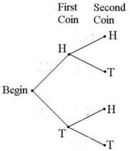
 where H = heads and T = tails are the outcomes. The sample space for flipping two fair coins once is shown: S = {(HH),(HT),(TH),(TT)}. We will also use capital letters to denote an event, like A and B. For example, we can define event A as realizing tails on the first coin and event B= tails on the second coin. This would be shown as
  and
and  . Using diagrams is helpful in representing the operations of multiple events together.
 is in neither
  nor
nor  . The Venn diagram is as follows:
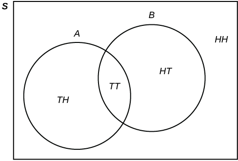
 . The marginal events are those shown on the margins of the table, and are those that occur for a single event with no regard for the other events in the table. For our example, we have marginal event A and the associated joint events,
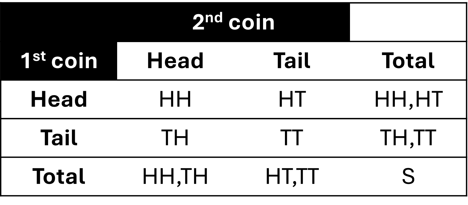
 .
. .
. .
. .
. is the set of outcomes that are in both
  is the set of outcomes that are in either
  . Therefore
  is the set of outcomes that are not in
  , with m being the number of outcomes in the the event A occurs and n being the total number of outcomes of the experiment. A claim of the frequentist approach is that, as the number of trials increases, the change in the relative frequency will diminish. Hence, one can view a probability as the limiting value of the corresponding relative frequencies. You can realize the relative frequency by either running real experiments and finding an empirical or estimated probability or by recognizing the theoretical model for the experiment and adopting a theoretical probability based on events from the sample space.
 = 0.5.
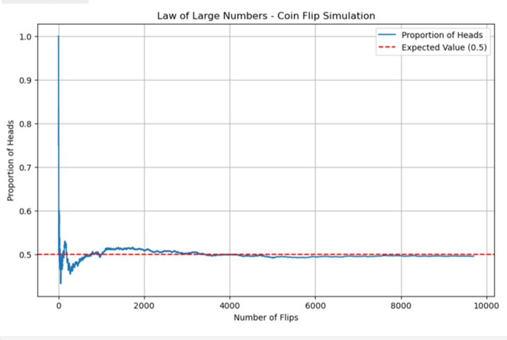
") , is assigned a number between zero and one, inclusive, and describes the proportion of time we expect the event to occur over the long-term. P(A) = 0 means the event A can never happen. P(A) = 1 means the event A always happens. P(A) = 0.5 means the event A is equally likely to occur or not to occur. For example, if you flip one fair coin repeatedly (from 20 to 2,000 to 20,000 times) the relative frequency of heads approaches 0.5 (the probability of heads).
, is assigned a number between zero and one, inclusive, and describes the proportion of time we expect the event to occur over the long-term. P(A) = 0 means the event A can never happen. P(A) = 1 means the event A always happens. P(A) = 0.5 means the event A is equally likely to occur or not to occur. For example, if you flip one fair coin repeatedly (from 20 to 2,000 to 20,000 times) the relative frequency of heads approaches 0.5 (the probability of heads). is 1 and the probability of the empty set is 0. This is: P(S) = 1 and P(∅) = 0.
 = \sum_{n= 1}^\infty P(A_n)")
 = \frac{P(A \cap B)}{P(B)}")
") as “the probability of A given B”.
as “the probability of A given B”. = P(A)P(B)") .
. = P(A)") .
. = P(B)") .
. are mutually independent if for any sub-collection
  there is:
 = P(A_{i_1}) \cdot P(A_{i_2}) \cdot \ldots \cdot P(A_{i_k})")
 cards. It consists of four suits. The suits are clubs, diamonds, hearts and spades. There are
  cards in each suit consisting of
  ,
,  (jack),
  (queen),
  (king) of that suit.
 cards remaining in the deck. It is the three of diamonds. You put this card aside and pick the third card from the remaining
  cards in the deck. The third card is the

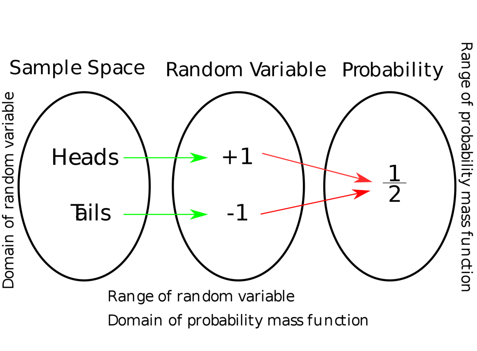
![{\displaystyle [0,1]\subseteq \mathbb {R} }](https://atu0g9ctah.execute-api.ca-central-1.amazonaws.com/latest/latex?latex=%7B%5Cdisplaystyle%20%5B0%2C1%5D%5Csubseteq%20%5Cmathbb%20%7BR%7D%20%7D&fg=000000&font=TeX&svg=1 "{\displaystyle [0,1]\subseteq \mathbb {R} }") , which provides the probability measure on the set of all possible values of the random variable. Random variables are shown as Roman capital letters, often towards the end of the alphabet, such as
, which provides the probability measure on the set of all possible values of the random variable. Random variables are shown as Roman capital letters, often towards the end of the alphabet, such as  .
. to a measurable space of
  , where 1 is correspondent to H and -1 is correspondent to T, utilizing a random variable of
  =
=  = +1, written as
 ") .
.
") for an event.
for an event.") .
.![{\displaystyle F\colon \mathbb {R} \rightarrow [0,1]}](https://atu0g9ctah.execute-api.ca-central-1.amazonaws.com/latest/latex?latex=%7B%5Cdisplaystyle%20F%5Ccolon%20%5Cmathbb%20%7BR%7D%20%5Crightarrow%20%5B0%2C1%5D%7D&fg=000000&font=TeX&svg=1 "{\displaystyle F\colon \mathbb {R} \rightarrow [0,1]}") , where
, where =0}") and
and =1}") . Every function with these four properties is a CDF: for every such function, a random variable can be defined such that the function is the cumulative distribution function of that random variable.
. Every function with these four properties is a CDF: for every such function, a random variable can be defined such that the function is the cumulative distribution function of that random variable.![F(x)=P[X \leq x]](https://atu0g9ctah.execute-api.ca-central-1.amazonaws.com/latest/latex?latex=F%28x%29%3DP%5BX%20%5Cleq%20x%5D&fg=000000&font=TeX&svg=1 "F(x)=P[X \leq x]")
 ,
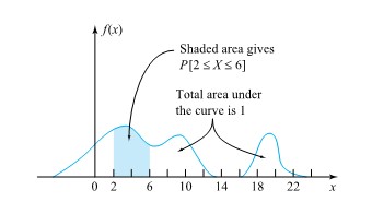
, ,…, is a non-negative function f (x ), with f (
 ) giving the probability that X takes the value
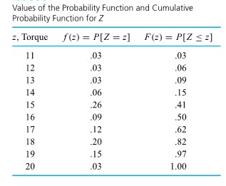
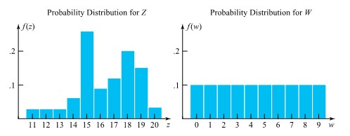
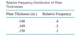
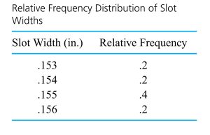
 = the next measured torque for bolt 3 (recorded to the nearest integer), and we will treat Z as a discrete random variable. Now we want to give a plausible probility function for it. The relative frequencies for the bolt 3 torque measurements recorded introduce the relative frequency distribution:
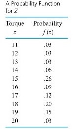
 = the torque value selected.
= \begin{cases}.1 & \text { for } w=0,1,2, \ldots, 9 \\ 0 & \text { otherwise }\end{cases}")
![F(16.3)=P[Z \leq 16.3]=P[Z \leq 16]=F(16)=.50](https://atu0g9ctah.execute-api.ca-central-1.amazonaws.com/latest/latex?latex=F%2816.3%29%3DP%5BZ%20%5Cleq%2016.3%5D%3DP%5BZ%20%5Cleq%2016%5D%3DF%2816%29%3D.50&fg=000000&font=TeX&svg=1 "F(16.3)=P[Z \leq 16.3]=P[Z \leq 16]=F(16)=.50")
![F(32)=P[Z \leq 32]=1.00](https://atu0g9ctah.execute-api.ca-central-1.amazonaws.com/latest/latex?latex=F%2832%29%3DP%5BZ%20%5Cleq%2032%5D%3D1.00&fg=000000&font=TeX&svg=1 "F(32)=P[Z \leq 32]=1.00")

")
")
^2 f(x) \quad\left(=\sum x^2 f(x)-(E X)^2\right)")
 . Often the notation
  is used in place of Var X, and
  = 2.15 ft lb
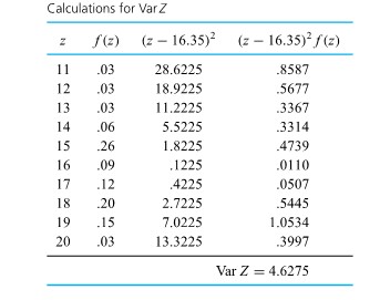
") .
.
-(E W)^2=28.5-(4.5)^2=8.25")


![X[latex] has the <strong>binomial (n, p) distribution</strong>.</div> <div> <div> <div class="textbox"> <strong>DEFINITION 3.2.5.1. Binomial Definition</strong> The binomial [latex](n, p)](https://atu0g9ctah.execute-api.ca-central-1.amazonaws.com/latest/latex?latex=X%5Blatex%5D%20has%20the%20%3Cstrong%3Ebinomial%20%28n%2C%20p%29%20distribution%3C%2Fstrong%3E.%3C%2Fdiv%3E%20%20%3Cdiv%3E%20%20%3Cdiv%3E%20%20%3Cdiv%20class%3D%22textbox%22%3E%20%20%20%20%3Cstrong%3EDEFINITION%203.2.5.1.%20Binomial%20Definition%3C%2Fstrong%3E%20%20%20%20The%20binomial%20%5Blatex%5D%28n%2C%20p%29&fg=000000&font=TeX&svg=1 "X[latex] has the <strong>binomial (n, p) distribution</strong>.</div> <div> <div> <div class="textbox"> <strong>DEFINITION 3.2.5.1. Binomial Definition</strong> The binomial [latex](n, p)") distribution is a discrete probability distribution with probability function
distribution is a discrete probability distribution with probability function = \begin{cases}\frac{n !}{x !(n-x) !} p^{x}(1-p)^{n-x} & \text { for } x=0,1, \ldots, n \\ 0 & \text { otherwise }\end{cases}")
 .
.") for each trial producing a no go/failure outcome. And the
for each trial producing a no go/failure outcome. And the  !") term is a count of the number of patterns in which it would be possible to see
term is a count of the number of patterns in which it would be possible to see  nomial distribution derives from the fact that the values
 , f(1), f(2), \ldots, f(n)") are the terms in the expansion of
are the terms in the expansion of)^{n}")
 , the resulting histogram is right-skewed. For
  , the resulting histogram is left-skewed. The skewness increases as
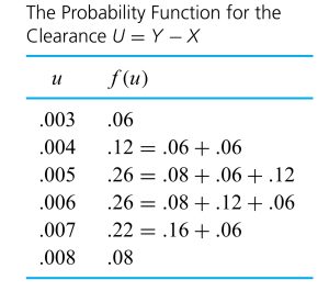
 is indeed a sensible figure for the chance that a given shaft will be reworkable. Suppose further that
![\begin{aligned}P[\text { at least two reworkable shafts] } & =P[U \geq 2] \\& =f(2)+f(3)+\cdots+f(10) \\& =1-(f(0)+f(1)) \\& =1-\left(\frac{10 !}{0 ! 10 !}(.2)^{0}(.8)^{10}+\frac{10 !}{1 ! 9 !}(.2)^{1}(.8)^{9}\right) \\&=.62\end{aligned}](https://atu0g9ctah.execute-api.ca-central-1.amazonaws.com/latest/latex?latex=%5Cbegin%7Baligned%7DP%5B%5Ctext%20%7B%20at%20least%20two%20reworkable%20shafts%5D%20%7D%20%26%20%3DP%5BU%20%5Cgeq%202%5D%20%5C%5C%26%20%3Df%282%29%2Bf%283%29%2B%5Ccdots%2Bf%2810%29%20%5C%5C%26%20%3D1-%28f%280%29%2Bf%281%29%29%20%5C%5C%26%20%3D1-%5Cleft%28%5Cfrac%7B10%20%21%7D%7B0%20%21%2010%20%21%7D%28.2%29%5E%7B0%7D%28.8%29%5E%7B10%7D%2B%5Cfrac%7B10%20%21%7D%7B1%20%21%209%20%21%7D%28.2%29%5E%7B1%7D%28.8%29%5E%7B9%7D%5Cright%29%20%5C%5C%26%3D.62%5Cend%7Baligned%7D&fg=000000&font=TeX&svg=1 "\begin{aligned}P[\text { at least two reworkable shafts] } & =P[U \geq 2] \\& =f(2)+f(3)+\cdots+f(10) \\& =1-(f(0)+f(1)) \\& =1-\left(\frac{10 !}{0 ! 10 !}(.2)^{0}(.8)^{10}+\frac{10 !}{1 ! 9 !}(.2)^{1}(.8)^{9}\right) \\&=.62\end{aligned}")
") 's have to sum up to 1 , is a common and useful one.)
's have to sum up to 1 , is a common and useful one.) , and the . 62 figure largely irrelevant. (The independence-of-trials assumption would be inappropriate in this situation.)
") .
. from it.
 is obtained as follows. Possible values for
 ![\begin{aligned}f(0)= & P[V=0] \\= & P[\text { first pellet selected is nonconforming and } \\& \text { subsequently the second pellet is also nonconforming }] \\f(2)= & P[V=2] \\= & P[\text { first pellet selected is conforming and } \\& \text { subsequently the second pellet selected is conforming }] \\f(1)= & 1-(f(0)+f(2))\end{aligned}](https://atu0g9ctah.execute-api.ca-central-1.amazonaws.com/latest/latex?latex=%5Cbegin%7Baligned%7Df%280%29%3D%20%26%20P%5BV%3D0%5D%20%5C%5C%3D%20%26%20P%5B%5Ctext%20%7B%20first%20pellet%20selected%20is%20nonconforming%20and%20%7D%20%5C%5C%26%20%5Ctext%20%7B%20subsequently%20the%20second%20pellet%20is%20also%20nonconforming%20%7D%5D%20%5C%5Cf%282%29%3D%20%26%20P%5BV%3D2%5D%20%5C%5C%3D%20%26%20P%5B%5Ctext%20%7B%20first%20pellet%20selected%20is%20conforming%20and%20%7D%20%5C%5C%26%20%5Ctext%20%7B%20subsequently%20the%20second%20pellet%20selected%20is%20conforming%20%7D%5D%20%5C%5Cf%281%29%3D%20%26%201-%28f%280%29%2Bf%282%29%29%5Cend%7Baligned%7D&fg=000000&font=TeX&svg=1 "\begin{aligned}f(0)= & P[V=0] \\= & P[\text { first pellet selected is nonconforming and } \\& \text { subsequently the second pellet is also nonconforming }] \\f(2)= & P[V=2] \\= & P[\text { first pellet selected is conforming and } \\& \text { subsequently the second pellet selected is conforming }] \\f(1)= & 1-(f(0)+f(2))\end{aligned}")
") is
is=\frac{34}{100} \cdot \frac{33}{99}=.1133")
=\frac{66}{100} \cdot \frac{65}{99}=.4333")
=1-(.1133+.4333)=1-.5467=.4533")
 to
to  . Nevertheless, for most practical purposes,
  . To see this, note that
^{2}(.66)^{0}=.1156 \approx f(0) \\& \frac{2 !}{1 ! 1 !}(.34)^{1}(.66)^{1}=.4488 \approx f(1) \\& \frac{2 !}{2 ! 0 !}(.34)^{0}(.66)^{2}=.4356 \approx f(2)\end{aligned}")
 is not too extreme, and a binomial distribution is a decent description of a variable arising from simple random sampling.
 !} p^{x}(1-p)^{n-x}=n p")
^{2} \frac{n !}{x !(n-x) !} p^{x}(1-p)^{n-x}=n p(1-p)")
(.2)=2 \text { shafts } \\\sqrt{\operatorname{Var} U} & =\sqrt{10(.2)(.8)}=1.26 \text { shafts }\end{aligned}")
") distribution
distribution= \begin{cases}\frac{e^{-\lambda} \lambda^{x}}{x !} & \text { for } x=0,1,2, \ldots \\ 0 & \text { otherwise }\end{cases}")
 .
. . One is then led to the binomial
  ) distribution. In fact, for large
 ") probability function approximates the one specified in equation (5.10). So one might think of the Poisson distribution for counts as arising through a mechanism that would present many tiny similar opportunities for independent occurrence or non-occurrence throughout an interval of time or space.
probability function approximates the one specified in equation (5.10). So one might think of the Poisson distribution for counts as arising through a mechanism that would present many tiny similar opportunities for independent occurrence or non-occurrence throughout an interval of time or space.
 , whose probability histograms peak near their respective
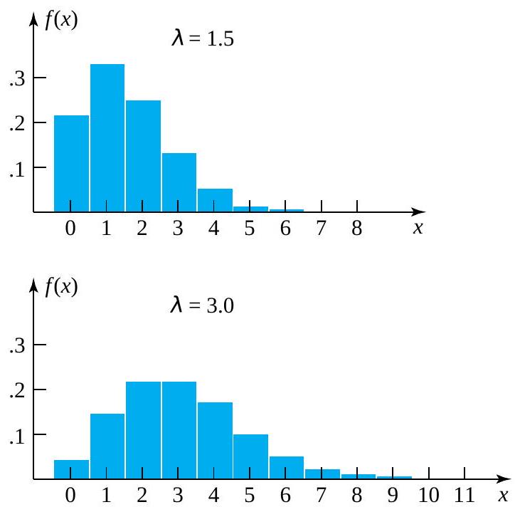

^{2} \frac{e^{-\lambda} \lambda^{x}}{x !}=\lambda")
 -Particles
 .
.
= \begin{cases}\frac{e^{-3.87}(3.87)^{s}}{s !} & \text { for } s=0,1,2, \ldots \\ 0 & \text { otherwise }\end{cases}")
 [at least 4 particles are recorded]
![=P[S \geq 4]](https://atu0g9ctah.execute-api.ca-central-1.amazonaws.com/latest/latex?latex=%3DP%5BS%20%5Cgeq%204%5D&fg=000000&font=TeX&svg=1 "=P[S \geq 4]")
+f(5)+f(6)+\cdots")
+f(1)+f(2)+f(3))")
^{0}}{0 !}+\frac{e^{-3.87}(3.87)^{1}}{1 !}+\frac{e^{-3.87}(3.87)^{2}}{2 !}+\frac{e^{-3.87}(3.87)^{3}}{3 !}\right)")


 , the reasonable choice of
 =12.5 \text { students }")

![\begin{aligned}P[10 \leq M \leq 15]= & f(10)+f(11)+f(12)+f(13)+f(14)+f(15) \\= & \frac{e^{-12.5}(12.5)^{10}}{10 !}+\frac{e^{-12.5}(12.5)^{11}}{11 !}+\frac{e^{-12.5}(12.5)^{12}}{12 !} \\& +\frac{e^{-12.5}(12.5)^{13}}{13 !}+\frac{e^{-12.5}(12.5)^{14}}{14 !}+\frac{e^{-12.5}(12.5)^{15}}{15 !} \\= & .60\end{aligned}](https://atu0g9ctah.execute-api.ca-central-1.amazonaws.com/latest/latex?latex=%5Cbegin%7Baligned%7DP%5B10%20%5Cleq%20M%20%5Cleq%2015%5D%3D%20%26%20f%2810%29%2Bf%2811%29%2Bf%2812%29%2Bf%2813%29%2Bf%2814%29%2Bf%2815%29%20%5C%5C%3D%20%26%20%5Cfrac%7Be%5E%7B-12.5%7D%2812.5%29%5E%7B10%7D%7D%7B10%20%21%7D%2B%5Cfrac%7Be%5E%7B-12.5%7D%2812.5%29%5E%7B11%7D%7D%7B11%20%21%7D%2B%5Cfrac%7Be%5E%7B-12.5%7D%2812.5%29%5E%7B12%7D%7D%7B12%20%21%7D%20%5C%5C%26%20%2B%5Cfrac%7Be%5E%7B-12.5%7D%2812.5%29%5E%7B13%7D%7D%7B13%20%21%7D%2B%5Cfrac%7Be%5E%7B-12.5%7D%2812.5%29%5E%7B14%7D%7D%7B14%20%21%7D%2B%5Cfrac%7Be%5E%7B-12.5%7D%2812.5%29%5E%7B15%7D%7D%7B15%20%21%7D%20%5C%5C%3D%20%26%20.60%5Cend%7Baligned%7D&fg=000000&font=TeX&svg=1 "\begin{aligned}P[10 \leq M \leq 15]= & f(10)+f(11)+f(12)+f(13)+f(14)+f(15) \\= & \frac{e^{-12.5}(12.5)^{10}}{10 !}+\frac{e^{-12.5}(12.5)^{11}}{11 !}+\frac{e^{-12.5}(12.5)^{12}}{12 !} \\& +\frac{e^{-12.5}(12.5)^{13}}{13 !}+\frac{e^{-12.5}(12.5)^{14}}{14 !}+\frac{e^{-12.5}(12.5)^{15}}{15 !} \\= & .60\end{aligned}")

 dx") = 1
= 1 dx")
") to represent the curve.
to represent the curve.  f (x ) dx values as dx gets small. (In mechanics,
  X
X f(t) dt
 F(x) = f(x)
 and
and  . P(c<x<d) is the area under the curve, above the x-axis, to the right of
 =0") . The probability that
. The probability that  and
and  ). Since the probability is equal to the area, the probability is also zero.
") because probability is equal to area.
because probability is equal to area. d x") .
.^2 f(x) d x \quad\left(=\int_{-\infty}^{\infty} x^2 f(x) d x-(E X)^2\right)")
 is used in place of Var X ,and σ is used in place of
 =\frac{1}{\sqrt{2 \pi \sigma^2}} e^{-(x-\mu)^2 / 2 \sigma^2}")
^2 / 2 \sigma^2} d x=\mu")
^2 \frac{1}{\sqrt{2 \pi \sigma^2}} e^{-(x-\mu)^2 / 2 \sigma^2} d x=\sigma^2")
 (remember that the standard deviation =
  = σ). Figure 4.1.3.1 shows the notation for the standard normal distribution, and that the distribution shape depends on these parameters. Since the area under the curve must equal one, a change in the standard deviation, σ, causes a change in the shape of the curve; the curve becomes fatter or skinnier depending on σ. A change in μ causes the graph to shift to the left or right. This means there are an infinite number of normal probability distributions.

![P[a \leq X \leq b]=\int_a^b \frac{1}{\sqrt{2 \pi \sigma^2}} e^{-(x-\mu)^2 / 2 \sigma^2} d x=\int_{(a-\mu) / \sigma}^{(b-\mu) / \sigma} \frac{1}{\sqrt{2 \pi}} e^{-z^2 / 2} d z](https://atu0g9ctah.execute-api.ca-central-1.amazonaws.com/latest/latex?latex=P%5Ba%20%5Cleq%20X%20%5Cleq%20b%5D%3D%5Cint_a%5Eb%20%5Cfrac%7B1%7D%7B%5Csqrt%7B2%20%5Cpi%20%5Csigma%5E2%7D%7D%20e%5E%7B-%28x-%5Cmu%29%5E2%20%2F%202%20%5Csigma%5E2%7D%20d%20x%3D%5Cint_%7B%28a-%5Cmu%29%20%2F%20%5Csigma%7D%5E%7B%28b-%5Cmu%29%20%2F%20%5Csigma%7D%20%5Cfrac%7B1%7D%7B%5Csqrt%7B2%20%5Cpi%7D%7D%20e%5E%7B-z%5E2%20%2F%202%7D%20d%20z&fg=000000&font=TeX&svg=1 "P[a \leq X \leq b]=\int_a^b \frac{1}{\sqrt{2 \pi \sigma^2}} e^{-(x-\mu)^2 / 2 \sigma^2} d x=\int_{(a-\mu) / \sigma}^{(b-\mu) / \sigma} \frac{1}{\sqrt{2 \pi}} e^{-z^2 / 2} d z")

 / \sigma}^{(b-\mu) / \sigma} \frac{1}{\sqrt{2 \pi}} e^{-z^2 / 2} d z")
") and a value x associated with X , one converts to units of standard deviations above the mean via:
and a value x associated with X , one converts to units of standard deviations above the mean via: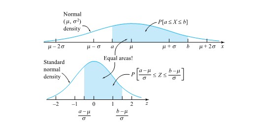
=F(z)=\int_{-\infty}^z \frac{1}{\sqrt{2 \pi}} e^{-t^2 / 2} d t")
") is used to stand for the standard normal cumulative probability function, instead of the more generic F.
is used to stand for the standard normal cumulative probability function, instead of the more generic F.") , the standard normal quantile function,
, the standard normal quantile function,\right) & =p \\ Q_z(\Phi(z)) & =z \end{array}\right\}")
 is not just a standard normal phenomenon but is true in general
=0.96")
-\Phi(0.57)")
 = .025 in the right tail of the standard normal
=.975") = .975. Locating .975 in the table body, one sees that z = 1.96.
= .975. Locating .975 in the table body, one sees that z = 1.96.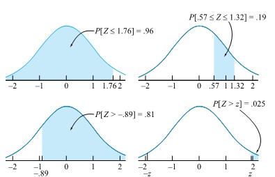

=.08")
 = 134.0 and w
 = 136.0 are converted to z-values (or units of standard deviations above the mean) as

-\Phi(-2.00)=.2266-.0228=.20")

=-2.33")


") , giving the probability that (simultaneously)
, giving the probability that (simultaneously)  . That is,
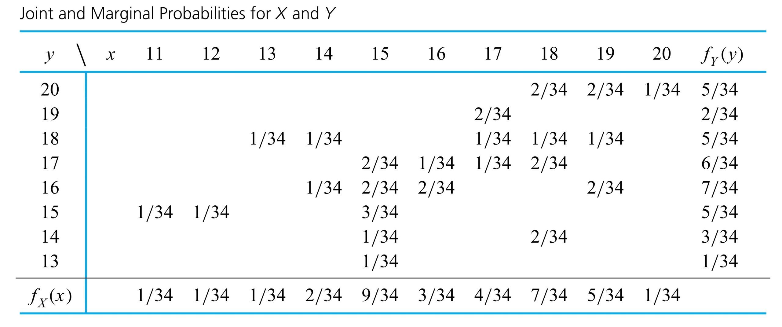
![f(x, y)=P[X=x \text { and } Y=y]](https://atu0g9ctah.execute-api.ca-central-1.amazonaws.com/latest/latex?latex=f%28x%2C%20y%29%3DP%5BX%3Dx%20%5Ctext%20%7B%20and%20%7D%20Y%3Dy%5D&fg=000000&font=TeX&svg=1 "f(x, y)=P[X=x \text { and } Y=y]")
 the next torque recorded for bolt 3
 the next torque recorded for bolt 4
 and
and ![Y=18]](https://atu0g9ctah.execute-api.ca-central-1.amazonaws.com/latest/latex?latex=Y%3D18%5D&fg=000000&font=TeX&svg=1 "Y=18]") might be
might be  , the relative frequency of this pair in the data set. Similarly, the assignments
![\begin{aligned}& P[X=18 \text { and } Y=17]=\frac{2}{34} \\& P[X=14 \text { and } Y=9]=0\end{aligned}](https://atu0g9ctah.execute-api.ca-central-1.amazonaws.com/latest/latex?latex=%5Cbegin%7Baligned%7D%26%20P%5BX%3D18%20%5Ctext%20%7B%20and%20%7D%20Y%3D17%5D%3D%5Cfrac%7B2%7D%7B34%7D%20%5C%5C%26%20P%5BX%3D14%20%5Ctext%20%7B%20and%20%7D%20Y%3D9%5D%3D0%5Cend%7Baligned%7D&fg=000000&font=TeX&svg=1 "\begin{aligned}& P[X=18 \text { and } Y=17]=\frac{2}{34} \\& P[X=14 \text { and } Y=9]=0\end{aligned}")

![[0,1]](https://atu0g9ctah.execute-api.ca-central-1.amazonaws.com/latest/latex?latex=%5B0%2C1%5D&fg=000000&font=TeX&svg=1 "[0,1]") and that they total to 1 . By summing up just some of the
and that they total to 1 . By summing up just some of the ![\begin{aligned}& P[X\geq Y], \\& P[|X-Y|\leq 1], \\& \text { and } P[X=17]\end{aligned}](https://atu0g9ctah.execute-api.ca-central-1.amazonaws.com/latest/latex?latex=%5Cbegin%7Baligned%7D%26%20P%5BX%5Cgeq%20Y%5D%2C%20%5C%5C%26%20P%5B%7CX-Y%7C%5Cleq%201%5D%2C%20%5C%5C%26%20%5Ctext%20%7B%20and%20%7D%20P%5BX%3D17%5D%5Cend%7Baligned%7D&fg=000000&font=TeX&svg=1 "\begin{aligned}& P[X\geq Y], \\& P[|X-Y|\leq 1], \\& \text { and } P[X=17]\end{aligned}")
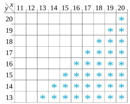
![P[X \geq Y]](https://atu0g9ctah.execute-api.ca-central-1.amazonaws.com/latest/latex?latex=P%5BX%20%5Cgeq%20Y%5D&fg=000000&font=TeX&svg=1 "P[X \geq Y]") , the probability that the measured bolt 3 torque is at least as big as the measured bolt 4 torque. Figure 4.2.1.1 indicates with asterisks which possible combinations of
, the probability that the measured bolt 3 torque is at least as big as the measured bolt 4 torque. Figure 4.2.1.1 indicates with asterisks which possible combinations of ![\begin{aligned}P[X \geq Y]= & f(15,13)+f(15,14)+f(15,15)+f(16,16) \\& +f(17,17)+f(18,14)+f(18,17)+f(18,18) \\& +f(19,16)+f(19,18)+f(20,20) \\= & \frac{1}{34}+\frac{1}{34}+\frac{3}{34}+\frac{2}{34}+\cdots+\frac{1}{34}=\frac{17}{34}\end{aligned}](https://atu0g9ctah.execute-api.ca-central-1.amazonaws.com/latest/latex?latex=%5Cbegin%7Baligned%7DP%5BX%20%5Cgeq%20Y%5D%3D%20%26%20f%2815%2C13%29%2Bf%2815%2C14%29%2Bf%2815%2C15%29%2Bf%2816%2C16%29%20%5C%5C%26%20%2Bf%2817%2C17%29%2Bf%2818%2C14%29%2Bf%2818%2C17%29%2Bf%2818%2C18%29%20%5C%5C%26%20%2Bf%2819%2C16%29%2Bf%2819%2C18%29%2Bf%2820%2C20%29%20%5C%5C%3D%20%26%20%5Cfrac%7B1%7D%7B34%7D%2B%5Cfrac%7B1%7D%7B34%7D%2B%5Cfrac%7B3%7D%7B34%7D%2B%5Cfrac%7B2%7D%7B34%7D%2B%5Ccdots%2B%5Cfrac%7B1%7D%7B34%7D%3D%5Cfrac%7B17%7D%7B34%7D%5Cend%7Baligned%7D&fg=000000&font=TeX&svg=1 "\begin{aligned}P[X \geq Y]= & f(15,13)+f(15,14)+f(15,15)+f(16,16) \\& +f(17,17)+f(18,14)+f(18,17)+f(18,18) \\& +f(19,16)+f(19,18)+f(20,20) \\= & \frac{1}{34}+\frac{1}{34}+\frac{3}{34}+\frac{2}{34}+\cdots+\frac{1}{34}=\frac{17}{34}\end{aligned}")
![P[|X-Y| \leq 1]](https://atu0g9ctah.execute-api.ca-central-1.amazonaws.com/latest/latex?latex=P%5B%7CX-Y%7C%20%5Cleq%201%5D&fg=000000&font=TeX&svg=1 "P[|X-Y| \leq 1]") -the probability that the bolt 3 and 4 torques are within
-the probability that the bolt 3 and 4 torques are within  of each other. Figure 4.2.1.2 shows combinations of
 ![\begin{aligned}P[|X-Y| \leq 1]= & f(15,14)+f(15,15)+f(15,16)+f(16,16) \\& +f(16,17)+f(17,17)+f(17,18)+f(18,17) \\& +f(18,18)+f(19,18)+f(19,20)+f(20,20)=\frac{18}{34}\end{aligned}](https://atu0g9ctah.execute-api.ca-central-1.amazonaws.com/latest/latex?latex=%5Cbegin%7Baligned%7DP%5B%7CX-Y%7C%20%5Cleq%201%5D%3D%20%26%20f%2815%2C14%29%2Bf%2815%2C15%29%2Bf%2815%2C16%29%2Bf%2816%2C16%29%20%5C%5C%26%20%2Bf%2816%2C17%29%2Bf%2817%2C17%29%2Bf%2817%2C18%29%2Bf%2818%2C17%29%20%5C%5C%26%20%2Bf%2818%2C18%29%2Bf%2819%2C18%29%2Bf%2819%2C20%29%2Bf%2820%2C20%29%3D%5Cfrac%7B18%7D%7B34%7D%5Cend%7Baligned%7D&fg=000000&font=TeX&svg=1 "\begin{aligned}P[|X-Y| \leq 1]= & f(15,14)+f(15,15)+f(15,16)+f(16,16) \\& +f(16,17)+f(17,17)+f(17,18)+f(18,17) \\& +f(18,18)+f(19,18)+f(19,20)+f(20,20)=\frac{18}{34}\end{aligned}")

![P[X=17]](https://atu0g9ctah.execute-api.ca-central-1.amazonaws.com/latest/latex?latex=P%5BX%3D17%5D&fg=000000&font=TeX&svg=1 "P[X=17]") , the probability that the measured bolt 3 torque is
, the probability that the measured bolt 3 torque is  , is obtained by adding down the
  column in Table 4.2.1.1. That is,
![\begin{aligned} P[X=17] & =f(17,17)+f(17,18)+f(17,19) \\ & =\frac{1}{34}+\frac{1}{34}+\frac{2}{34} \\ & =\frac{4}{34} \end{aligned}](https://atu0g9ctah.execute-api.ca-central-1.amazonaws.com/latest/latex?latex=%5Cbegin%7Baligned%7D%20P%5BX%3D17%5D%20%26%20%3Df%2817%2C17%29%2Bf%2817%2C18%29%2Bf%2817%2C19%29%20%5C%5C%20%26%20%3D%5Cfrac%7B1%7D%7B34%7D%2B%5Cfrac%7B1%7D%7B34%7D%2B%5Cfrac%7B2%7D%7B34%7D%20%5C%5C%20%26%20%3D%5Cfrac%7B4%7D%7B34%7D%20%5Cend%7Baligned%7D&fg=000000&font=TeX&svg=1 "\begin{aligned} P[X=17] & =f(17,17)+f(17,18)+f(17,19) \\ & =\frac{1}{34}+\frac{1}{34}+\frac{2}{34} \\ & =\frac{4}{34} \end{aligned}")
") . And one can add across rows in the same table to get values for the probability function of
. And one can add across rows in the same table to get values for the probability function of ") . One can then write these sums in the margins of the two-way table. So it should not be surprising that probability distributions for individual random variables obtained from their joint distribution are called marginal distributions. A formal statement of this terminology in the case of two discrete variables is next.
. One can then write these sums in the margins of the two-way table. So it should not be surprising that probability distributions for individual random variables obtained from their joint distribution are called marginal distributions. A formal statement of this terminology in the case of two discrete variables is next.=\sum_{y} f(x, y)")
=\sum_{x} f(x, y)")

") and
and ") are known, is there then exactly one choice for
are known, is there then exactly one choice for 
") torque situation, a technician who has just loosened bolt 3 and measured the torque as
torque situation, a technician who has just loosened bolt 3 and measured the torque as  ought to have expectations for bolt 4 torque
 ") somewhat different from those described by the marginal distribution in Table 4.2.1.3. After all, returning to the data in that led to Table 4.2.1.1, the relative frequency distribution of bolt 4 torques for those components with bolt 3 torque of
somewhat different from those described by the marginal distribution in Table 4.2.1.3. After all, returning to the data in that led to Table 4.2.1.1, the relative frequency distribution of bolt 4 torques for those components with bolt 3 torque of  ought to make a probability distribution for
 is the function of
 =\frac{f(x, y)}{\sum_{x} f(x, y)}")
 given
given  is the function of
 =\frac{f(x, y)}{f_{Y}(y)}")
=\frac{f(x, y)}{f_{X}(x)}")
=\right.")
") ), so that they are renormalized to total to 1 . Similarly, equation (4.2.2.3) says that looking only at the column specified by
), so that they are renormalized to total to 1 . Similarly, equation (4.2.2.3) says that looking only at the column specified by  , the appropriate conditional distribution for
 =\frac{f(15, y)}{f_{X}(15)}")
 . So dividing values in the
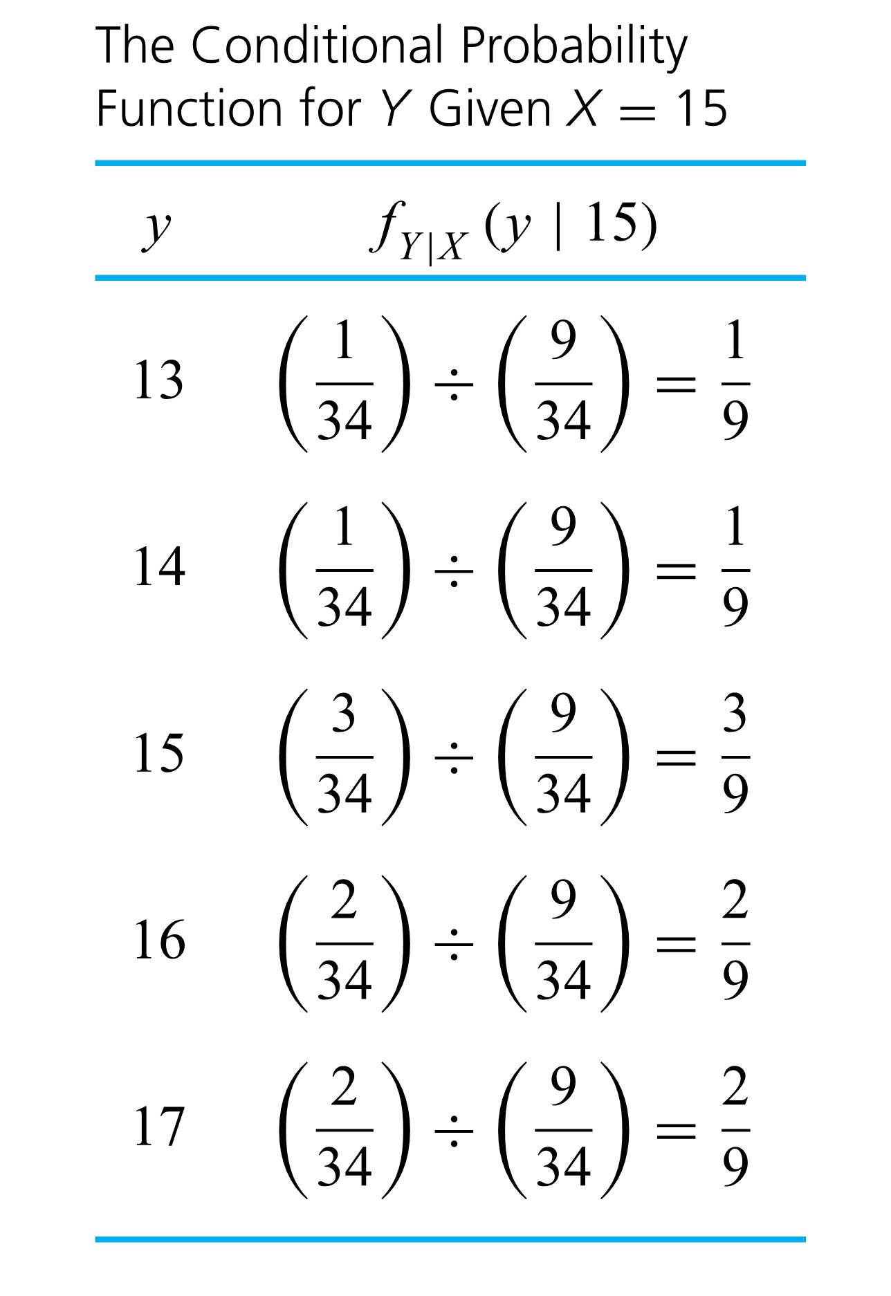
") specified by
specified by=\frac{f(18, y)}{f_{X}(18)}")
 , shown in Table 4.2.2.3 . Tables 4.2.2.2 and 4.2.4.3 confirm that the conditional distributions of
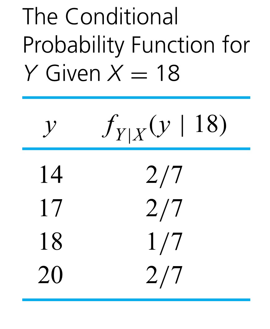
") . In this situation, equation (4.2.2.2) gives
. In this situation, equation (4.2.2.2) gives=\frac{f(x, 20)}{f_{Y}(20)}")
 row of Table 4.2.1..2 divided by the marginal
 ") is given in Table 4.2.2.4.
is given in Table 4.2.2.4.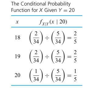
 provides some information about

 and
and =f_{U}(u)")
=f_{V}(v)")
}{f_{V}(v)}=f_{U}(u)")
=f_{U}(u) f_{V}(v)")
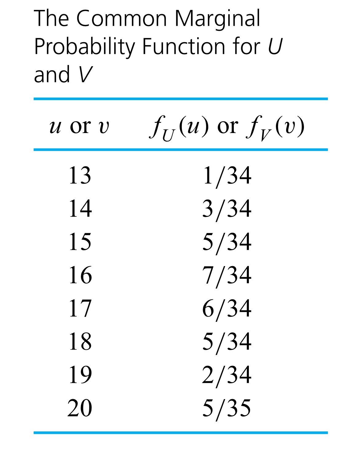
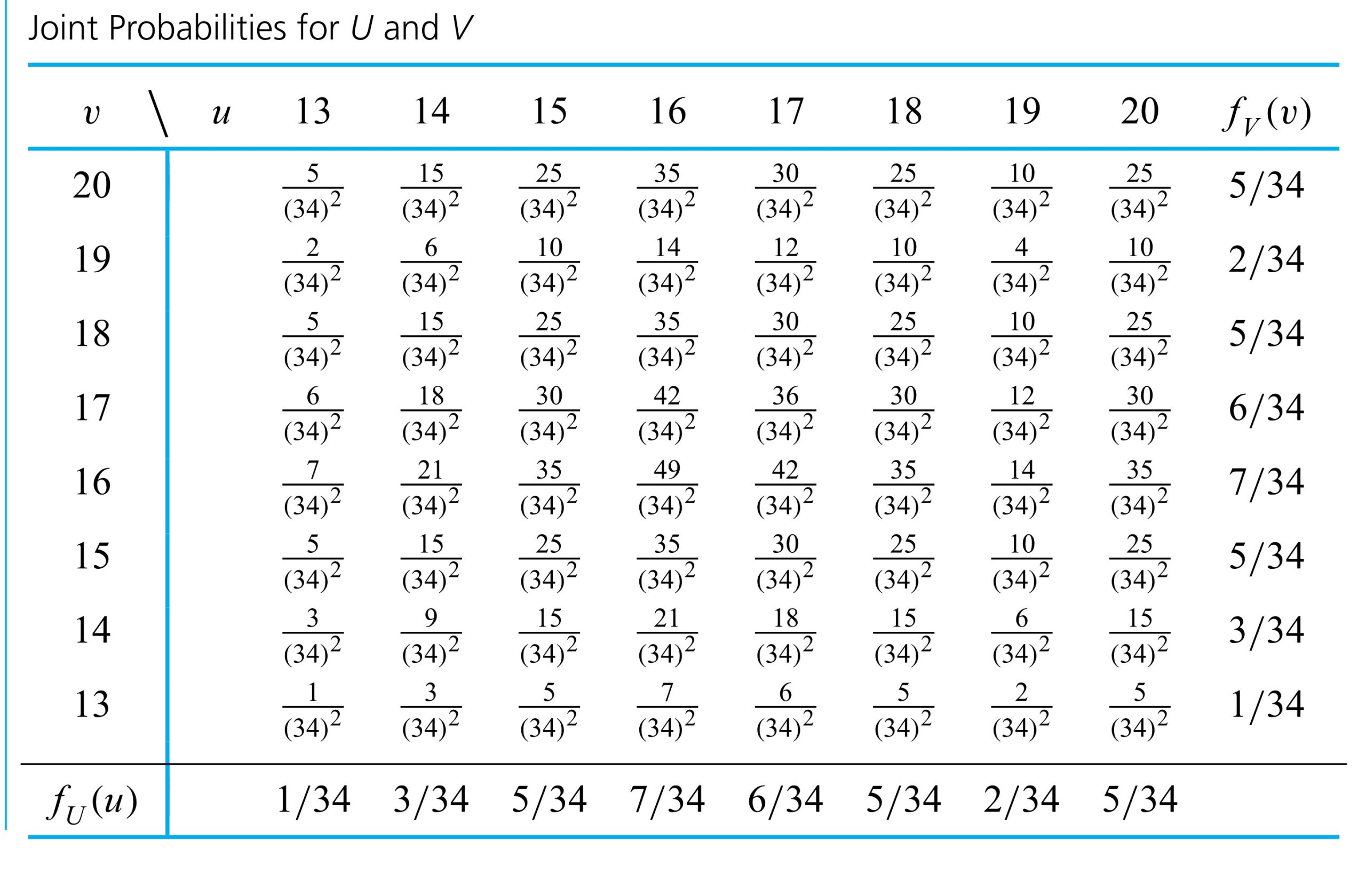
=f_{X}(x) f_{Y}(y) \quad \text { for all } x, y")
 , one clearly wants
![f(13,13)=P[U=13 \text { and } V=13]=0](https://atu0g9ctah.execute-api.ca-central-1.amazonaws.com/latest/latex?latex=f%2813%2C13%29%3DP%5BU%3D13%20%5Ctext%20%7B%20and%20%7D%20V%3D13%5D%3D0&fg=000000&font=TeX&svg=1 "f(13,13)=P[U=13 \text { and } V=13]=0")
=\frac{1}{(34)^{2}}")
=0")
=f_{V}(13)=\frac{1}{34}")
 slips labeled with torques with relative frequencies as in Table 4.2.2.6. Then even if sampling is done without replacement, the probabilities developed earlier for
 =\frac{99}{3,399}")
=\frac{f(u, v)}{f_{U}(u)}")
=f_{V \mid U}(v \mid u) f_{U}(u)")
=\frac{99}{3,399} \cdot \frac{1}{34}")

 \approx \frac{1}{34} \cdot \frac{1}{34}")
 is much larger than the sample size
  all have the same marginal distribution and are independent, they are termed iid or independent and identically distributed.
") , the object is to predict the behavior of the random variable
, the object is to predict the behavior of the random variable")


 are
are  are
are  constants, then the random variable
  has mean

 and the other
  ‘s equal to plus and minus 1 ‘s.
 , and
, and 
^{2} 6.9 \times 10^{-7}+(1)^{2} 1.04 \times 10^{-6}=1.73 \times 10^{-6}\end{aligned}")

 and [/latex]\operatorname{Var} U[/latex], there is no need to go through the intermediate step of deriving the distribution of
  . That is, in cases where random variables
=\mu")
![\begin{aligned}\operatorname{Var} \bar{X} & =\left(\frac{1}{n}\right)^{2} \operatorname{Var} X_{1}+\left(\frac{1}{n}\right)^{2} \operatorname{Var} X_{2}+\cdots+\left(\frac{1}{n}\right)^{2} \operatorname{Var} X_{n} \\& =n\left(\frac{1}{n}\right)^{2} \sigma^{2}=\frac{\sigma^{2}}{n}\end{aligned}</div> </div></blockquote> <div>.</div> <div>Since [latex]\sigma^{2} / n](https://atu0g9ctah.execute-api.ca-central-1.amazonaws.com/latest/latex?latex=%5Cbegin%7Baligned%7D%5Coperatorname%7BVar%7D%20%5Cbar%7BX%7D%20%26%20%3D%5Cleft%28%5Cfrac%7B1%7D%7Bn%7D%5Cright%29%5E%7B2%7D%20%5Coperatorname%7BVar%7D%20X_%7B1%7D%2B%5Cleft%28%5Cfrac%7B1%7D%7Bn%7D%5Cright%29%5E%7B2%7D%20%5Coperatorname%7BVar%7D%20X_%7B2%7D%2B%5Ccdots%2B%5Cleft%28%5Cfrac%7B1%7D%7Bn%7D%5Cright%29%5E%7B2%7D%20%5Coperatorname%7BVar%7D%20X_%7Bn%7D%20%5C%5C%26%20%3Dn%5Cleft%28%5Cfrac%7B1%7D%7Bn%7D%5Cright%29%5E%7B2%7D%20%5Csigma%5E%7B2%7D%3D%5Cfrac%7B%5Csigma%5E%7B2%7D%7D%7Bn%7D%5Cend%7Baligned%7D%3C%2Fdiv%3E%20%20%3C%2Fdiv%3E%3C%2Fblockquote%3E%20%20%3Cdiv%3E.%3C%2Fdiv%3E%20%20%3Cdiv%3ESince%20%5Blatex%5D%5Csigma%5E%7B2%7D%20%2F%20n&fg=000000&font=TeX&svg=1 "\begin{aligned}\operatorname{Var} \bar{X} & =\left(\frac{1}{n}\right)^{2} \operatorname{Var} X_{1}+\left(\frac{1}{n}\right)^{2} \operatorname{Var} X_{2}+\cdots+\left(\frac{1}{n}\right)^{2} \operatorname{Var} X_{n} \\& =n\left(\frac{1}{n}\right)^{2} \sigma^{2}=\frac{\sigma^{2}}{n}\end{aligned}</div> </div></blockquote> <div>.</div> <div>Since [latex]\sigma^{2} / n") is decreasing in
is decreasing in  having a probability distribution centered at the population mean
 ![\bar{X}/[latex] under random sampling with replacement, are also approximate descriptions of the behavior of [latex]\bar{X}](https://atu0g9ctah.execute-api.ca-central-1.amazonaws.com/latest/latex?latex=%5Cbar%7BX%7D%2F%5Blatex%5D%20under%20random%20sampling%20with%20replacement%2C%20are%20also%20approximate%20descriptions%20of%20the%20behavior%20of%20%5Blatex%5D%5Cbar%7BX%7D&fg=000000&font=TeX&svg=1 "\bar{X}/[latex] under random sampling with replacement, are also approximate descriptions of the behavior of [latex]\bar{X}") under simple random sampling in enumerative contexts. (Recall the discussion about the approximate independence of observations resulting from simple random sampling of large populations.)
under simple random sampling in enumerative contexts. (Recall the discussion about the approximate independence of observations resulting from simple random sampling of large populations.) .)
.) the last digit of the serial number observed next Monday at 9 A.M.
 the last digit of the serial number observed the following Monday at 9 A.M.
 is that they are independent, each with the marginal probability function
= \begin{cases}.1 & \text { if } w=0,1,2, \ldots, 9 \\ 0 & \text { otherwise }\end{cases}")
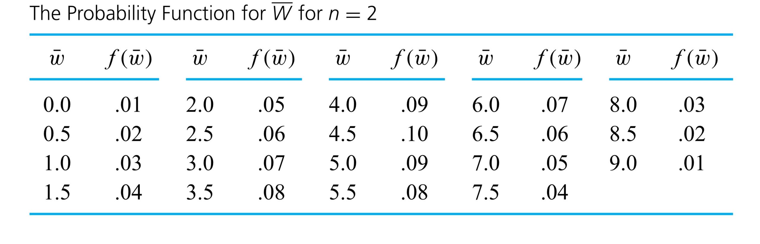
") has the probability function given in Table 4.2.2.1 and pictured in Figure 4.2.2.2
has the probability function given in Table 4.2.2.1 and pictured in Figure 4.2.2.2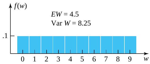
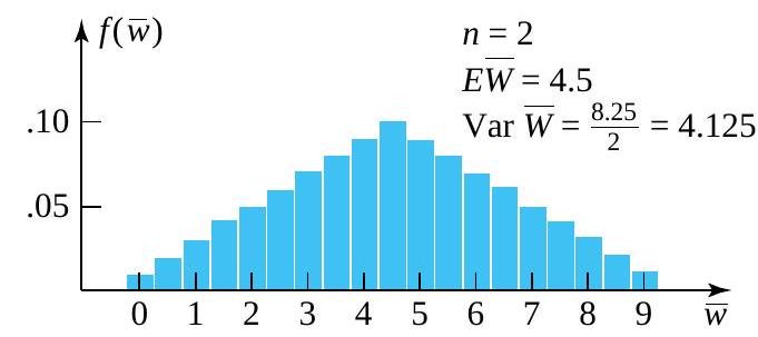
 and the small sample size of
  looks far more bell-shaped than the underlying distribution. It is clear why this is so. As you move away from the mean or central value of
  and
and  that can produce a given value of
  . For example, to observe
  , you must have
  and
and  -that is, you must observe not one but two extreme values. On the other hand, there are ten different combinations of
  .
. (with marginal distribution were simulated and each set averaged to produce 1,000 simulated values of
  . Figure 4.2.2.3 is a histogram of these 1,000 values. Notice the bell-shaped character of the plot. (The simulated mean of
  , while the variance of
  , in close agreement with formulas.)
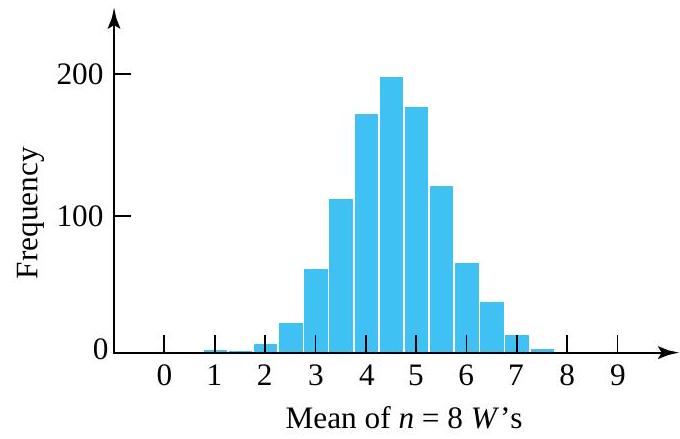
 or so is adequate to make
  excess service times, to produce
 the sample mean time (over a
  threshold) required to complete the next 100 stamp sales
![P[\bar{S}>17]](https://atu0g9ctah.execute-api.ca-central-1.amazonaws.com/latest/latex?latex=P%5B%5Cbar%7BS%7D%3E17%5D&fg=000000&font=TeX&svg=1 "P[\bar{S}>17]") .
. distribution is plausible for the individual excess service times,

 , via formulas. Further, in view of the fact that
 -values before consulting the standard normal table. In this case, the mean and standard deviation to be used are (respectively)
  and
and  . That is, a
![P[\bar{S}>17] \approx P[Z>.30]=1-\Phi(.30)=.38](https://atu0g9ctah.execute-api.ca-central-1.amazonaws.com/latest/latex?latex=P%5B%5Cbar%7BS%7D%3E17%5D%20%5Capprox%20P%5BZ%3E.30%5D%3D1-%5CPhi%28.30%29%3D.38&fg=000000&font=TeX&svg=1 "P[\bar{S}>17] \approx P[Z>.30]=1-\Phi(.30)=.38")


+(1-\Phi(2.5))=.01")
 .
.
 .It is of the same form as the corresponding null hypothesis, except that the equality sign


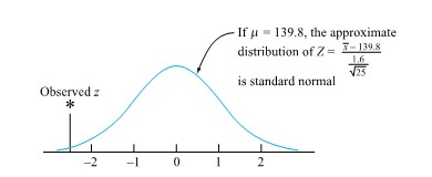
 itself. Using form (5.1.2.4), the reference distribution will always be the same—namely, standard normal.
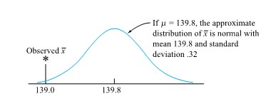
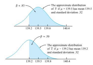
 139.8.

![\begin{aligned} & P[\text { a standard normal variable } \leq-2.5] \\ & \quad+P[\text { a standard normal variable } \geq 2.5] \\ & \quad=P[\mid \text { a standard normal variable } \mid \geq 2.5] \\ & \quad=.01 \end{aligned}](https://atu0g9ctah.execute-api.ca-central-1.amazonaws.com/latest/latex?latex=%5Cbegin%7Baligned%7D%20%26%20P%5B%5Ctext%20%7B%20a%20standard%20normal%20variable%20%7D%20%5Cleq-2.5%5D%20%5C%5C%20%26%20%5Cquad%2BP%5B%5Ctext%20%7B%20a%20standard%20normal%20variable%20%7D%20%5Cgeq%202.5%5D%20%5C%5C%20%26%20%5Cquad%3DP%5B%5Cmid%20%5Ctext%20%7B%20a%20standard%20normal%20variable%20%7D%20%5Cmid%20%5Cgeq%202.5%5D%20%5C%5C%20%26%20%5Cquad%3D.01%20%5Cend%7Baligned%7D&fg=000000&font=TeX&svg=1 "\begin{aligned} & P[\text { a standard normal variable } \leq-2.5] \\ & \quad+P[\text { a standard normal variable } \geq 2.5] \\ & \quad=P[\mid \text { a standard normal variable } \mid \geq 2.5] \\ & \quad=.01 \end{aligned}")


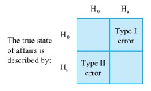
 is called the power of the significance test.

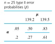
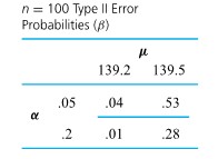


=.16")

=.02")

=\frac{\Gamma\left(\frac{v+1}{2}\right)}{\Gamma\left(\frac{v}{2}\right) \sqrt{\pi v}}\left(1+\frac{t^2}{v}\right)^{-(v+1) / 2}")
 distribution.
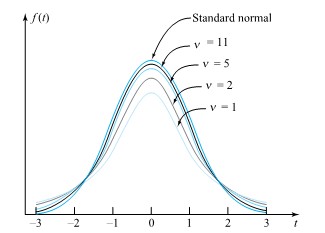
") exists. Instead, it is common to use tables (or statistical software) to evaluate common t distribution quantiles and to get at least crude bounds on the types of probabilities needed in significance testing. Table A1.2 in the Appendix 1 of statistical tables is a typical table of t quantiles. Across the top of the table are several cumulative probabilities. Down the left side are values of the degrees of freedom parameter,
exists. Instead, it is common to use tables (or statistical software) to evaluate common t distribution quantiles and to get at least crude bounds on the types of probabilities needed in significance testing. Table A1.2 in the Appendix 1 of statistical tables is a typical table of t quantiles. Across the top of the table are several cumulative probabilities. Down the left side are values of the degrees of freedom parameter, ![P[T<-1.9]=P[T>1.9]=1-P[T \leq 1.9]](https://atu0g9ctah.execute-api.ca-central-1.amazonaws.com/latest/latex?latex=P%5BT%3C-1.9%5D%3DP%5BT%3E1.9%5D%3D1-P%5BT%20%5Cleq%201.9%5D&fg=000000&font=TeX&svg=1 "P[T<-1.9]=P[T>1.9]=1-P[T \leq 1.9]")
 distribution. That is,
![P[T \leq 1.9] \leq .95](https://atu0g9ctah.execute-api.ca-central-1.amazonaws.com/latest/latex?latex=P%5BT%20%5Cleq%201.9%5D%20%5Cleq%20.95&fg=000000&font=TeX&svg=1 "P[T \leq 1.9] \leq .95")
![P[T<-1.9]<.10](https://atu0g9ctah.execute-api.ca-central-1.amazonaws.com/latest/latex?latex=P%5BT%3C-1.9%5D%3C.10&fg=000000&font=TeX&svg=1 "P[T<-1.9]<.10")
![P[T \leq 2.3]<.975](https://atu0g9ctah.execute-api.ca-central-1.amazonaws.com/latest/latex?latex=P%5BT%20%5Cleq%202.3%5D%3C.975&fg=000000&font=TeX&svg=1 "P[T \leq 2.3]<.975")


 random variable, we are in a position to work in exact analogy to what was done in Part 5 to find methods for confidence interval estimation and significance testing. That is, if a data-generating mechanism can be thought of as essentially equivalent to drawing independent observations from a single normal distribution, a two-sided confidence interval for µ has endpoints


 stress?” Since only n = 10 observations are available, the large-sample method of Part 5.1 is not applicable. Instead, only the method indicated by expression (5.2.1.5) is a possible option. For it to be appropriate, lifetimes must be normally distributed.
 distribution and chooses t > 0 such that


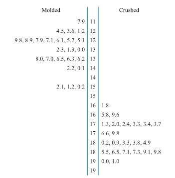
 and
and  stand for underlying distributional means corresponding to the first and second conditions and
  and
and  stand for corresponding sample means. Now if the two data-generating mechanisms are conceptually essentially equivalent to sampling with replacement from two distributions, Part 4 says that
  and
and  . The difference in sample means
 =\mu_1-\mu_2")
=\frac{\sigma_1^2}{n_1}+\frac{\sigma_2^2}{n_2}")
 and
and  are large (so that
 }{\sqrt{\frac{\sigma_1^2}{n_1}+\frac{\sigma_2^2}{n_2}}}")
 and
and  . Happily, for large
 }{\sqrt{\frac{s_1^2}{n_1}+\frac{s_2^2}{n_2}}}")


 = 8.34 g,
  = 9.31 g, the five-step testing format produces the following summary:


^2}{24}+\frac{(9.31)^2}{24}}}=18.3")
-1.645 \sqrt{\frac{(8.34)^2}{24}+\frac{(9.31)^2}{24}}")

")
")
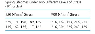


 and
and  ,the pooled sample variance,
  s_1^2+\left(n_2-1\right) s_2^2}{\left(n_1-1\right)+\left(n_2-1\right)}=\frac{\left(n_1-1\right) s_1^2+\left(n_2-1\right) s_2^2}{n_1+n_2-2}")
 , is the square root of
 (42.9)^2+(10-1)(33.1)^2}{(10-1)+(10-1)}=1,468\left(10^3 \text { cycles }\right)^2")
")
}{\sigma \sqrt{\frac{1}{n_1}+\frac{1}{n_2}}}")
-\left(\mu_1-\mu_2\right)}{s_{\mathrm{P}} \sqrt{\frac{1}{n_1}+\frac{1}{n_2}}}")


 distribution assigns to the interval between −t and t corresponds to the desired confidence. And under the same conditions,
 mm^2 stress level condition 1 and the 950 N/


 distribution is in order. Endpoints of the confidence interval for
  \pm 2.101(38.3) \sqrt{\frac{1}{10}+\frac{1}{10}}")


^2}{\frac{s_1^4}{\left(n_1-1\right) n_1^2}+\frac{s_2^4}{\left(n_2-1\right) n_2^2}}")
 is such that the
  degrees of freedom assigns that probability to the interval between
  and
and 
^2}{10}+\frac{(33.1)^2}{10}\right)^2}{\frac{(57.9)^4}{9(100)}+\frac{(33.1)^4}{9(100)}}=14.3")
 distribution is 2.145. So the 95% limits (5.3.3.8) for the (850 N/
 −
−  )are
)are^2}{10}+\frac{(33.1)^2}{10}}")


 distribution with numerator and denominator degrees of freedom parameters
  and
and  is a continuous probability distribution with probability density
= \begin{cases}\frac{\Gamma\left(\frac{v_1+v_2}{2}\right)\left(\frac{v_1}{v_2}\right)^{v_1 / 2} x^{\left(v_1 / 2\right)-1}}{\Gamma\left(\frac{v_1}{2}\right) \Gamma\left(\frac{v_2}{2}\right)\left(1+\frac{v_1 x}{v_2}\right)^{\left(v_1+v_2\right) / 2}} & \text { for } x>0 \\ 0 & \text { otherwise }\end{cases}")
 distribution.
 (the numerator degrees of freedom) and
  (the denominator degrees of freedom). The values of
  and
and  quantiles, quantiles for small
  stand for the
  stand for the quantile function for the
 =\frac{1}{Q_{v_{2}, v_{1}}(1-p)}")

 random variable. Consider finding the .95 and .01 quantiles of
  4.0] and
 ![P[V<.3]](https://atu0g9ctah.execute-api.ca-central-1.amazonaws.com/latest/latex?latex=P%5BV%3C.3%5D&fg=000000&font=TeX&svg=1 "P[V<.3]") .
. table of quantiles, in the
  column and
  row, produces the number 5.41. That is,
 =5.41") , or (equivalently)
, or (equivalently) ![P[V<5.41]=.95](https://atu0g9ctah.execute-api.ca-central-1.amazonaws.com/latest/latex?latex=P%5BV%3C5.41%5D%3D.95&fg=000000&font=TeX&svg=1 "P[V<5.41]=.95") .
. quantile of the
 =\frac{1}{Q_{5,3}(.99)}")
 column and
  row of the table of
  quantiles, one has
=\frac{1}{28.24}=.04")
![P[V>4.0]](https://atu0g9ctah.execute-api.ca-central-1.amazonaws.com/latest/latex?latex=P%5BV%3E4.0%5D&fg=000000&font=TeX&svg=1 "P[V>4.0]") , one finds (using the [/latex]v_{1}=3[/latex] columns and
, one finds (using the [/latex]v_{1}=3[/latex] columns and  ), in the
  distribution and then make use of expression (5.2.4.2). Using the
  and
and  of those underlying distributions. That is, when
  and
and ![s_{2}^{2}[latex] come from independent samples from normal distributions, the variable <blockquote> <p style="text-align: left"><strong>5.2.4.3 </strong> [latex]F=\frac{s_{1}^{2}}{\sigma_{1}^{2}} \cdot \frac{\sigma_{2}^{2}}{s_{2}^{2}}](https://atu0g9ctah.execute-api.ca-central-1.amazonaws.com/latest/latex?latex=s_%7B2%7D%5E%7B2%7D%5Blatex%5D%20come%20from%20independent%20samples%20from%20normal%20distributions%2C%20the%20variable%20%20%3Cblockquote%3E%20%20%3Cp%20style%3D%22text-align%3A%20left%22%3E%3Cstrong%3E5.2.4.3%C2%A0%20%C2%A0%20%C2%A0%20%C2%A0%20%C2%A0%20%C2%A0%20%C2%A0%20%C2%A0%20%C2%A0%20%C2%A0%3C%2Fstrong%3E%20%5Blatex%5DF%3D%5Cfrac%7Bs_%7B1%7D%5E%7B2%7D%7D%7B%5Csigma_%7B1%7D%5E%7B2%7D%7D%20%5Ccdot%20%5Cfrac%7B%5Csigma_%7B2%7D%5E%7B2%7D%7D%7Bs_%7B2%7D%5E%7B2%7D%7D&fg=000000&font=TeX&svg=1 "s_{2}^{2}[latex] come from independent samples from normal distributions, the variable <blockquote> <p style="text-align: left"><strong>5.2.4.3 </strong> [latex]F=\frac{s_{1}^{2}}{\sigma_{1}^{2}} \cdot \frac{\sigma_{2}^{2}}{s_{2}^{2}}")
 distribution. (
  associated degrees of freedom and is in the numerator of this expression, while
  has
has  associated degrees of freedom and is in the denominator, providing motivation for the language introduced in Definition 5.2.4.1)
 . For example, it is possible to pick appropriate F quantiles L and U such that the probability that the variable (5.2.4.3) falls between L and U corresponds to a desired confidence level. (Typically, L and U are chosen to "split the 'unconfidence' " between the upper and lower
  <U
<U


 in displays (5.2.4.5) and (5.2.4.6), so that the null hypothesis is one of equality of variances, is the only one commonly used in practice.)
 < # and
  are (respectively) the left and right
  , the standard convention is to report twice the
  if
if  and to report twice the
  carbon steel. Part of their data are given in Table 5.2.4.1, where Rockwell hardness measurements for ten specimens from a lot of heat-treated steel specimens and five specimens from a lot of cold-rolled steel specimens are represented.
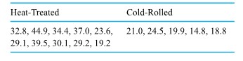


 and
and  , and a five-step significance test of equality of variances based on the variable (5.2.4.6) proceeds as follows:
![]\mathrm{H}_{0}: \frac{\sigma_{1}^{2}}{\sigma_{2}^{2}}=1](https://atu0g9ctah.execute-api.ca-central-1.amazonaws.com/latest/latex?latex=%5D%5Cmathrm%7BH%7D_%7B0%7D%3A%20%5Cfrac%7B%5Csigma_%7B1%7D%5E%7B2%7D%7D%7B%5Csigma_%7B2%7D%5E%7B2%7D%7D%3D1&fg=000000&font=TeX&svg=1 "]\mathrm{H}_{0}: \frac{\sigma_{1}^{2}}{\sigma_{2}^{2}}=1")


 distribution, and both large observed f and small observed f will constitute evidence against
  .
.^{2}}{(3.52)^{2}}=4.6")
![2 P\left[\text { an } F_{9,4} \text { random variable } \geq 4.6\right]](https://atu0g9ctah.execute-api.ca-central-1.amazonaws.com/latest/latex?latex=2%20P%5Cleft%5B%5Ctext%20%7B%20an%20%7D%20F_%7B9%2C4%7D%20%5Ctext%20%7B%20random%20variable%20%7D%20%5Cgeq%204.6%5Cright%5D&fg=000000&font=TeX&svg=1 "2 P\left[\text { an } F_{9,4} \text { random variable } \geq 4.6\right]")
 . Now the .95 quantile of the
  distribution is 3.63, implying that the .05 quantile of the
  . Thus, a 90 % confidence interval for the ratio of standard deviations
 ^{2}}{6.0(3.52)^{2}}} \text { and } \sqrt{\frac{(7.52)^{2}}{(1 / 3.63)(3.52)^{2}}}")
 /
/ to be on the order of 1.5 and predicted a period of two years or less for the recovery of the capital improvement cost of equipping all the company’s ream cutters with automatic brakes.
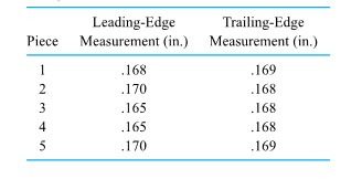
 , if n (the number of data pairs) is large, endpoints of a confidence interval for the underlying mean difference,
  , are
, are
 is the sample standard deviation of d1 , d2 ,…,


 =−.0008 in. and
  = .0023 in. So, first investigating the plausibility of a “no consistent difference” hypothesis in a five-step significance testing format, gives the following:

 random variable|≥.78], which can be seen from Table A1.2 to be larger than 2(.10) = .2. The data in hand are not convincing in favor of a systematic difference between leading- and trailing-edge measurements.
 =−.0008, is just a result of sampling variability.
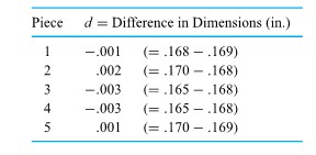
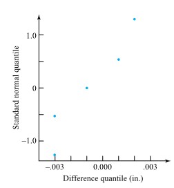
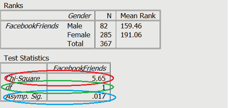
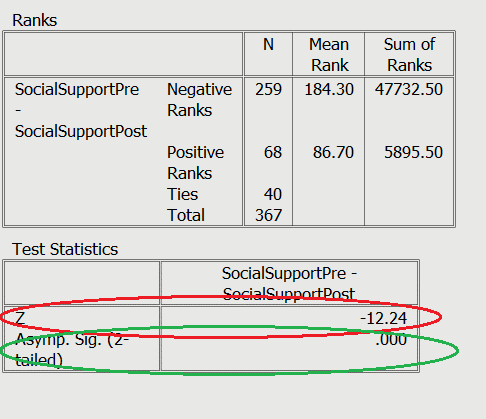
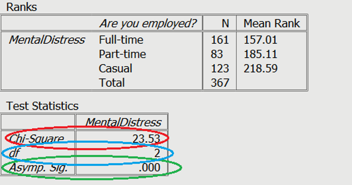

 amounts to making a scatterplot of compressive strength versus formula number. Such a plot is shown in Figure 6.1.1.1. The general message conveyed by Figure 6.1.1.1 is that there are clear differences in mean compressive strengths between the formulas but that the variabilities in compressive strengths are roughly comparable for the eight different formulas.
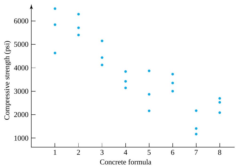
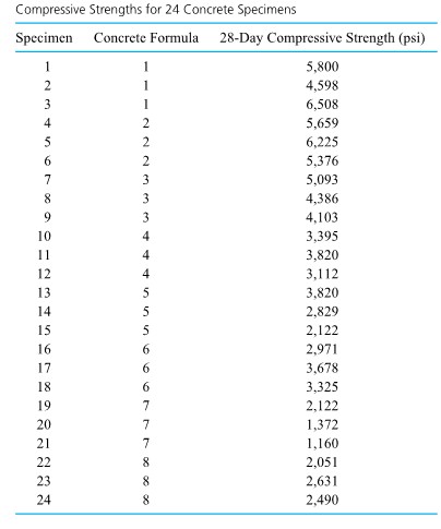
 springs of type 1 (a 4 in. design with a theoretical spring constant of 1.86),
  springs of type 2 (a 6 in. design with a theoretical spring constant of 2.63), and
  springs of type 3 (a 4 in. design with a theoretical spring constant of 2.12), using an
  load. The students’ experimental values are given in Table 6.1.1.2
 . spring types but that no such difference between the two 4 in. spring types is obvious. Of course, the information in Table 6.1.1.2 could also be presented in side-by-side dot diagram form, as in Figure 6.1.1.3.
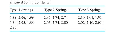
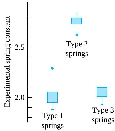
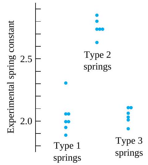
 samples of respective sizes
  are independent samples from normal underlying distributions with a common variance-say,
  version of this one-way (as opposed, for example, to several-way factorial) model led to useful inference methods for
  , this general version will support a variety of useful inference methods for


 is the
  ,
,  are independent normal random variables with mean 0 and variance
  and the variance


 deterministic response + noise
 ") are meant to approximate the deterministic part of a system response
are meant to approximate the deterministic part of a system response ") , and
, and") are therefore meant to approximate the corresponding noise in the response
are therefore meant to approximate the corresponding noise in the response ") .
. in equation (6.1.2.1) are assumed to be iid normal
 ") random variables then suggests that the
random variables then suggests that the  ought to look at least approximately like a random sample from a normal distribution.
 is more than three times the size of
  . But the sample sizes here are so small that a largest ratio of sample standard deviations on the order of 3.2 is hardly unusual (for
  samples of size 3 from a normal distribution). Note from the
 ^{2} \approx 10.2") would yield a
would yield a  residuals. Some of the calculations necessary to compute residuals for the data in Table 6.1.1.1 (using the fitted values appearing as sample means in Table 6.1.2.1) are shown in Table 6.1.2.2. Figures 6.1.2.2 and 6.1.2.3 are, respectively, a plot of residuals versus fitted
  versus
  ) and a normal plot of all 24 residuals.
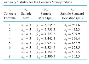

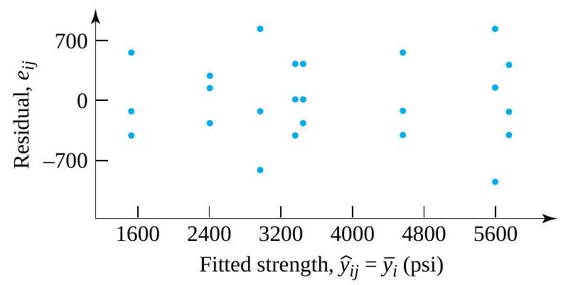
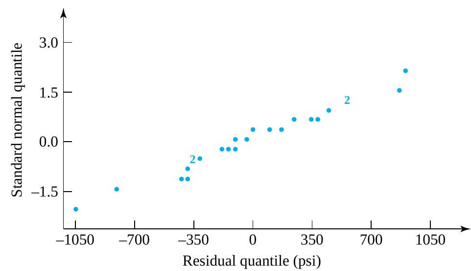
^{2}=4.38\right)") is not a compelling reason to abandon a one-way model description of the spring constants. (A look at the
is not a compelling reason to abandon a one-way model description of the spring constants. (A look at the  and
and  distribution .9 and .95 quantiles. So even if there were only two rather than three samples involved, a variance ratio of 4.38 would yield a
  are large enough that it makes sense to look at sample-by-sample normal plots of the spring constant data. Such plots, drawn on the same set of axes, are shown in Figure 6.1.2.4. Further, use of the fitted values
 ") listed in Table 6.1.2.3 with the original data given in Table 6.1.1.2 produces 19 residuals, as partially illustrated in Table 6.1.2.4. Then Figures 6.1.2.5 and 6.1.2.6, respectively, show a plot of residuals versus fitted responses and a normal plot of all 19 residuals.
listed in Table 6.1.2.3 with the original data given in Table 6.1.1.2 produces 19 residuals, as partially illustrated in Table 6.1.2.4. Then Figures 6.1.2.5 and 6.1.2.6, respectively, show a plot of residuals versus fitted responses and a normal plot of all 19 residuals.
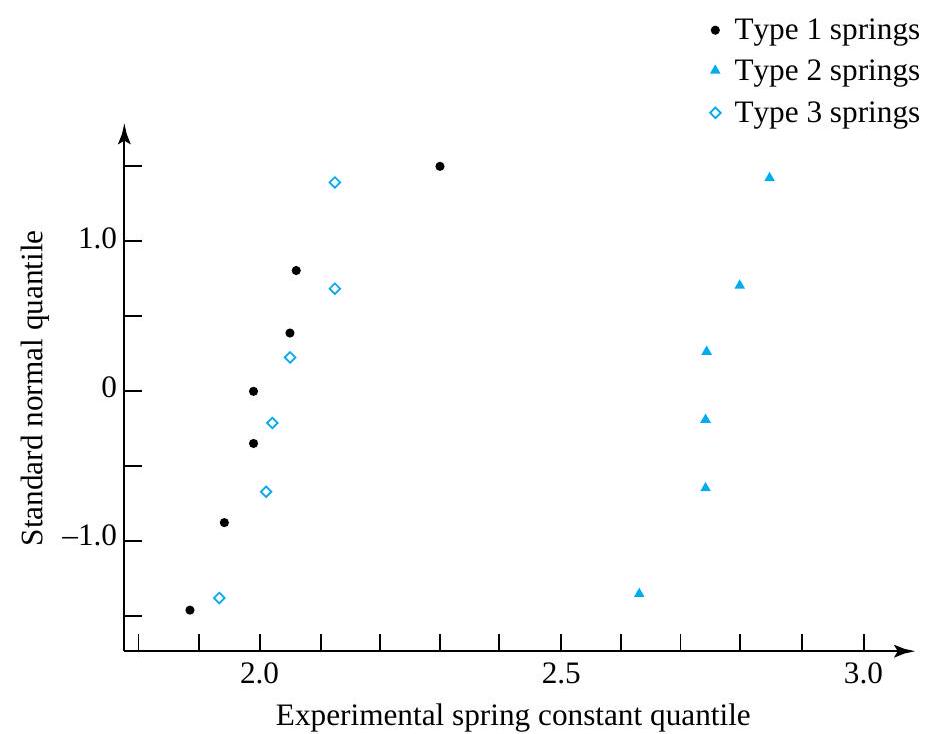

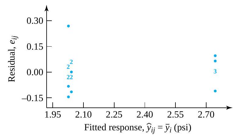
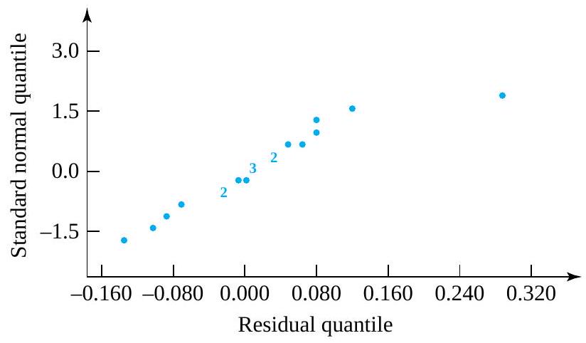
 . Similar to what was done in the
  , the pooled sample variance,
  , is the weighted average of the sample variances, where the weights are the sample sizes minus 1 . That is,
s_{1}^{2}+\left(n_{2}-1\right) s_{2}^{2}+\cdots+\left(n_{r}-1\right) s_{r}^{2}}{\left(n_{1}-1\right)+\left(n_{2}-1\right)+\cdots+\left(n_{r}-1\right)}")
 , is the square root of
  .
. based on two samples,
  and is a mathematically convenient form of compromise value.
=\sum_{i=1}^{r} n_{i}-\sum_{i=1}^{r} 1=n-r")
^{2}")
\left(\frac{1}{\left(n_{i}-1\right)} \sum_{j=1}^{n_{i}}\left(y_{i j}-\bar{y}_{i}\right)^{2}\right) & =\sum_{i=1}^{r} \sum_{j=1}^{n_{i}}\left(y_{i j}-\bar{y}_{i}\right)^{2} \\& =\sum_{i=1}^{r} \sum_{j=1}^{n_{i}} e_{i j}^{2}\end{aligned}")

 .
. are 3 , and
 ![\begin{aligned} s_{\mathrm{P}}^{2} & =\frac{(3-1)(965.6)^{2}+(3-1)(432.3)^{2}+\cdots+(3-1)(302.5)^{2}}{(3-1)+(3-1)+\cdots+(3-1)} \\ & =\frac{2\left[(965.6)^{2}+(432.3)^{2}+\cdots+(302.5)^{2}\right]}{16} \\ & =\frac{2,705,705}{8} \\ & =338,213(\mathrm{psi})^{2} \end{aligned}](https://atu0g9ctah.execute-api.ca-central-1.amazonaws.com/latest/latex?latex=%5Cbegin%7Baligned%7D%20s_%7B%5Cmathrm%7BP%7D%7D%5E%7B2%7D%20%26%20%3D%5Cfrac%7B%283-1%29%28965.6%29%5E%7B2%7D%2B%283-1%29%28432.3%29%5E%7B2%7D%2B%5Ccdots%2B%283-1%29%28302.5%29%5E%7B2%7D%7D%7B%283-1%29%2B%283-1%29%2B%5Ccdots%2B%283-1%29%7D%20%5C%5C%C2%A0%26%20%3D%5Cfrac%7B2%5Cleft%5B%28965.6%29%5E%7B2%7D%2B%28432.3%29%5E%7B2%7D%2B%5Ccdots%2B%28302.5%29%5E%7B2%7D%5Cright%5D%7D%7B16%7D%20%5C%5C%C2%A0%26%20%3D%5Cfrac%7B2%2C705%2C705%7D%7B8%7D%20%5C%5C%C2%A0%26%20%3D338%2C213%28%5Cmathrm%7Bpsi%7D%29%5E%7B2%7D%C2%A0%5Cend%7Baligned%7D&fg=000000&font=TeX&svg=1 "\begin{aligned} s_{\mathrm{P}}^{2} & =\frac{(3-1)(965.6)^{2}+(3-1)(432.3)^{2}+\cdots+(3-1)(302.5)^{2}}{(3-1)+(3-1)+\cdots+(3-1)} \\ & =\frac{2\left[(965.6)^{2}+(432.3)^{2}+\cdots+(302.5)^{2}\right]}{16} \\ & =\frac{2,705,705}{8} \\ & =338,213(\mathrm{psi})^{2} \end{aligned}")


 s_{\mathrm{P}}^{2}}{\sigma^{2}}")
 distribution. Thus, in a manner exactly parallel to the derivation in Part 5, a two-sided confidence interval for
 ![\sigma^{2}[latex] has endpoints</div> <div style="text-align: left">.</div> <blockquote> <div style="text-align: left"><strong>6.1.3.4 </strong>[latex]\frac{(n-r) s_{\mathrm{P}}^{2}}{U} \text { and } \frac{(n-r) s_{\mathrm{P}}^{2}}{L}](https://atu0g9ctah.execute-api.ca-central-1.amazonaws.com/latest/latex?latex=%5Csigma%5E%7B2%7D%5Blatex%5D%20has%20endpoints%3C%2Fdiv%3E%20%3Cdiv%20style%3D%22text-align%3A%20left%22%3E.%3C%2Fdiv%3E%20%3Cblockquote%3E%20%3Cdiv%20style%3D%22text-align%3A%20left%22%3E%3Cstrong%3E6.1.3.4%C2%A0%20%C2%A0%20%C2%A0%20%C2%A0%20%C2%A0%20%3C%2Fstrong%3E%5Blatex%5D%5Cfrac%7B%28n-r%29%20s_%7B%5Cmathrm%7BP%7D%7D%5E%7B2%7D%7D%7BU%7D%20%5Ctext%20%7B%20and%20%7D%20%5Cfrac%7B%28n-r%29%20s_%7B%5Cmathrm%7BP%7D%7D%5E%7B2%7D%7D%7BL%7D&fg=000000&font=TeX&svg=1 "\sigma^{2}[latex] has endpoints</div> <div style="text-align: left">.</div> <blockquote> <div style="text-align: left"><strong>6.1.3.4 </strong>[latex]\frac{(n-r) s_{\mathrm{P}}^{2}}{U} \text { and } \frac{(n-r) s_{\mathrm{P}}^{2}}{L}")
 and
and ") is the desired confidence level. And, of course, a one-sided interval is available by using only one of the endpoints (6.1.3.4) and choosing
is the desired confidence level. And, of course, a one-sided interval is available by using only one of the endpoints (6.1.3.4) and choosing ") is the desired confidence.
is the desired confidence. confidence interval for
  degrees of freedom are associated with
  distribution. These are 7.962 and 26.296, respectively. Thus a confidence interval for
 ^{2}}{26.296} \text { and } \frac{16(581.6)^{2}}{7.962}")
^{2}}{26.296}} \text { and } \sqrt{\frac{16(581.6)^{2}}{7.962}}")


 distribution. Hence, a two-sided confidence interval for the
 to
to  to
to  , the variable
}{s_{\mathrm{P}} \sqrt{\frac{1}{n_{i}}+\frac{1}{n_{i^{\prime}}}}}")
 has endpoints
 .
.") (for
(for  ). The virtues of formulas (6.2.1.1) and (6.2.1.2) (in comparison to the corresponding formulas from Part 5) are that (when appropriate) for a given confidence, they will tend to produce shorter intervals than their Part 5 counterparts.
 and
and  . So the .95 quantile of the
  distribution, namely 1.746, is appropriate for use in both formulas (6.2.1.1) and (6.2.1.2).
 is 3 , the plus-or-minus part of formula (6.2.1.1) gives
 psi precision could be attached to any one of the sample means in Table 6.2.1.1 as an estimate of the corresponding formula’s mean strength. For example, since
  psi, a
  has endpoints

 \sqrt{\frac{1}{3}+\frac{1}{3}}=829.1 \mathrm{psi}")
 psi precision could be attached to any difference between sample means in Table 6.2.1.1 as an estimate of the corresponding difference in formula mean strengths. For instance, since
  , a
, a  has endpoints
 \pm 829.1")

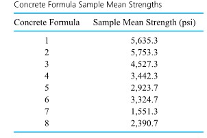
 and
and  reflects the reduction in uncertainty associated with
 ")
 confidence intervals have associated confidences
  , the Bonferroni inequality says that the simultaneous or joint confidence that all
  ) satisfies
+\left(1-\gamma_{2}\right)+\cdots+\left(1-\gamma_{k}\right)\right)")
") is no larger than the sum of the
is no larger than the sum of the  confidence levels have a joint or simultaneous confidence level of at least 95%.)
}{2}") pairs of mean responses
pairs of mean responses  . Section 6.2 argued thata single difference in mean responses,
  versus
  versus
  versus
  versus
  , and
, and  versus
  ). If one wishes to guarantee a reasonable simultaneous confidence level for all these comparisons via the crude Bonferroni idea, a huge individual confidence level is required for the intervals (6.2.3.1). For example, the Bonferroni inequality requires
  individual confidence for 28 intervals in order to guarantee simultaneous
  confidence.
 such that the set of two-sided intervals with endpoints
 ) is read from Table A5A or
  .99) is read from Table A5B) in the estimation of all differences
  ).
). \sqrt{\frac{1}{3}+\frac{1}{3}}")

 \sqrt{\frac{1}{3}+\frac{1}{3}}")

 row of Table A5A.)
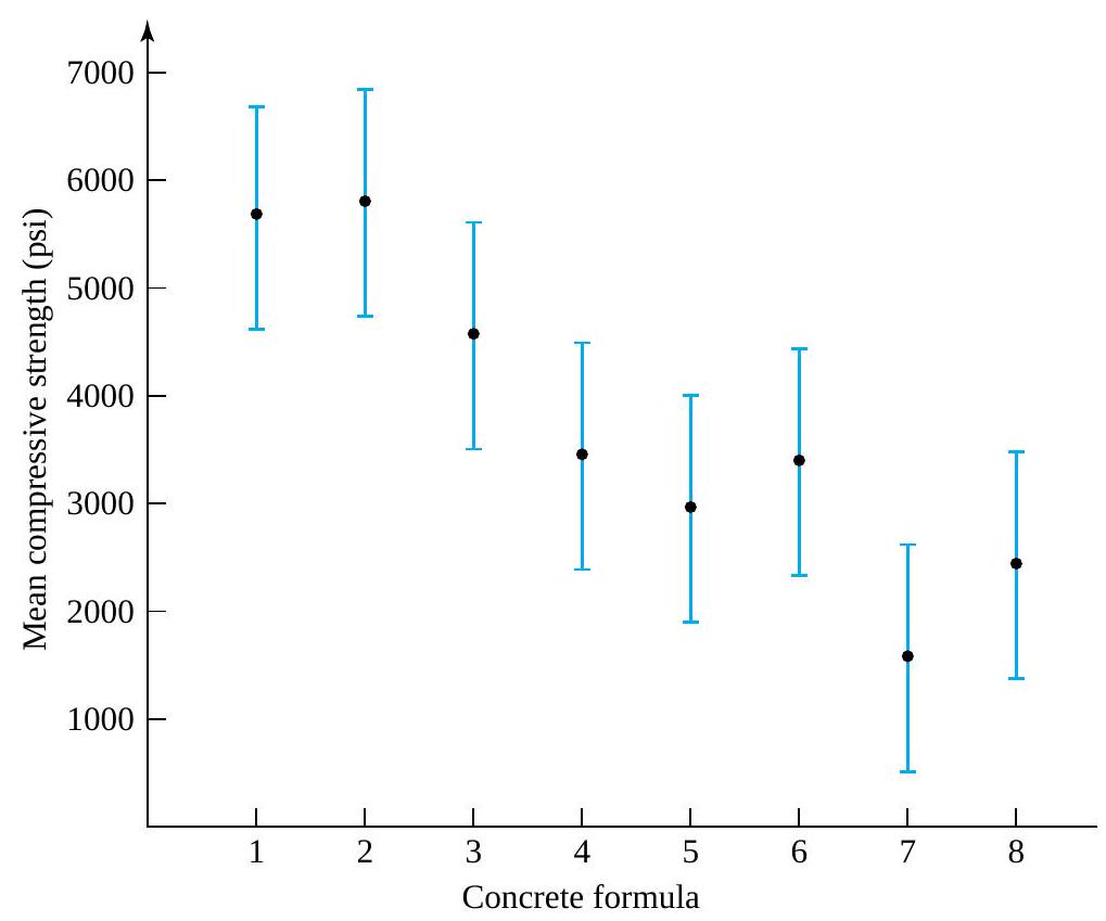


=0")


 and \#.


 , the number of observations in hand ignoring the fact that
  for the grand sample average of response
 but is a weighted average of the sample means
  . On the other hand,
  , and
, and  ,
,=\frac{2}{5} \bar{y}_{1}+\frac{3}{5} \bar{y}_{2}")
=\frac{1}{4} y_{11}+\frac{1}{4} y_{12}+\frac{1}{6} y_{21}+\frac{1}{6} y_{22}+\frac{1}{6} y_{23}")
 is a natural estimate of the common mean. (All underlying distributions are the same, so the data in hand are reasonably thought of not as
  are indicators of possible differences among the
 ^{2}")
 or as an unweighted sum, where there is a term in the sum for each raw data point and therefore
or as an unweighted sum, where there is a term in the sum for each raw data point and therefore  s_{\mathrm{p}}^{2}") , giving
, giving^{2}}{s_{\mathrm{P}}^{2}}")
 distribution. So the hypothesis of equality of
  : not
: not  and the 8 sample means
  , in this situation,
^2= & 3(1,941.7)^2+3(2,059.7)^2+\cdots \\ & +3(-2,142.3)^2+3(-1,302.9)^2 \end{aligned}")
^{2}")
}{(581.6)^{2}}=20.0")
 distribution. So
![p \text {-value }=P\left[\text { an } F_{7,16} \text { random variable } \geq 20.0\right]<.001](https://atu0g9ctah.execute-api.ca-central-1.amazonaws.com/latest/latex?latex=p%20%5Ctext%20%7B-value%20%7D%3DP%5Cleft%5B%5Ctext%20%7B%20an%20%7D%20F_%7B7%2C16%7D%20%5Ctext%20%7B%20random%20variable%20%7D%20%5Cgeq%2020.0%5Cright%5D%3C.001&fg=000000&font=TeX&svg=1 "p \text {-value }=P\left[\text { an } F_{7,16} \text { random variable } \geq 20.0\right]<.001")
 are not all equal.
 s^{2}=\sum_{i=1}^{r} n_{i}\left(\bar{y}_{i}-\bar{y}\right)^{2}+(n-r) s_{\mathrm{P}}^{2}")
^{2}=\sum_{i=1}^{r} n_{i}\left(\bar{y}_{i}-\bar{y}\right)^{2}+\sum_{i=1}^{r} \sum_{j=1}^{n_{i}}\left(y_{i j}-\bar{y}_{i}\right)^{2}")
 s^{2}=\sum_{i, j}\left(y_{i j}-\bar{y}\right)^{2}")
 s_{\mathrm{P}}^{2}=\sum_{i=1}^{r} \sum_{j=1}^{n_{i}}\left(y_{i j}-\bar{y}_{i}\right)^{2}")
 s^{2}") , the sum of squared differences between the raw data values and the grand sample mean, will be called the total sum of squares and denoted as SSTot.
, the sum of squared differences between the raw data values and the grand sample mean, will be called the total sum of squares and denoted as SSTot.^{2}") will be called the treatment sum of squares and denoted as SSTr.
will be called the treatment sum of squares and denoted as SSTr.^{2}") (which is
(which is  s_{\mathrm{p}}^{2}") in the unstructured situation) will be called the error sum of squares and denoted as SSE.
in the unstructured situation) will be called the error sum of squares and denoted as SSE.
 of
of  (corresponding to the source), degrees of freedom (corresponding to the source), Mean Square (corresponding to the source), and
  (for testing the significance of the source in contributing to the overall observed variability). The entries in the Source column of the table are shown here as being Treatments, Error, and Total. But the name Treatments is sometimes replaced by Between (Samples), and the name Error is sometimes replaced by Within (Samples) or Residual. The first two entries in the SS column must sum to the third, as indicated in equation (6.3.3.3). Similarly, the Treatments and Error degrees of freedom add to the Total degrees of freedom,
 ") . Notice that the entries in the
. Notice that the entries in the  column are those attached to the numerator and denominator, respectively, of the test statistic in equation (6.3.2.3). The ratios of sums of squares to degrees of freedom are called mean squares, here the mean square for treatments (MSTr) and the mean square for error (MSE). Verify that in the present context,
  and
and  is the numerator of the
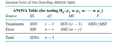
 s^2 \\ = & (5,800-3,693.6)^2+(4,598-3,693.6)^2+(6,508-3,693.6)^2 \\ & +\cdots+(2,631-3,693.6)^2+(2,490-3,693.6)^2 \\ = & 52,772,190(\mathrm{psi})^2 \end{aligned}")
^{2}") and
and  s_{\mathrm{P}}^{2}=5,411,410(\mathrm{psi})^{2}")
^{2}=47,360,780")
 .
.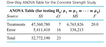
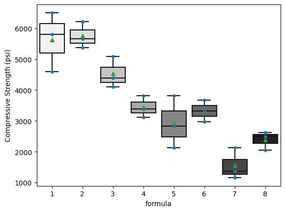
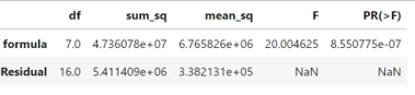
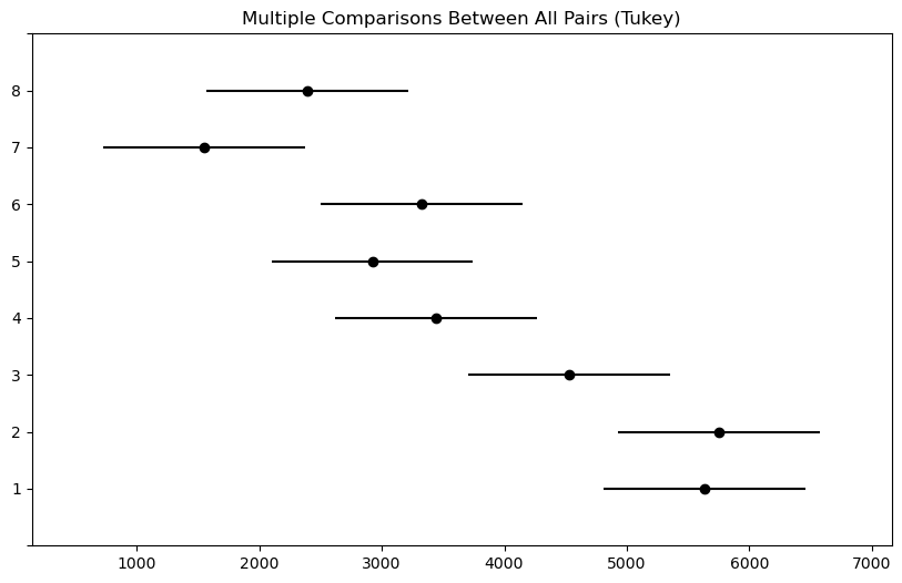

 , polyvinyl alcohol, and water was prepared, dried overnight, crushed, and sieved to obtain 100 mesh size grains. These were pressed into cylinders at pressures from 2,000 psi to 10,000 psi, and cylinder densities were calculated. Table 7.1.1.1 gives the data that were obtained, and a simple scatterplot of these data is given in Figure 7.1.1.1.
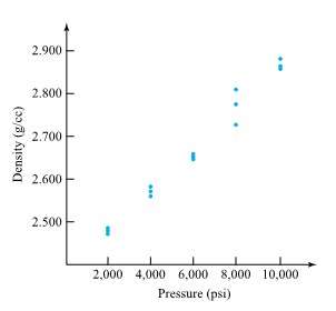

^2")
 are the observed responses and
  are corresponding responses predicted or fitted by the equation.
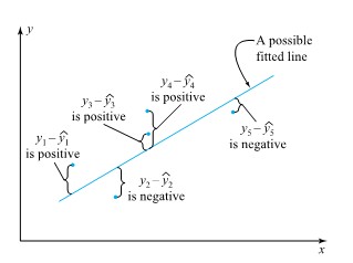

") and intercept
and intercept ") is
is=\sum_{i=1}^n\left(y_i-\left(\beta_0+\beta_1 x_i\right)\right)^2")
") is an exercise in calculus. The partial derivatives of
is an exercise in calculus. The partial derivatives of  and
and  may be set equal to zero, and the two resulting equations may be solved simultaneously for
  \beta_1=\sum_{i=1}^n y_i")
 \beta_0+\left(\sum_{i=1}^n x_i^2\right) \beta_1=\sum_{i=1}^n x_i y_i")
\left(y_i-\bar{y}\right)}{\sum\left(x_i-\bar{x}\right)^2}")

 and
and .
.^2= & (2,000-6,000)^2+(2,000-6,000)^2+\cdots+ \\ \sum y_i= & 2.486+2.479+\cdots+2.858=40.005, \\ \text { so } \bar{y}= & \frac{40.005}{15}=2.667 \\ \sum\left(y_i-\bar{y}\right)^2= & (2.486-2.667)^2+(2.479-2.667)^2+\cdots+ \\ & (2.858-2.667)^2=.289366 \\ \sum\left(x_i-\bar{x}\right)\left(y_i-\bar{y}\right)= & (2,000-6,000)(2.486-2.667)+\cdots+ \\ & (10,000-6,000)(2.858-2.667)=5,840 \end{aligned}")
 / \mathrm{psi}")
(6,000)=2.375 \mathrm{~g} / \mathrm{cc}")

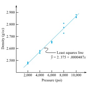
=2.5693 \mathrm{~g} / \mathrm{cc}")
=2.5697 \mathrm{~g} / \mathrm{cc}")
=2.6183 \mathrm{~g} / \mathrm{cc}")
") is
is\left(y_i-\bar{y}\right)}{\sqrt{\sum\left(x_i-\bar{x}\right)^2 \cdot \sum\left(y_i-\bar{y}\right)^2}}")
^2 / \sum\left(y_i-\bar{y}\right)^2\right)^{1 / 2}") so that
so that (.289366)}}=.9911")
^2-\sum\left(y_i-\hat{y}_i\right)^2}{\sum\left(y_i-\bar{y}\right)^2}")

^2 \geq \sum\left(y_i-\hat{y}_i\right)^2") . Further,
. Further, ^2") is a measure of raw variability in y, while
is a measure of raw variability in y, while ^2") is a measure of variation in y remaining after fitting the equation. So the nonnegative difference
is a measure of variation in y remaining after fitting the equation. So the nonnegative difference ^2-\sum\left(y_i-\hat{y}_i\right)^2") is a measure of the variability in y accounted for in the equation-fitting process.
is a measure of the variability in y accounted for in the equation-fitting process.  values for all n = 15 data points in the original data set. These are given in Table 7.1.2.1
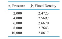
^2= & (2.486-2.4723)^2+(2.479-2.4723)^2+(2.472-2.4723)^2 \\ & +(2.558-2.5697)^2+\cdots+(2.879-2.8617)^2 \\ & +(2.858-2.8617)^2 \\ = & .005153 \end{aligned}")
^2=.289366") from equation 7.1.2.2
from equation 7.1.2.2
 and the fitted values
  . (Since in the present situation of fitting a line, the
  values,
^2=.9822=R^2")

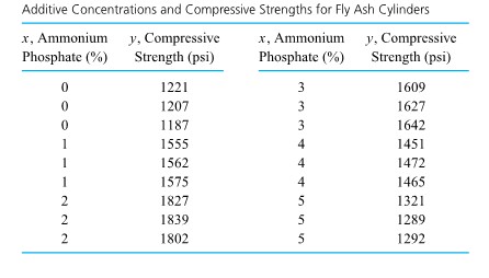

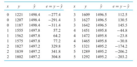
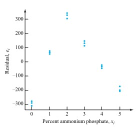

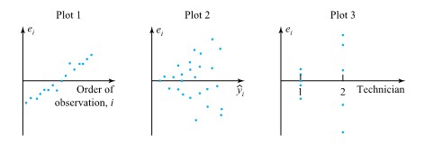
 were treated as a sample of 15 numbers and normal-plotted (using the methods we have introduced previously) to produce Figure 7.1.3.4.
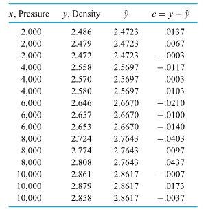
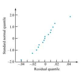

") is considered, along with inference for the average response at a given x . There follows a discussion of prediction and tolerance intervals for responses at a given setting of x . Next is an exposition of ANOVA ideas in the present situation. The section then closes with an illustration of how statistical software expedites the calculations introduced in the section.
is considered, along with inference for the average response at a given x . There follows a discussion of prediction and tolerance intervals for responses at a given setting of x . Next is an exposition of ANOVA ideas in the present situation. The section then closes with an illustration of how statistical software expedites the calculations introduced in the section. were treated as r unrestricted parameters. Turning now to the matter of inference based on data pairs
 ,\left(x_2, y_2\right), \ldots")
") exhibiting an approximately linear scatterplot, one once again proceeds by imposing a restriction on the one-way model (7.2.1.1). In words, the model assumptions will be that there are underlying normal distributions for the response y with a common variance
exhibiting an approximately linear scatterplot, one once again proceeds by imposing a restriction on the one-way model (7.2.1.1). In words, the model assumptions will be that there are underlying normal distributions for the response y with a common variance  that change linearly in
  ,
,
 . Figure 7.2.1.1 is a pictorial representation of the “constant variance, normal, linear (in x ) mean” model.


 ).
).^2=\frac{1}{n-2} \sum e^2")
 ).
). degrees of freedom and the standard error of the line-fitting model (
 , an estimated standard deviation of the response variable (
 ).
).

 estimates the level of basic background variation,
  (the pooled sample standard deviation) is another way of investigating the appropriateness of model 7.2.1.2. A
 ^2=.005153")
=.000396(\mathrm{~g} / \mathrm{cc})^2")

(.0070)^2+(3-1)(.0110)^2+\cdots+(3-1)(.0114)^2}{(3-1)+(3-1)+\cdots+(3-1)}")
^2")

 and
and 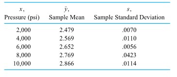
=\sigma^2\left(1-\frac{1}{n}-\frac{(x-\bar{x})^2}{\sum(x-\bar{x})^2}\right)")
^2}{\sum(x-\bar{x})^2}}}")
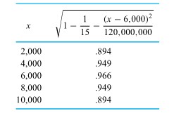
 times the appropriate entry of the second column of Table 7.2.1.3 then puts them all on equal footing, so to speak. Table 7.2.1.4 shows both the raw residuals
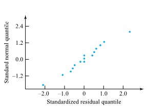

^2}")
^2}}}")
^2}}}")
 distribution. The standard arguments of Part 5 applied to expression 7.2.2.2 then show that
^2}}}")
 reference distribution. More importantly, under the simple linear re-
^2}}")
 / \mathrm{psi}")
 distribution in formula (7.2.2.5). That is, one can use endpoints

 / \mathrm{psi} \text { and } .0000526(\mathrm{~g} / \mathrm{cc}) / \mathrm{psi}")
 have mean responses differing by
  . One then simply multiplies endpoints of a confidence interval for
  \mathrm{g} / \mathrm{cc} \text { and } 2,000(.0000526) \mathrm{g} / \mathrm{cc}")

^2") is (i.e., the more spread out the
is (i.e., the more spread out the ![[a,b]](https://atu0g9ctah.execute-api.ca-central-1.amazonaws.com/latest/latex?latex=%5Ba%2Cb%5D&fg=000000&font=TeX&svg=1 "[a,b]") , taking
, taking  of them at
  and
and  produces the best possible precision for estimating the slope


^2}{\sum(x-\bar{x})^2}\right)")
^2") term appearing as a numerator in expression (7.2.3.3), the
term appearing as a numerator in expression (7.2.3.3), the ^2}{\sum(x-\bar{x})^2}}}")
^2}{\sum(x-\bar{x})^2}}}")

^2}{\sum(x-\bar{x})^2}}}")
^2}{\sum(x-\bar{x})^2}}")
") distribution. A one-sided interval is made in the usual way based on one endpoint from formula (7.2.3.7).
distribution. A one-sided interval is made in the usual way based on one endpoint from formula (7.2.3.7). \sqrt{\frac{1}{15}+\frac{(4,000-6,000)^2}{120,000,000}}=.0136 \mathrm{~g} / \mathrm{cc}")

 \sqrt{\frac{1}{15}+\frac{(5,000-6,000)^2}{120,000,000}}=.0118 \mathrm{~g} / \mathrm{cc}")

 \pm \sqrt{2 f} s_{\mathrm{LF}} \sqrt{\frac{1}{n}+\frac{(x-\bar{x})^2}{\sum(x-\bar{x})^2}}")
 probability assigned to the interval (0,
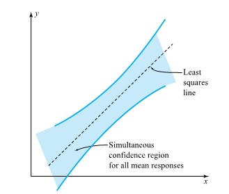
 and
and  degrees of freedom are involved in the use of formula (7.2.3.8), simultaneous limits of the form
} s_{\mathrm{LF}} \sqrt{\frac{1}{15}+\frac{(x-6,000)^2}{120,000,000}}")


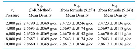
 is one additional observation, coming from the distribution of responses corresponding to a particular x ,and
 ^2}{\sum(x-\bar{x})^2}}}")
^2}{\sum(x-\bar{x})^2}}")
")
")
 is appropriately chosen (depending upon the data, p, x , and the desired confidence level).
 to
to ^2}{\sum(x-\bar{x})^2}}")
+A Q_z(\gamma) \sqrt{1+\frac{1}{2(n-2)}\left(\frac{Q_z^2(p)}{A^2}-Q_z^2(\gamma)\right)}}{1-\frac{Q_z^2(\gamma)}{2(n-2)}}")
 \sqrt{1+\frac{1}{15}+\frac{(4,000-6,000)^2}{120,000,000}}=2.5796-.0282")
^2}{120,000,000}}=.3162")
(1.645) \sqrt{1+\frac{1}{2(15-2)}\left(\frac{(1.282)^2}{(.3162)^2}-(1.645)^2\right)}}{1-\frac{(1.645)^2}{2(15-2)}}=2.149")

^2")


}")
 reference distribution, where large observed values of the test statistic constitute evidence against
  , which doesn’t depend on x . (Actually, a better interpretation of a test of hypothesis (7.2.5.2) is as a test of whether a linear term in x adds significantly to one’s ability to model the response y after accounting for an overall mean response.)
^2=.289366")
^2=.005153")

![[latex]\mathrm{H}_0: \beta_1=0](https://atu0g9ctah.execute-api.ca-central-1.amazonaws.com/latest/latex?latex=%5Blatex%5D%5Cmathrm%7BH%7D_0%3A%20%5Cbeta_1%3D0&fg=000000&font=TeX&svg=1 "[latex]\mathrm{H}_0: \beta_1=0") [/latex] is
[/latex] is![P\left[\text { an } F_{1,13} \text { random variable }>717\right]<.001](https://atu0g9ctah.execute-api.ca-central-1.amazonaws.com/latest/latex?latex=P%5Cleft%5B%5Ctext%20%7B%20an%20%7D%20F_%7B1%2C13%7D%20%5Ctext%20%7B%20random%20variable%20%7D%3E717%5Cright%5D%3C.001&fg=000000&font=TeX&svg=1 "P\left[\text { an } F_{1,13} \text { random variable }>717\right]<.001")
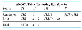
 =
=  and
and 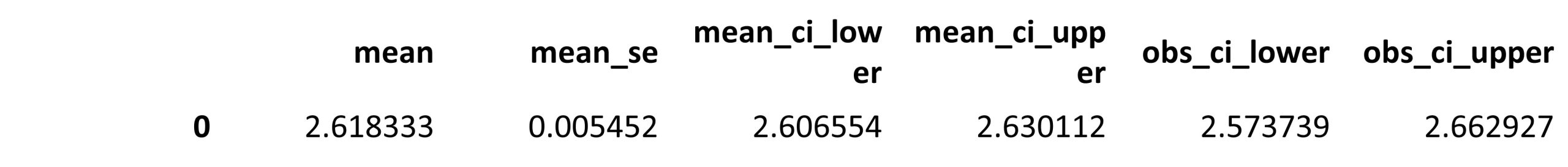
") data. Next comes the fitting of surfaces to data where a response
data. Next comes the fitting of surfaces to data where a response  . In both cases, the discussion will stress how useful
  and residual plotting are and will consider the question of choosing between possible fitted equations. Lastly, we include some additional practical cautions.

") is conceptually only slightly more difficult than the task of fitting equation (8.1.1.1). The function of
is conceptually only slightly more difficult than the task of fitting equation (8.1.1.1). The function of  variables
\right)^2 \\ & =\frac{g}{2}\left(\frac{x}{60}\right)^2+g\left(t_0-\frac{1}{60}\right)\left(\frac{x}{60}\right)+\frac{g}{2}\left(t_0-\frac{1}{60}\right)^2 \\ & =\frac{g}{7200} x^2+\frac{g}{60}\left(t_0-\frac{1}{60}\right) x+\frac{g}{2}\left(t_0-\frac{1}{60}\right)^2 \end{aligned}")
") equal to 0 , the set of normal equations is obtained for this least squares problem, generalizing the pair of equations from Part 7.1. There are
equal to 0 , the set of normal equations is obtained for this least squares problem, generalizing the pair of equations from Part 7.1. There are  . And typically, they can be solved simultaneously for a single set of values,
  , minimizing
  version of equation (8.1.1.2)
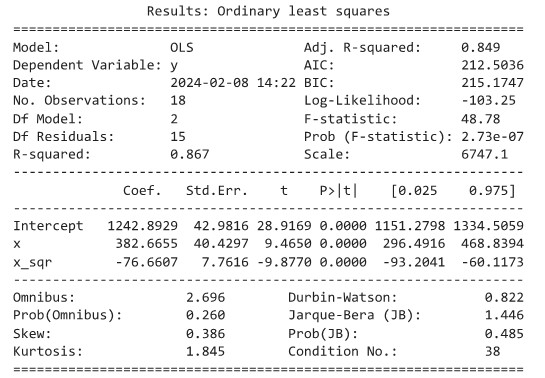


^{2}-\sum\left(y_{i}-\hat{y}_{i}\right)^{2}}{\sum\left(y_{i}-\bar{y}\right)^{2}}")

 produces
  . So
. So  of the raw variability in compressive strength is accounted for using the fitted quadratic. The sample correlation between the observed strengths
  and fitted strengths
  is
is  .
. , and
, and  for each
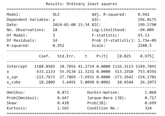

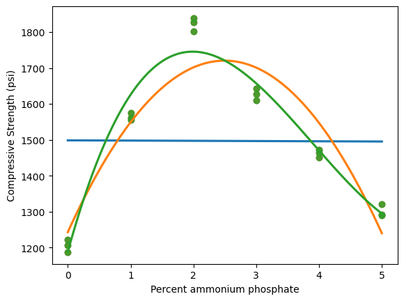
 . Unfortunately, this is where compressive strength is greatest—precisely the area of greatest practical interest.
 intervals beginning at some unknown time
  (less than

 ) will be
  . This is in fact how the value
  , quoted in Section 1.4, was obtained.
 ) with
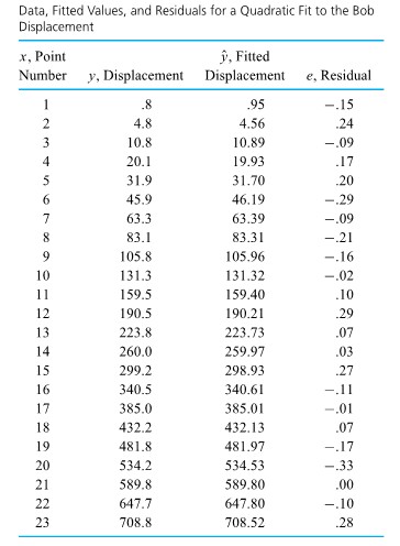

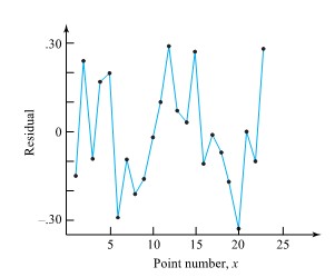
 current waveform is one matter to be addressed.
 . But having identified the region around
  ammonium phosphate. It is quite possible that a quadratic fit only to data with
  would be both adequate and helpful as a summarization of the follow-up data.
 in equation (8.1.1.2) can be replaced by any (known) functions of
 \approx \ln (\alpha)+\beta \ln (x)")
") that is linear in the parameters
that is linear in the parameters ") and
and ") . So, presented with a set of
. So, presented with a set of  (and thus
 \right)") and
and  .
.") for some function
for some function ") .
.=\ln (y)") . To illustrate its use in the present context, normal plots of both discovery times and log discovery times are given in Figure 8.1.2.2. These plots indicate that Elliot, Kibby, and Meyer could not have reasonably applied standard methods of inference to the discovery times, but they could have used the methods with log discovery times. The second normal plot is far more linear than the first.
. To illustrate its use in the present context, normal plots of both discovery times and log discovery times are given in Figure 8.1.2.2. These plots indicate that Elliot, Kibby, and Meyer could not have reasonably applied standard methods of inference to the discovery times, but they could have used the methods with log discovery times. The second normal plot is far more linear than the first.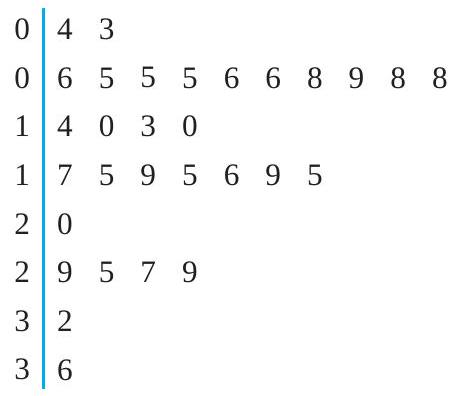

=(y-\gamma)^{\alpha}")
 , transformation (8.1.2.1) tends to lengthen the right tail of a distribution for
  , the transformation tends to shorten the right tail of a distribution for
 =\ln (y-\gamma)")
 power of the response mean, try transformation (4.34) with
  .
.") versus
versus ") and see if there is approximate linearity. If so, a slope of roughly 1 makes (1) appropriate, while a slope of
and see if there is approximate linearity. If so, a slope of roughly 1 makes (1) appropriate, while a slope of  signals what version of (2) might be helpful.
") data points are pictured in three dimensions, along with a possible fitted surface of the form (8.1.3.1). To fit a surface defined by equation (8.1.3.1) to a set of
data points are pictured in three dimensions, along with a possible fitted surface of the form (8.1.3.1). To fit a surface defined by equation (8.1.3.1) to a set of ") via least squares, the function of
via least squares, the function of =\sum_{i=1}^{n}\left(y_{i}-\hat{y}_{i}\right)^{2}=\sum_{i=1}^{n}\left(y_{i}-\left(\beta_{0}+\beta_{1} x_{1 i}+\cdots+\beta_{k} x_{k i}\right)\right)^{2}")
") .
.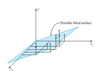
 , is the percent circulating minus 50 times 10 . The response variable,
  , and
, and 
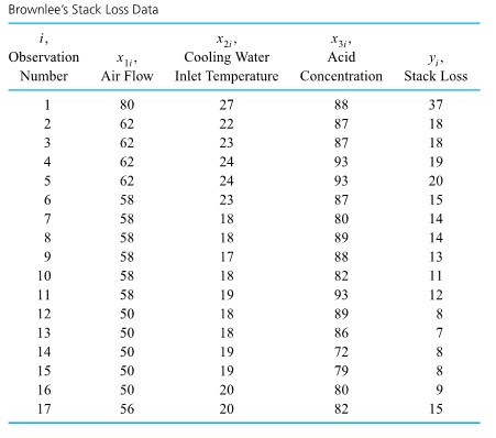

 . The coefficients in this equation can be thought of as rates of change of stack loss with respect to the individual variables
  can be interpreted as the increase in stack loss
  is positive indicates that the higher the rate at which the plant is run, the larger
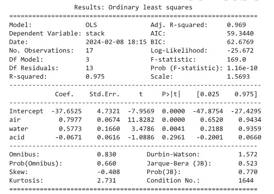
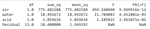
") data to “see” how an equation is fitting. About all that we can do at this point is to (1) offer the broad advice that what is wanted is the simplest equation that adequately fits the data and then (2) provide examples of how
data to “see” how an equation is fitting. About all that we can do at this point is to (1) offer the broad advice that what is wanted is the simplest equation that adequately fits the data and then (2) provide examples of how  of the raw variability in stack loss. Inclusion of
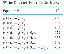
 \approx 1.5")
 the fitted rate of change in
 , and
, and  in equation (8.1.3.3) differ somewhat from the corresponding values in equation (8.1.3.2). That is, equation (8.1.3.3) was not obtained from equation
 will change depending on which
  term to the fitted equation (8.1.3.3).

 and residuals that show even less of a pattern than those for the fitted equation (8.1.3.3). In particular, the hint of curvature on the plot of residuals versus
 ![x_{3}[latex] and equation (8.1.3.4) does not.</div> </div> <div>.</div> <div> [caption id="attachment_450" align="aligncenter" width="546"]<img class="wp-image-450 size-full" src="https://ecampusontario.pressbooks.pub/app/uploads/sites/4023/2024/02/120_1.jpg" alt="" width="546" height="454" /> Figure 8.1.3.2 Plots of residuals from a two-variable equation fit to the stack loss data ( yˆ =−42.00 − .78x1 + .57x2 )[/caption] . Equation (8.1.3.4) is somewhat more complicated than equation (8.1.3.3). But because it still really only involves two different input [latex]x](https://atu0g9ctah.execute-api.ca-central-1.amazonaws.com/latest/latex?latex=x_%7B3%7D%5Blatex%5D%20and%20equation%20%288.1.3.4%29%20does%20not.%3C%2Fdiv%3E%20%20%3C%2Fdiv%3E%20%20%3Cdiv%3E.%3C%2Fdiv%3E%20%20%3Cdiv%3E%20%20%20%20%5Bcaption%20id%3D%22attachment_450%22%20align%3D%22aligncenter%22%20width%3D%22546%22%5D%3Cimg%20class%3D%22wp-image-450%20size-full%22%20src%3D%22https%3A%2F%2Fecampusontario.pressbooks.pub%2Fapp%2Fuploads%2Fsites%2F4023%2F2024%2F02%2F120_1.jpg%22%20alt%3D%22%22%20width%3D%22546%22%20height%3D%22454%22%20%2F%3E%20Figure%208.1.3.2%20Plots%20of%20residuals%20from%20a%20two-variable%20equation%20%EF%AC%81t%20to%20the%20stack%20loss%20data%20%28%20y%CB%86%20%3D%E2%88%9242.00%20%E2%88%92%20.78x1%20%2B%20.57x2%20%29%5B%2Fcaption%5D%20%20%20%20.%20%20%20%20Equation%20%288.1.3.4%29%20is%20somewhat%20more%20complicated%20than%20equation%20%288.1.3.3%29.%20But%20because%20it%20still%20really%20only%20involves%20two%20different%20input%20%5Blatex%5Dx&fg=000000&font=TeX&svg=1 "x_{3}[latex] and equation (8.1.3.4) does not.</div> </div> <div>.</div> <div> [caption id="attachment_450" align="aligncenter" width="546"]<img class="wp-image-450 size-full" src="https://ecampusontario.pressbooks.pub/app/uploads/sites/4023/2024/02/120_1.jpg" alt="" width="546" height="454" /> Figure 8.1.3.2 Plots of residuals from a two-variable equation fit to the stack loss data ( yˆ =−42.00 − .78x1 + .57x2 )[/caption] . Equation (8.1.3.4) is somewhat more complicated than equation (8.1.3.3). But because it still really only involves two different input [latex]x") 's and also eliminates the slight pattern seen on the plot of residuals for equation (8.1.3.3) versus
's and also eliminates the slight pattern seen on the plot of residuals for equation (8.1.3.3) versus 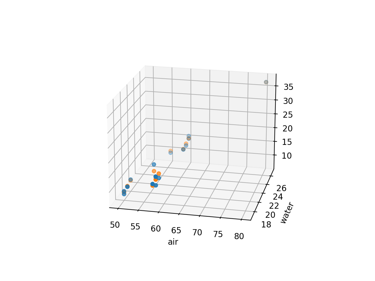
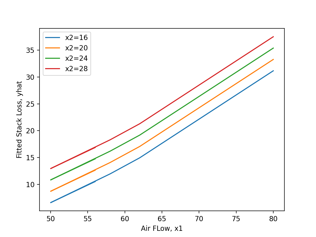
 canard placement in inches above the plane defined by the main wing
 tail placement in inches above the plane defined by the main wing


 and the fitted relationship
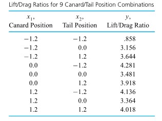
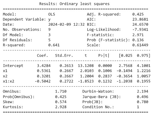
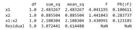

 products were created and
 ") surface would be parallel for various
surface would be parallel for various 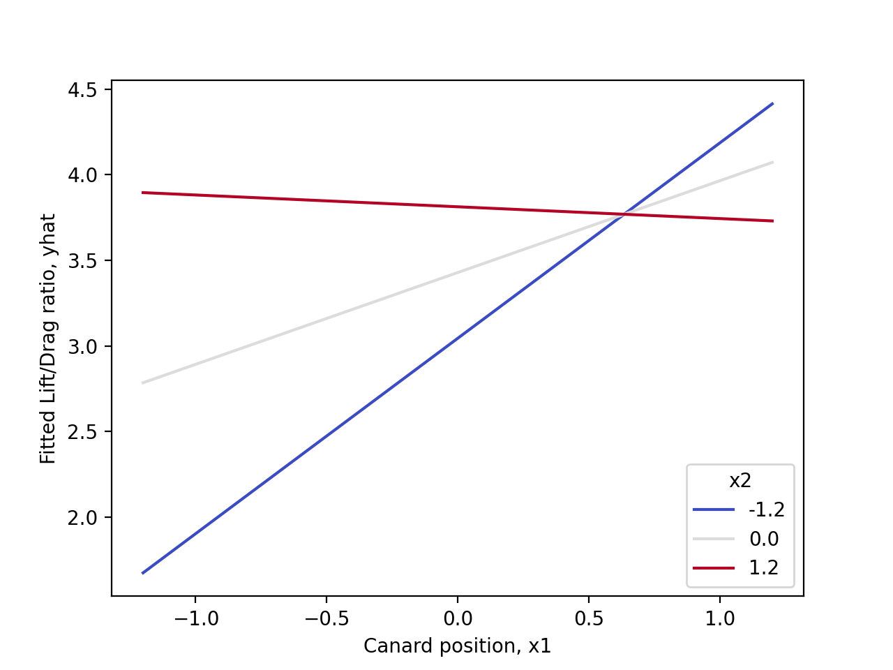

 and generally random-looking residuals. It can be verified by plotting
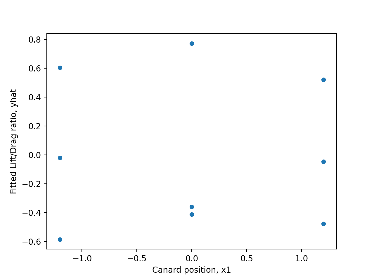
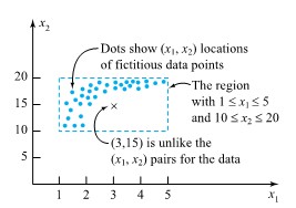
") pairs for the data in Table 8.1.3. It shows that by most qualitative standards, observation 1 in Table 8.1.3. is unusual or outlying.
pairs for the data in Table 8.1.3. It shows that by most qualitative standards, observation 1 in Table 8.1.3. is unusual or outlying.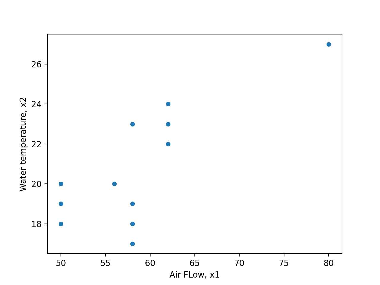

 are obtained. Using equation (8.1.61) as a description of stack loss and limiting attention to
  version of a polynomial through each of these points. But in most physical problems, such a curve would do a much worse job of predicting
  codes for each category except the referent group (which is omitted). Several examples of categorical variables that can be represented in multiple regression with dummy variables include:
 , control
 ") for the “dummied” group. This is illustrated in Figure 8.2.1.1. In this illustration, the value of
for the “dummied” group. This is illustrated in Figure 8.2.1.1. In this illustration, the value of  (a continuous variable) and
  (a dummy variable). When
  , the value of
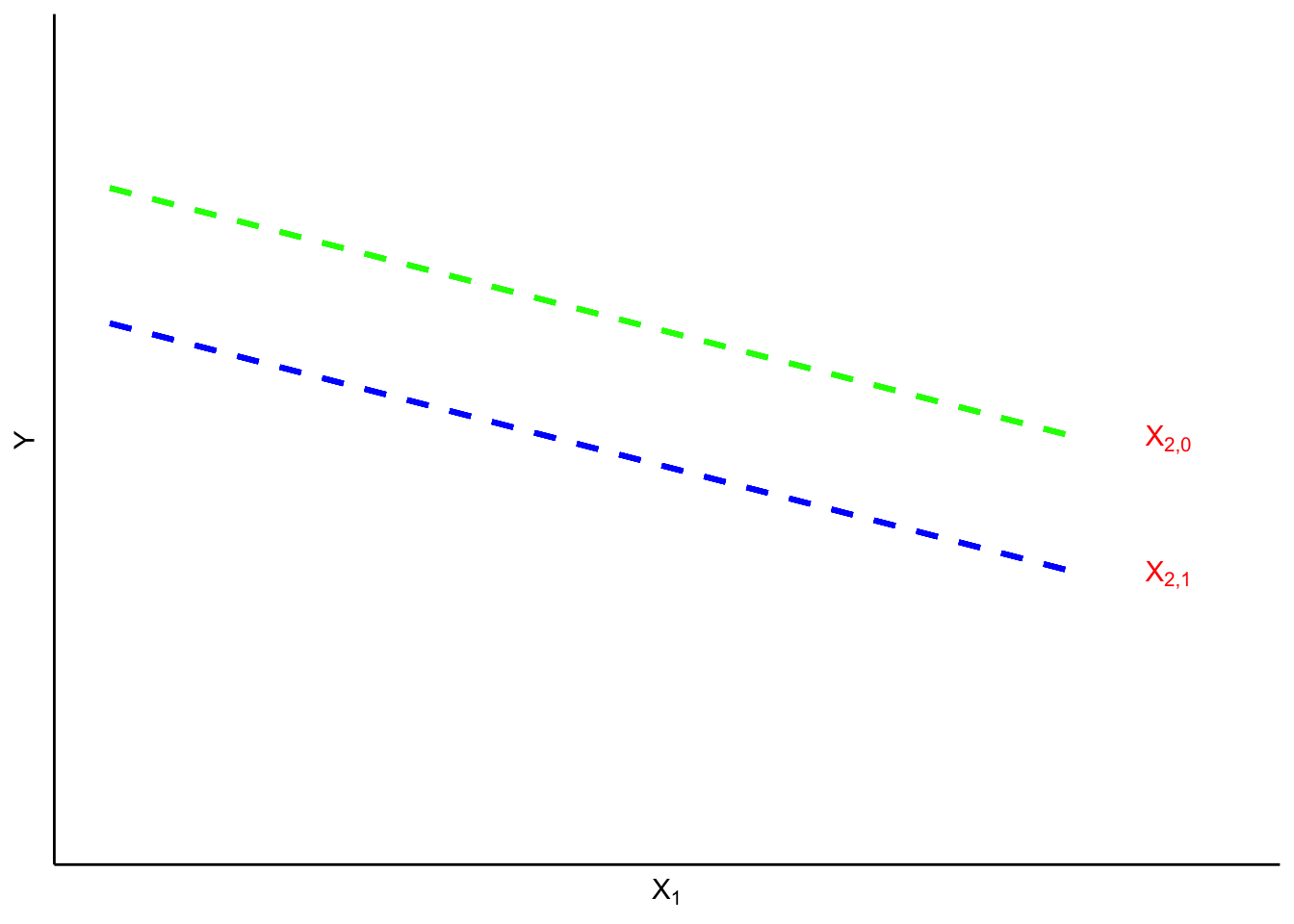
 .
. .
. women,
  men
men ") could be interacted with ideology
could be interacted with ideology  strong liberal,
  strong conservative) to predict levels of perceived risk of climate change (
  no risk,
  extreme risk). If your hypothesized interaction was correct, you would observe the kind of pattern as shown in Figure 8.2.1.2.
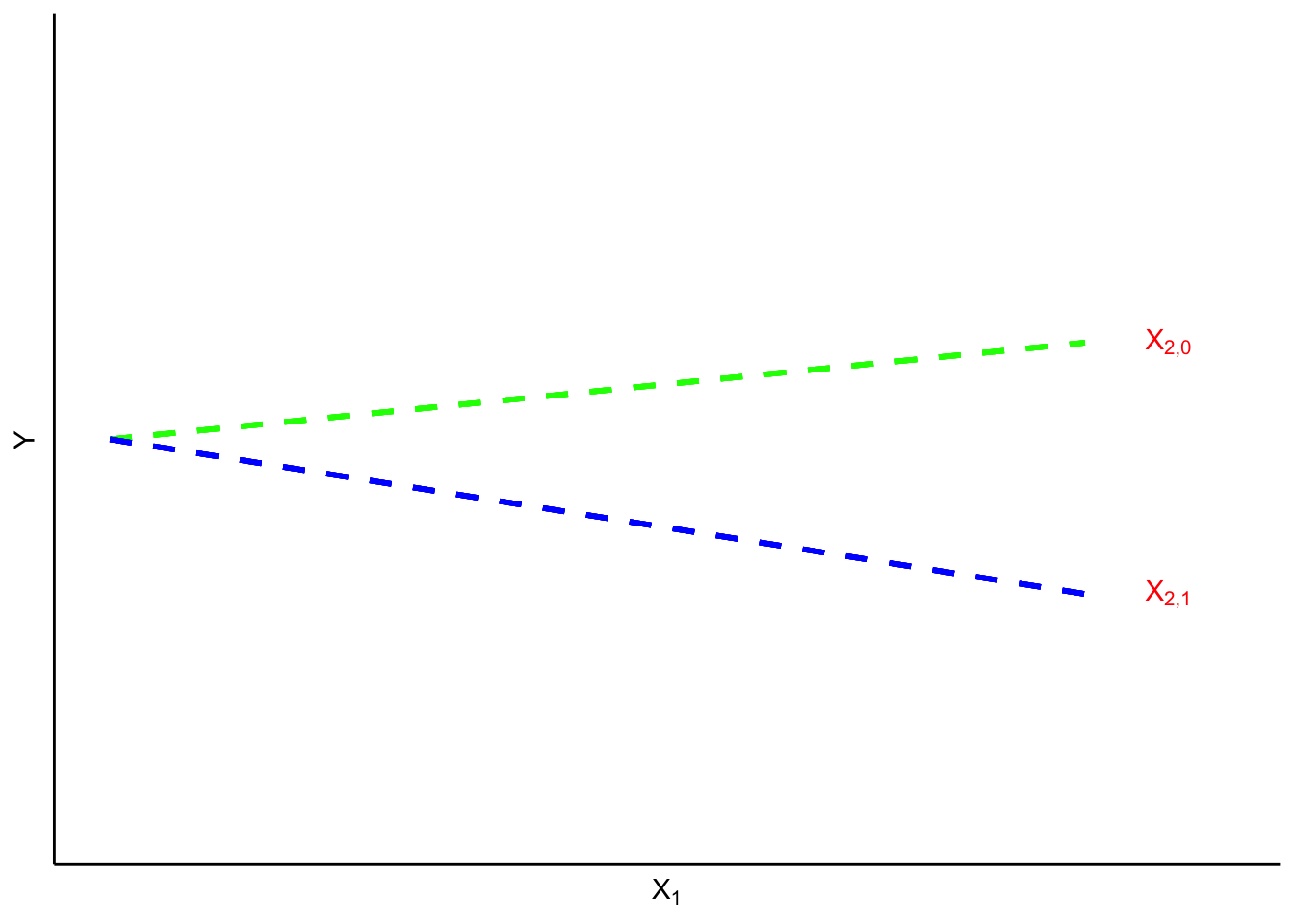
 . Using matrix notation, the same equation can be expressed in a more compact and (believe it or not!) intuitive form:
  .
. . In the following example,
 ![A_{m, n}=\left[\begin{array}{cccc}a_{1,1} & a_{1,2} & \cdots & a_{1, n} \\ a_{2,1} & a_{2,2} & \cdots & a_{2, n} \\ \vdots & \vdots & \ddots & \vdots \\ a_{m, 1} & a_{m, 2} & \cdots & a_{m, n}\end{array}\right]](https://atu0g9ctah.execute-api.ca-central-1.amazonaws.com/latest/latex?latex=A_%7Bm%2C%20n%7D%3D%5Cleft%5B%5Cbegin%7Barray%7D%7Bcccc%7Da_%7B1%2C1%7D%20%26%20a_%7B1%2C2%7D%20%26%20%5Ccdots%20%26%20a_%7B1%2C%20n%7D%20%5C%5C%20a_%7B2%2C1%7D%20%26%20a_%7B2%2C2%7D%20%26%20%5Ccdots%20%26%20a_%7B2%2C%20n%7D%20%5C%5C%20%5Cvdots%20%26%20%5Cvdots%20%26%20%5Cddots%20%26%20%5Cvdots%20%5C%5C%20a_%7Bm%2C%201%7D%20%26%20a_%7Bm%2C%202%7D%20%26%20%5Ccdots%20%26%20a_%7Bm%2C%20n%7D%5Cend%7Barray%7D%5Cright%5D&fg=000000&font=TeX&svg=1 "A_{m, n}=\left[\begin{array}{cccc}a_{1,1} & a_{1,2} & \cdots & a_{1, n} \\ a_{2,1} & a_{2,2} & \cdots & a_{2, n} \\ \vdots & \vdots & \ddots & \vdots \\ a_{m, 1} & a_{m, 2} & \cdots & a_{m, n}\end{array}\right]")
![A=\left[\begin{array}{ccc}10 & 5 & 8 \\ -12 & 1 & 0\end{array}\right]](https://atu0g9ctah.execute-api.ca-central-1.amazonaws.com/latest/latex?latex=A%3D%5Cleft%5B%5Cbegin%7Barray%7D%7Bccc%7D10%20%26%205%20%26%208%20%5C%5C%20-12%20%26%201%20%26%200%5Cend%7Barray%7D%5Cright%5D&fg=000000&font=TeX&svg=1 "A=\left[\begin{array}{ccc}10 & 5 & 8 \\ -12 & 1 & 0\end{array}\right]")
 and
and  .
.![A=\left[\begin{array}{c}6 \\ -1 \\ 8 \\ 11\end{array}\right]](https://atu0g9ctah.execute-api.ca-central-1.amazonaws.com/latest/latex?latex=A%3D%5Cleft%5B%5Cbegin%7Barray%7D%7Bc%7D6%20%5C%5C%20-1%20%5C%5C%208%20%5C%5C%2011%5Cend%7Barray%7D%5Cright%5D&fg=000000&font=TeX&svg=1 "A=\left[\begin{array}{c}6 \\ -1 \\ 8 \\ 11\end{array}\right]")
![A=\left[\begin{array}{llll}1 & 2 & 8 & 7\end{array}\right]](https://atu0g9ctah.execute-api.ca-central-1.amazonaws.com/latest/latex?latex=A%3D%5Cleft%5B%5Cbegin%7Barray%7D%7Bllll%7D1%20%26%202%20%26%208%20%26%207%5Cend%7Barray%7D%5Cright%5D&fg=000000&font=TeX&svg=1 "A=\left[\begin{array}{llll}1 & 2 & 8 & 7\end{array}\right]")
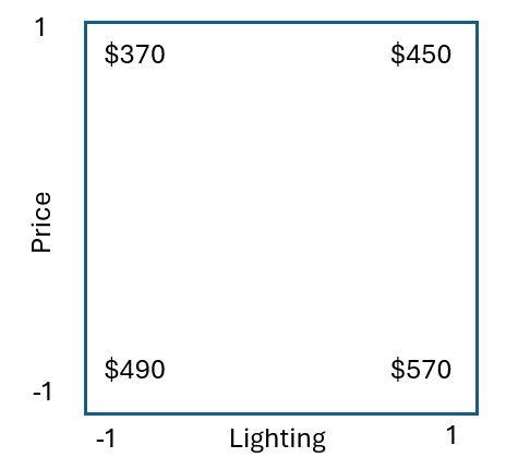
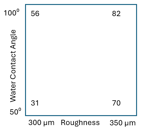
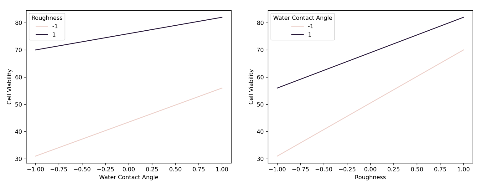
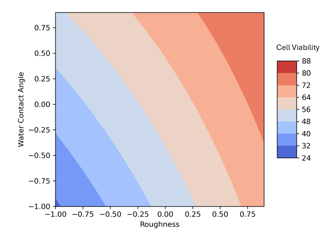

 Surface Roughness and
  Water Contact Angle):
} \\ 1 & {R+} &{W-} &{(R+W-)} \\ 1 & {R-} & {W+} &{(R-W+)} \\ 1 & {R+} & {W+} &{(R+W+)}\\\end{bmatrix}\begin{bmatrix} b_0 \\ b_R \\ b_W \\ b_{RW}\\\end{bmatrix} +\begin{bmatrix} e_0 \\ e_R \\ e_W \\ e_{RW}\\\end{bmatrix}")

}") has only non-zero values on the diagonal. Therefore:
has only non-zero values on the diagonal. Therefore:^-1(X^Ty)}")


^-1(X^Ty)}=\begin{bmatrix} (1/4) & 0 & 0 & 0 \\ 0 & (1/4) &0 &0 \\ 0 & 0 & (1/4) &0 \\ 0 & 0 & 0 &(1/4)\\\end{bmatrix}\begin{bmatrix} 239 \\ 65 \\ 37 \\ -13 \\\end{bmatrix}=\begin{bmatrix} 59.75\\ 16.25 \\ 9.25 \\ -3.25 \\\end{bmatrix}")
 , can be interpreted the same manner as before. For example, a 1 unit increase in roughness corresponds to a 16.25 a.u. increase in cell viability. This method also explains why we had to divide by 2 a second time earlier since this coefficient represents the effect of changing surface roughness from 0 to 1 or from 325 to 350 µm. The same is true for water contact angle as well. Finally, the interaction term decreases cell viability by 3.25 units if both surface roughness and water contact angle are at the same level (both high or both low).
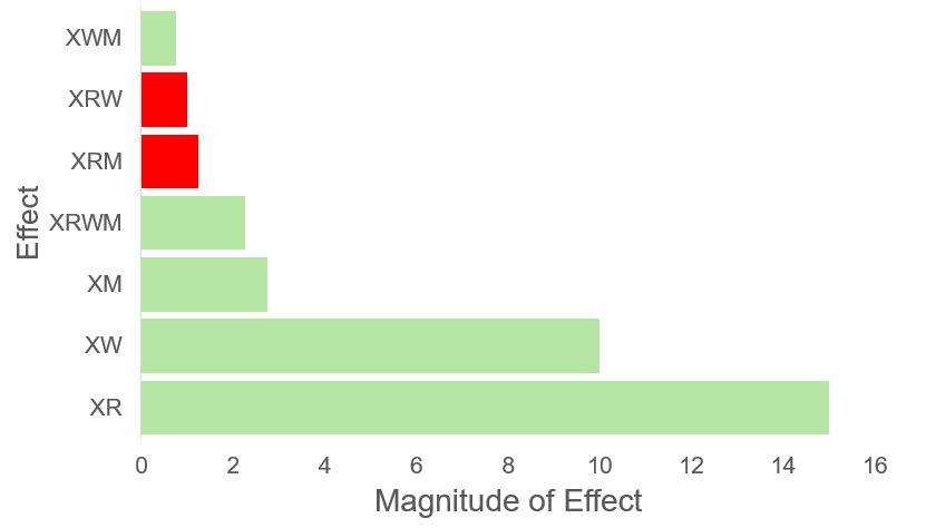
 Material Coefficient):

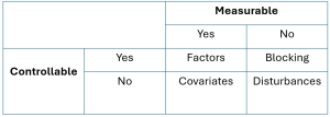
 ABC interaction effect + disturbance.
 ) will now be confounded with an interaction term.


 is confounded with the interaction of
  , since the model coefficient is the sum of these two effects. From this we can state that
  is an alias for
  , that
  is an alias for
  and that the intercept is aliased with the 3-factor interaction


 . Factors
  . This is called the generating relation.
 is a column of ones.

 . Take the generating relation and multiply both sides by Through some algebra we can also establish the defining relation of
  by the following equation:
 which tells us that
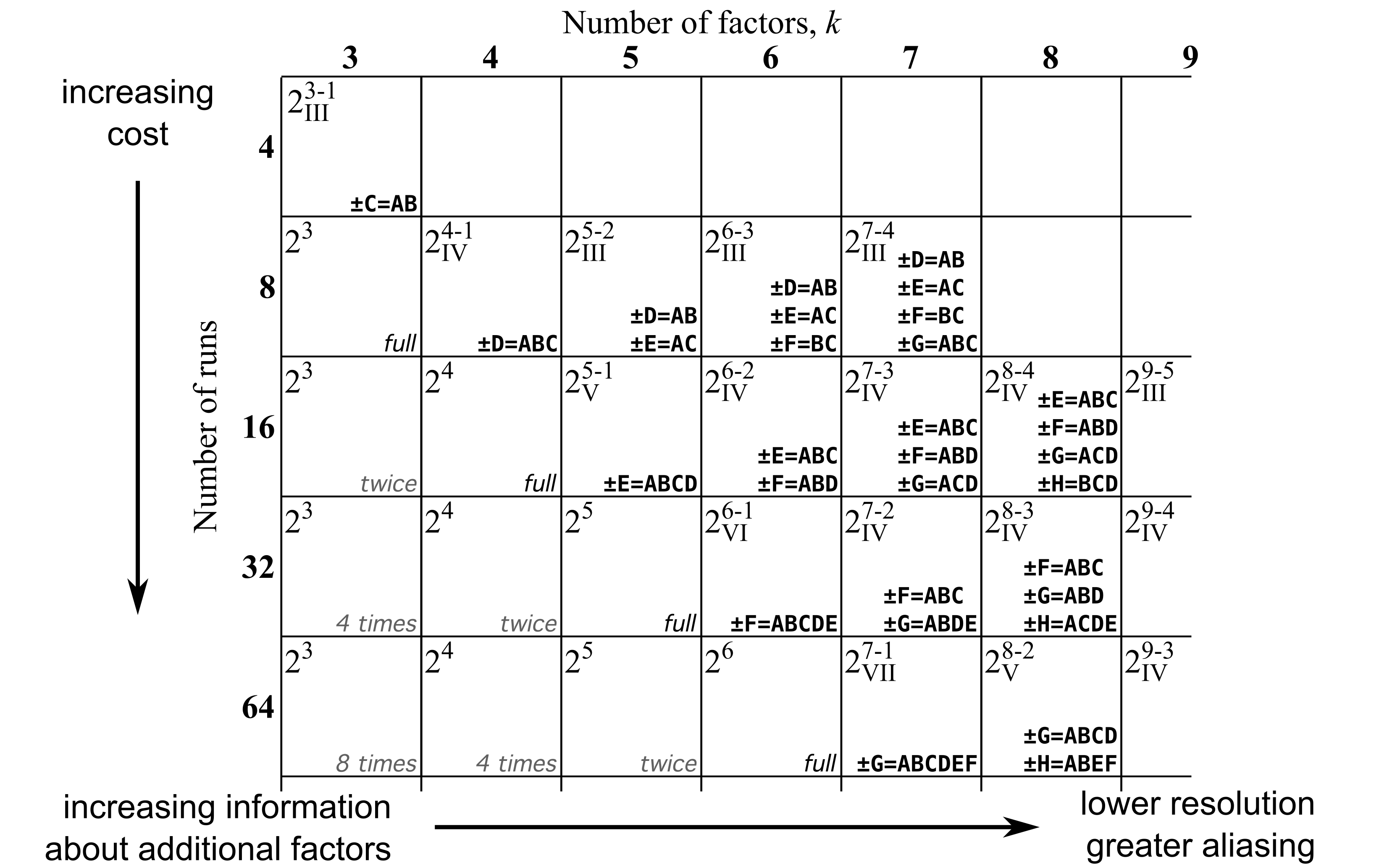
 . Here the roman numerals
  indicate the level of resolution for the design. This number is equivalent to the number of factors present in the defining relation. Since


![</span>\begin{split}\hat{y} &= b_0 + b_T x_T + b_S x_S + b_{TS} x_T x_S \\ \hat{y} &= 389.8 + 55 x_T + 134 x_S - 3.50 x_T x_S\end{split}</div> where <span class="math notranslate nohighlight">[latex]x_T = \dfrac{x_{T,\text{actual}} - \text{center}_T}{\Delta_T/2}](https://atu0g9ctah.execute-api.ca-central-1.amazonaws.com/latest/latex?latex=%3C%2Fspan%3E%5Cbegin%7Bsplit%7D%5Chat%7By%7D%20%26%3D%20b_0%20%2B%20b_T%20x_T%20%2B%20b_S%20x_S%20%2B%20b_%7BTS%7D%20x_T%20x_S%20%5C%5C%20%20%5Chat%7By%7D%20%26%3D%20389.8%20%2B%2055%20x_T%20%2B%20134%20x_S%20-%203.50%20x_T%20x_S%5Cend%7Bsplit%7D%3C%2Fdiv%3E%20%20where%20%3Cspan%20class%3D%22math%20notranslate%20nohighlight%22%3E%5Blatex%5Dx_T%20%3D%20%5Cdfrac%7Bx_%7BT%2C%5Ctext%7Bactual%7D%7D%20-%20%5Ctext%7Bcenter%7D_T%7D%7B%5CDelta_T%2F2%7D&fg=000000&font=TeX&svg=1 "</span>\begin{split}\hat{y} &= b_0 + b_T x_T + b_S x_S + b_{TS} x_T x_S \\ \hat{y} &= 389.8 + 55 x_T + 134 x_S - 3.50 x_T x_S\end{split}</div> where <span class="math notranslate nohighlight">[latex]x_T = \dfrac{x_{T,\text{actual}} - \text{center}_T}{\Delta_T/2}")


K")
g/L")


 = (0,0)")


 .
.
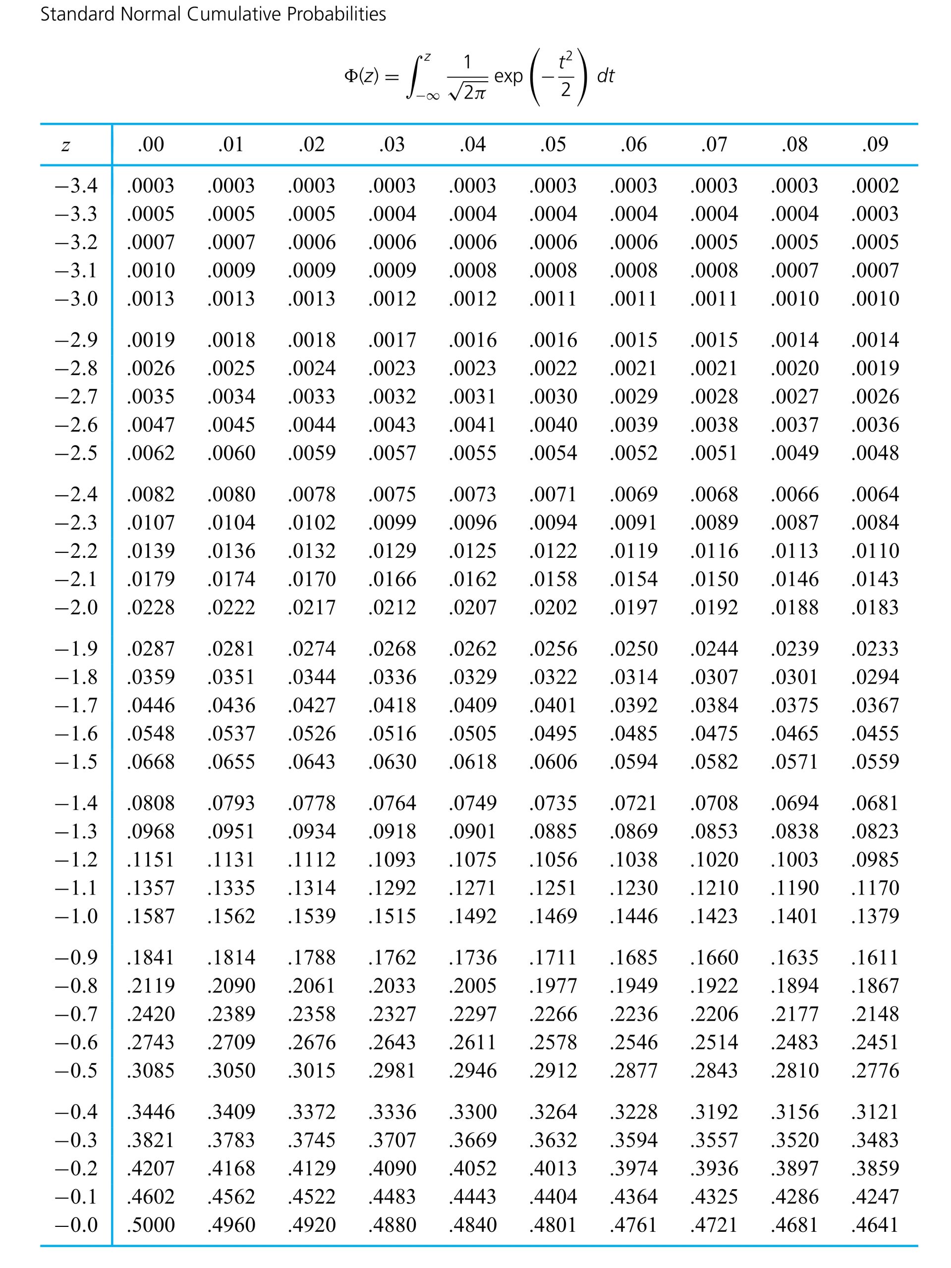
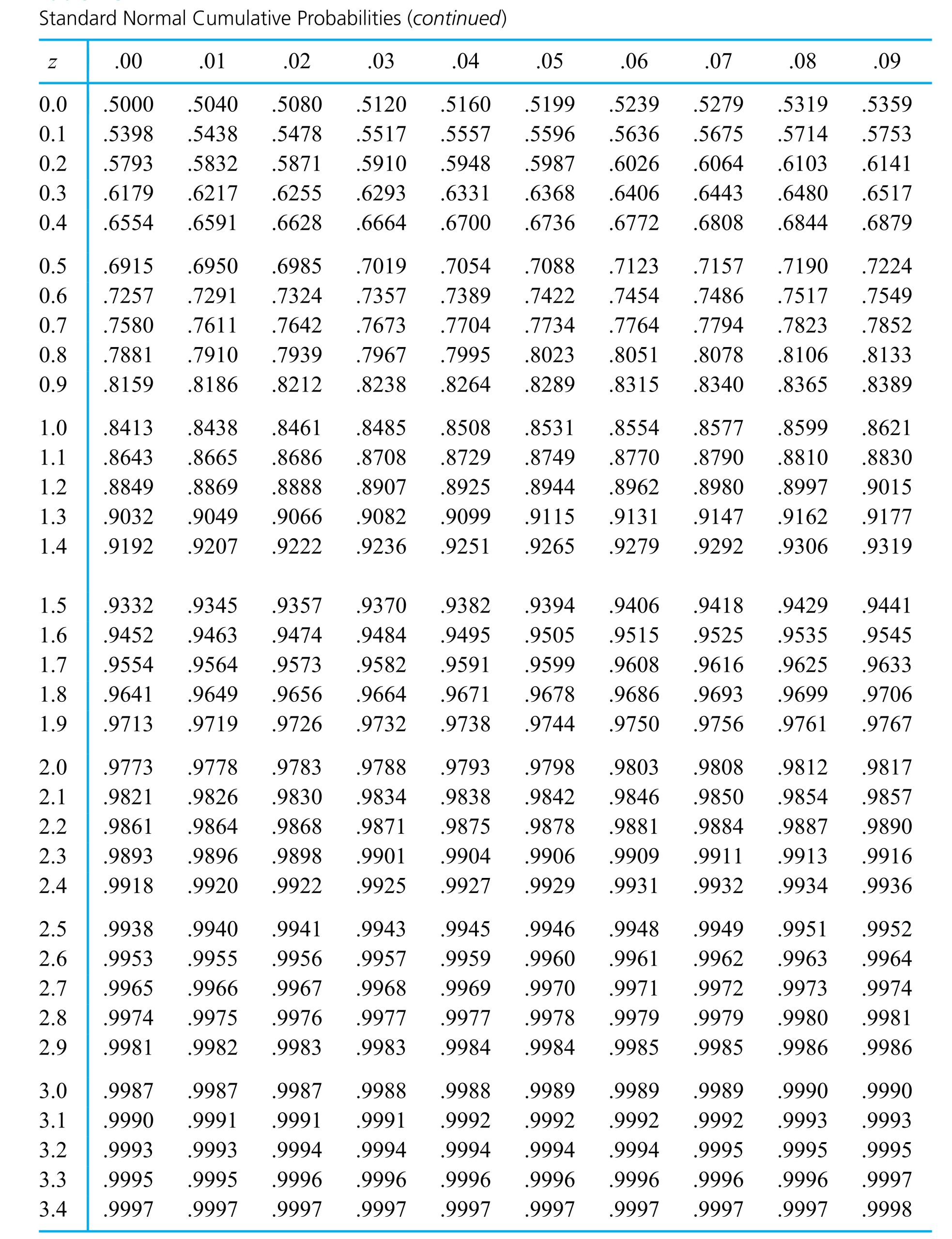

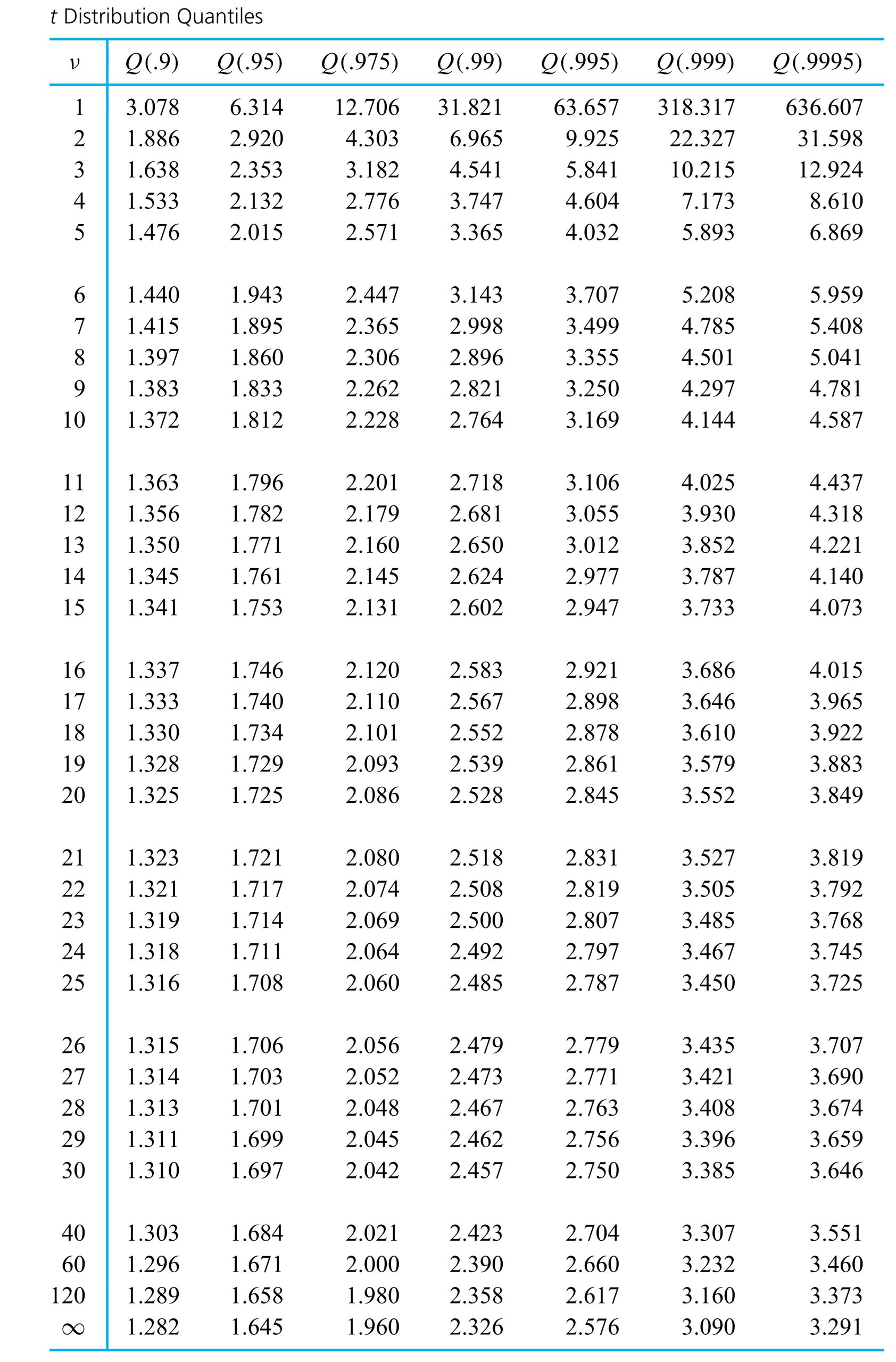
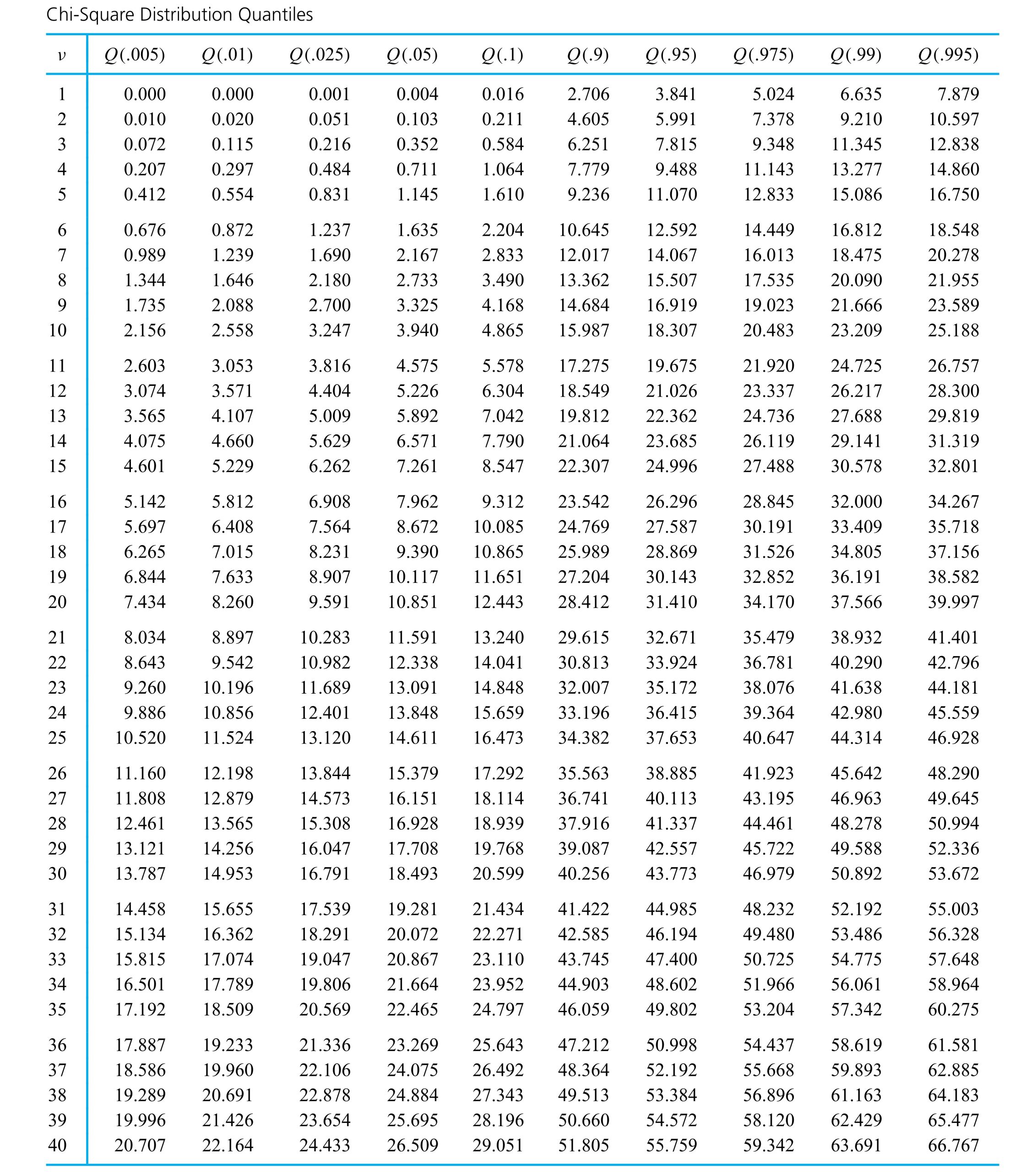
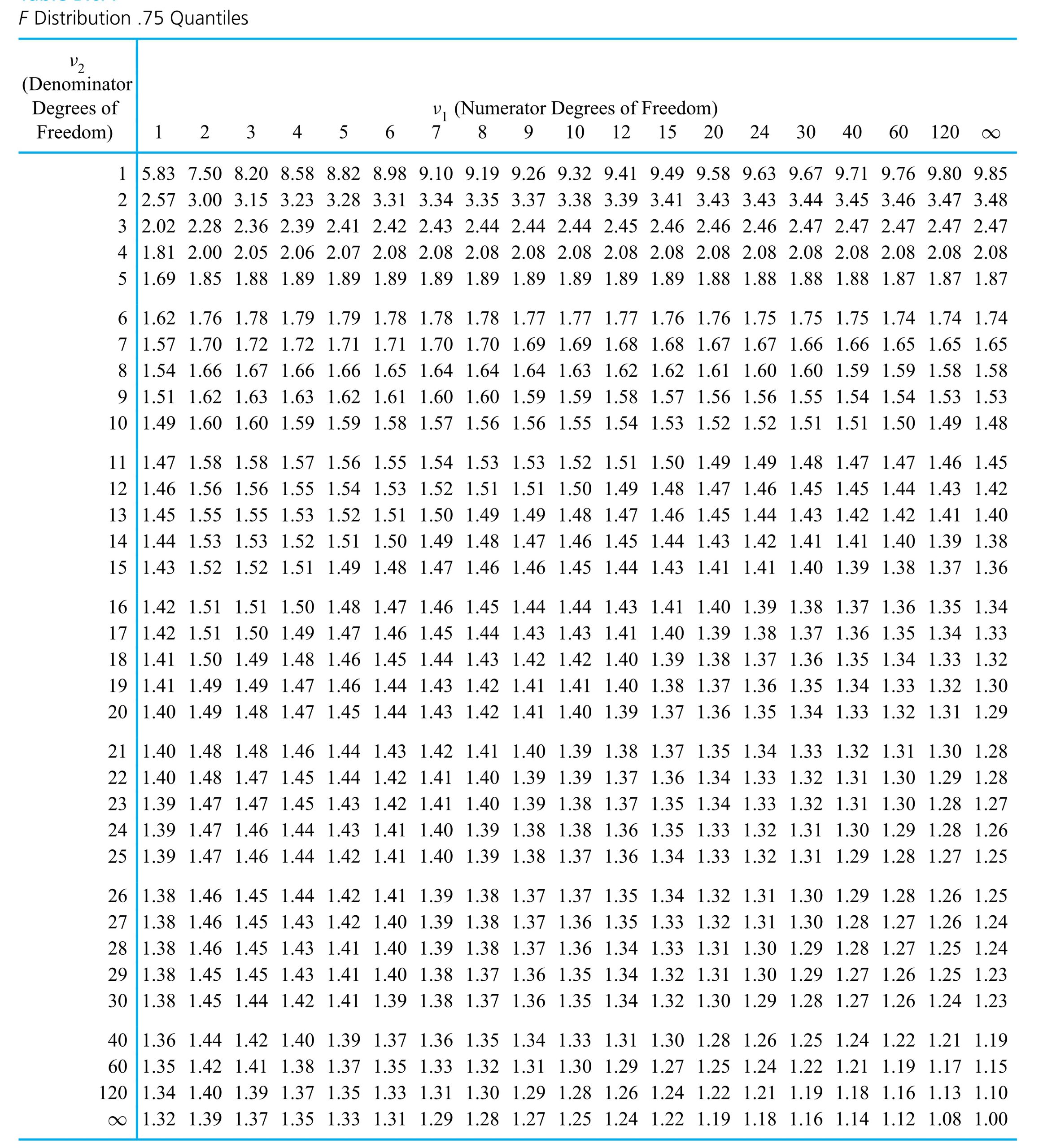

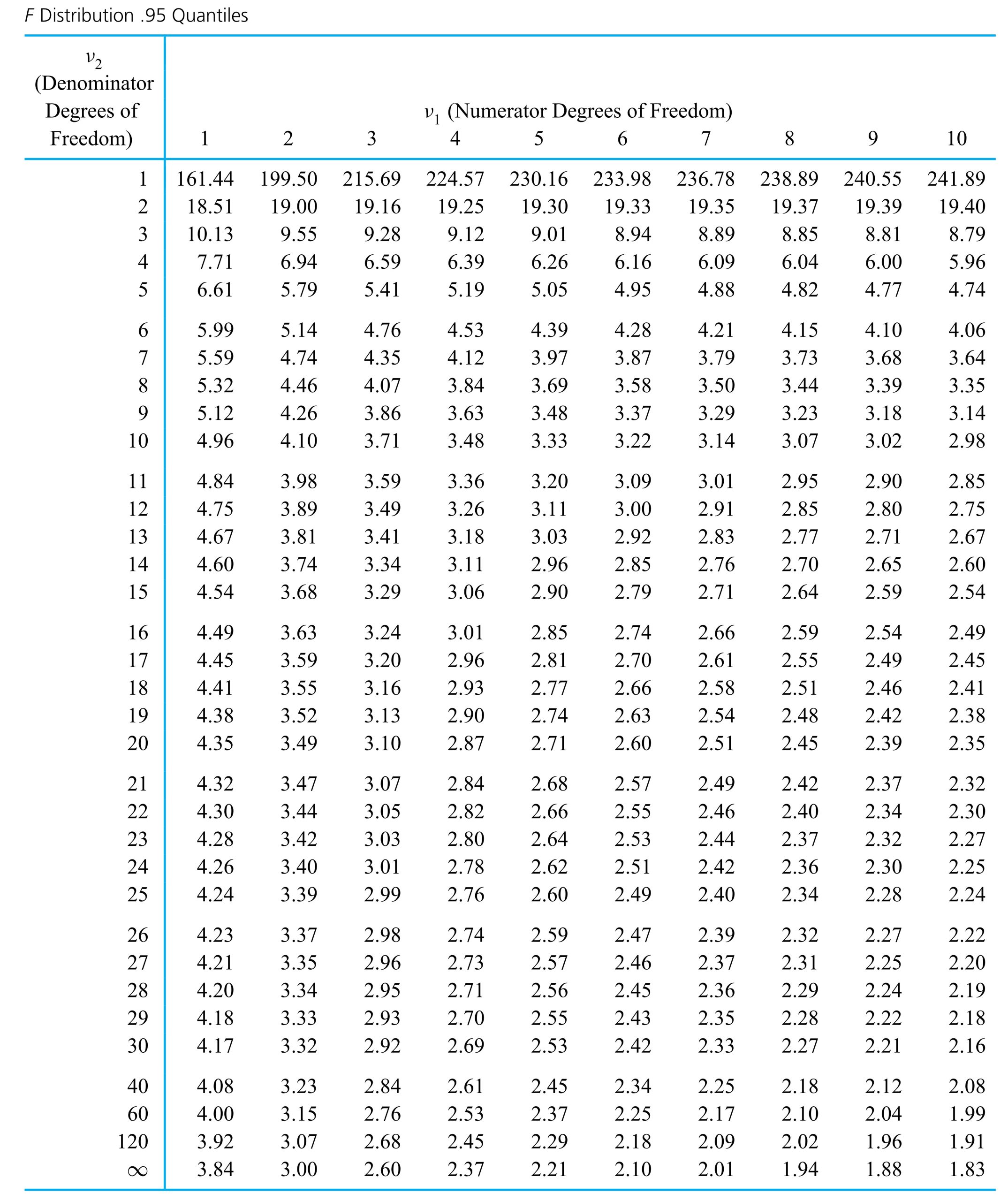
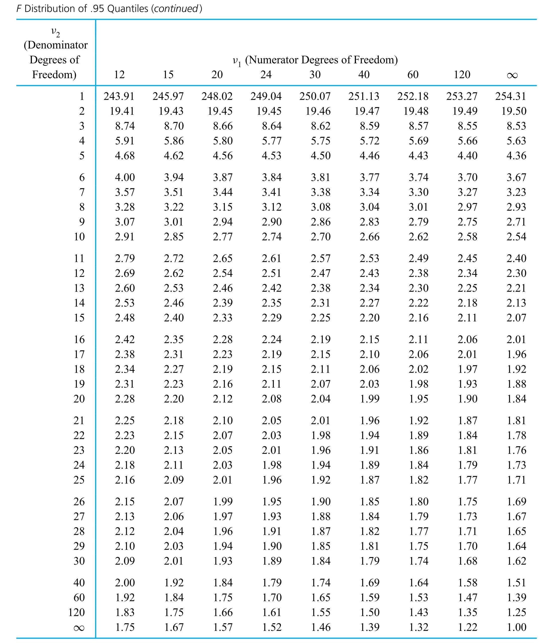
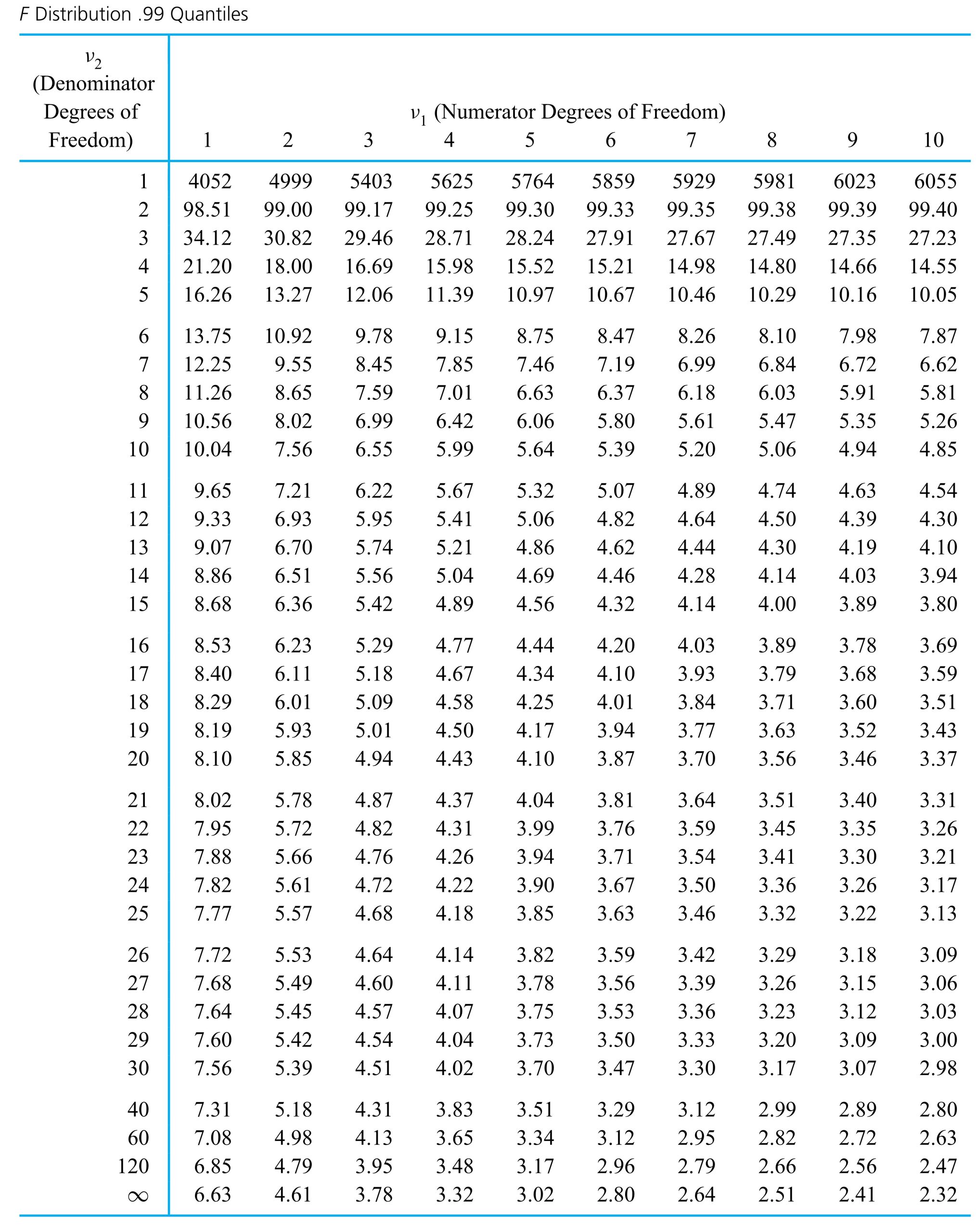
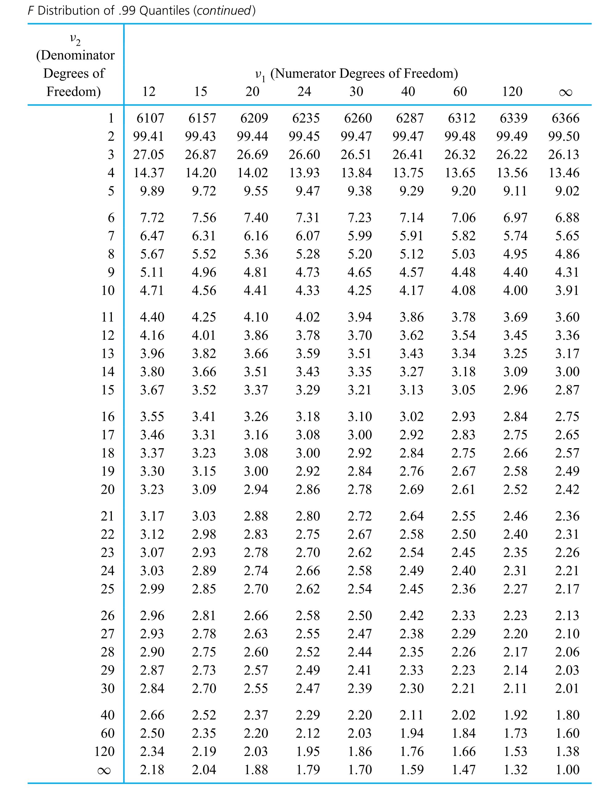
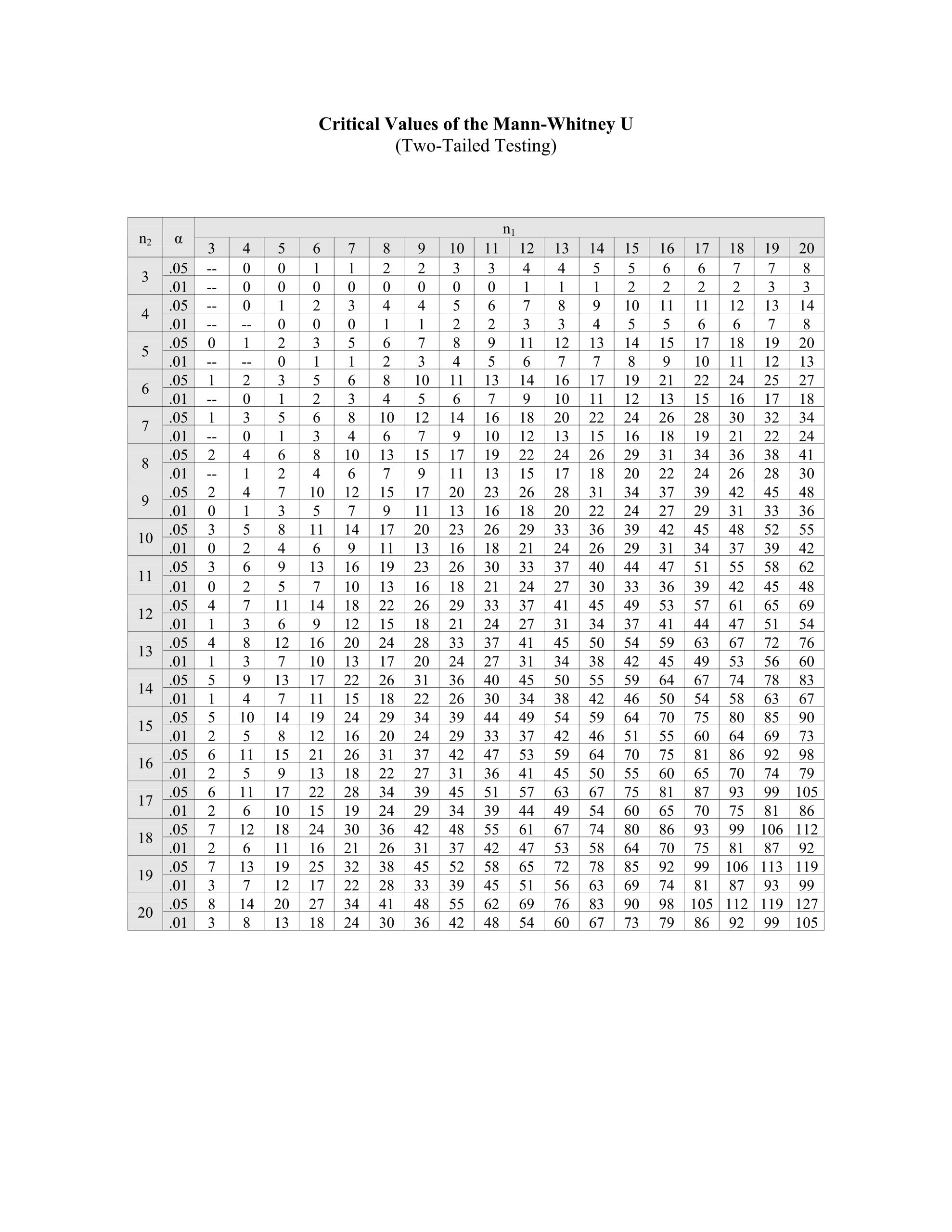
