In earlier chapters, we looked at the effects of government policies used to protect domestic producers from import competition. Sometimes, governments support their domestic producers by helping them to increase their sales in foreign markets. Two strategies that governments and their domestic producers use to raise foreign sales are dumping and export subsidies. We will examine the economic effects of these strategies on the exporting country, on the importing country, and on the world as a whole. Many countries consider dumping and export subsidies to be unfair trade and often retaliate against their use. Indeed, the WTO outlaws export subsidies, allows antidumping and countervailing duties to be applied, and has a mechanism to resolve disputes stemming from the use of these practices.
Dumping
Dumping is the selling of products in foreign markets at prices that are below fair market value. One interpretation of fair market value is the price paid by similar buyers in the producer’s domestic market or in a third-country market if no domestic market exists for the product. Under this price-based definition, dumping occurs whenever a producer sells the product in a foreign market at a price below that in the reference market, after allowing for transportation and other costs. On this basis, dumping is international price discrimination, i.e., selling the same product to different buyers at different prices. Another interpretation of “fair market value” is average total cost of production, including an element for profit and overhead expenses. Dumping, according to this view, involves selling in foreign markets at a price less than the cost of production.
There are different types of dumping, namely, predatory dumping, sporadic dumping, and persistent dumping. Predatory dumping refers to the situation in which a firm initially charges a low price in the foreign market with the aim of getting rid of the competition. Once rival firms are driven out, the firm uses its now dominant market position to raise prices and its profits. For this strategy to be successful, the firm must feel confident that the new price will be high enough over a relatively long period to compensate for any losses incurred when the low initial price was in effect. Although predatory dumping is possible, there has been no real evidence to support its existence (Carbaugh, 2015; Pugel, 2020).
Sporadic dumping occurs when a firm disposes of excess inventories by selling in a foreign market at a lower price than in the domestic market (Carbaugh, 2015). Excess inventories may result from a recession in the domestic economy, seasonal increases in production, or improper planning. A firm may lower its prices during a recession to contain any decline in sales. If the domestic market price falls below the average total cost of production, the firm may continue its sales once the price it charges covers its variable cost. If any of these sales are made abroad, then this would be dumping. Sporadic dumping can be disruptive to competing firms in importing countries.
Persistent dumping occurs when a firm uses international price discrimination to increase its profits. For international price discrimination to be effective, demand conditions differ in the foreign and domestic markets, and the firm must be able to separate the domestic market from the foreign market. Once demand elasticities in the two markets differ and reselling across markets is hard to accomplish, this type of dumping can persist. In practice, because of high transportation costs and the existence of trade restrictions, it is relatively easy to keep international markets separate.
Persistent dumping is illustrated in Figure 7.1. The analysis shows that international price discrimination raises sales and profits. We assume that marginal cost is constant and identical for product sales in both domestic and foreign markets. We assume that demand for the firm’s product in the domestic market is inelastic while demand in the foreign market is elastic. This means that consumers in the domestic market are unlikely to significantly reduce how much they buy in response to a price increase. In contrast, foreign consumers are very likely to cut their purchases a lot if the firm raises the price.
In both markets, the firm chooses its profit-maximizing quantity by equating marginal revenue and marginal cost and charging the highest price consistent with demand conditions. The firm attains a higher price in the domestic market, where demand is inelastic, and a lower price in the foreign market, where demand is more elastic. Since marginal and average production costs are the same for both markets, we see that the firm makes a larger profit domestically than abroad. Moreover, we see that the firm increases its profits by extending sales to the foreign market. Once the firm can prevent reselling back into the domestic market, higher sales and profit levels can be sustained.
The Economic Effects of Dumping in a Small Importing Country
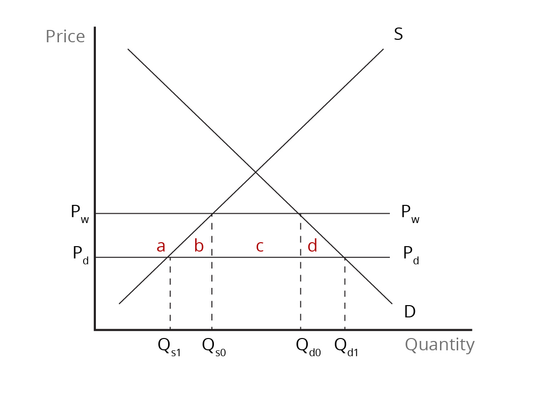
A small importing country benefits from dumping, which reduces the product price in the importing country below the world price. This means that consumer surplus in the importing country increases as consumers are able to buy a larger quantity of the product at a lower price. Meanwhile, producer surplus falls, as domestic firms now sell less at a lower price in the face of increased import competition. (See Figure 7.2). Overall, the country benefits as the increase in consumer surplus exceeds the reduction in producer surplus. This outcome is especially true for persistent dumping. However, it is unlikely to be true for predatory dumping. This is because the monopoly power that results from predatory dumping leads to reduced product availability and higher prices in the import market.
As indicated previously, many countries view dumping as an unfair trading practice that harms their domestic producers. WTO rules allow affected countries to retaliate against dumping. If there is evidence that dumping has taken place and has materially injured domestic producers, a national government can impose an anti-dumping duty to offset any unfair advantage that foreign producers have in the importing-country market and “level the playing field.” An anti-dumping duty is an additional tariff equal to the difference between the actual export price and the fair market value.
Countries have increasingly resorted to the use of antidumping laws to protect domestic producers against import competition. This is at least partly motivated by the reduction in import tariffs that has been achieved under the GATT/WTO. The protection that domestic producers get from charges of dumping is significant – average anti-dumping duties imposed against foreign exporters, on average, have been high. For example, average anti-dumping duties in Canada and the United States were in the 80-90 percent rage for the 2002–04 period (Pugel, 2020). Moreover, import-competing firms often use the threat of dumping complaints to get foreign exporters to raise their prices or reduce their exports.
Up until about 1990, a few advanced countries – the United States, Australia, the European Union and Canada – accounted for over 90% of all anti-dumping cases (Pugel, 2020, p.228). More recently, developing countries – including India, Brazil, Argentina, Turkey, Indonesia, Pakistan, and China — have increasingly filed antidumping cases. The products most involved in anti-dumping cases include steel, other metals, chemicals, plastics and rubber products, and textiles and apparel. The countries whose exports have been most frequently charged with dumping include South Korea, China, Thailand, India, and the United States (Pugel, 2020, p. 228).
Export Subsidies
National governments sometimes support their domestic producers with export subsidies. An export subsidy is a payment or other financial incentive to producers per unit of exports to encourage them to increase sales for other countries. While there are several legitimate ways for governments to promote exports (e.g., sponsorship of trade fairs, market information), direct export subsidies are outlawed by the WTO. Governments, therefore, often mask the ways in which they subsidize exports to circumvent WTO rules. Still, the use of export subsidies is substantial in the case of agricultural products.
What are the effects of an export subsidy for the country implementing it, for the importing country, and for the world as a whole? We will examine these effects for small and large exporting countries.
Before continuing this section, watch this video, which provides a brief overview of dumping and countervailing duties.
One or more interactive elements has been excluded from this version of the text. You can view them online here: https://ecampusontario.pressbooks.pub/internationaltradefinancepart1/?p=470#oembed-2
Source: B2Bwhiteboard. (2023, September 23). Export Subsidies: Explained [Video]. YouTube. https://www.youtube.com/watch?v=_F699xZY6-M
The Effects of an Export Subsidy for a Small Country
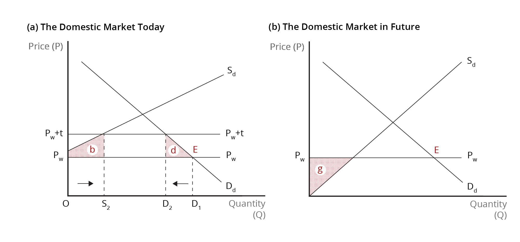
In Figure 7.3, we analyze the economic effects of an export subsidy in the case of a small exporting country. Recall that a small country has no influence over the world price of the product. Prior to any engagement in international trade, the product price in the domestic market is given by the intersection of the supply and demand curves. The small country can export any quantity of the product at the higher world price. Before the government grants the export subsidy, consumers purchase  and domestic producers supply
  at the world price. The difference between the quantity supplied and the quantity demanded, i.e.,
  , represents the initial level of exports,
  .
.
Once the export subsidy is granted, the price domestic producers receive on export sales rises and is equal to the world price plus the subsidy. While the payment of the subsidy applies only to exports, the price on domestic sales of the product also rises to the world price plus the export subsidy. There is no reason the producers will accept a lower price on domestic sales since they can sell as much of the product as they want at the higher world price. With the domestic price now higher, consumers reduce the quantity they purchase to  while producers expand their output to
  . Therefore, the level of exports rise to
  or
or  .
.
The export subsidy, therefore, increases output and exports as producers respond to the higher price. Producer surplus increases by the sum of areas  ,
,  , and
, and  , as they sell a larger quantity and the receive a higher price. On the other hand, consumers lose surplus equal to area
  , since they pay a higher price and buy a smaller quantity. The cost of the export subsidy is the subsidy
 ") times the quantity of exports, and is equal to area
times the quantity of exports, and is equal to area  .
.
We can combine all of these effects – on producers, consumers, and the government budget – to evaluate the economic effects for the country as a whole. This is done in Table 7.1.
Table 7.1 Summary of the Economic Effects of an Export Subsidy in a Small Country | Item | Gain/Loss |
| Producer surplus gain or loss |  |
| Consumer surplus gain or loss |  |
| Export subsidy |  |
| National economic well-being |  |
Combining these effects, we see that national economic well-being is reduced as a result of the subsidy, with the net national loss being equal to the sum of areas and . Area is the consumption effect of the export subsidy as consumers are squeezed out of the market by the increase in the domestic price. Area  is the production effect of the export subsidy which arises because the government has chosen to encourage domestic production that has a resource cost that is higher than the world price. The loss of national economic well-being for our small exporting country is also a loss to the world.
What about the impact of the export subsidy in importing countries?
The Effects of an Export Subsidy for a Large Country
We analyze the economic effects of an export subsidy for a large exporting country in Figure 7.4. A large country can influence the world price of the product given its large share of the global market. Prior to any engagement in international trade, the price of the product in the domestic market is given by the intersection of the supply and demand curves. Before the government grants the export subsidy, consumers purchased and domestic producers supplied at the world price. The difference between the quantity supplied and the quantity demanded, i.e., , represents the initial level of exports, .
After the export subsidy is granted, the price that foreign consumers pay for the product falls below the world price. This is because exporters in the large country are wanting to increase exports to get bigger subsidy payments. To entice foreign consumers to buy more of the product, exporters must lower the export price. With the export price falling below the world price, exporters effectively share the subsidy with foreign buyers. The price that domestic consumers pay is equal to the price that foreign buyers pay – the export price – plus the export subsidy.
Given the increase in the domestic price, consumers in the exporting country reduce the quantity they purchase from to . Meanwhile, domestic producers increase their output from to . Thus, the level of exports increases to , the difference between and . Domestic consumers are worse off due to the export subsidy since they lose surplus equal to the sum of areas and . Producers, in contrast, experience a gain in their surplus equal to the sum of areas , and . The surplus that consumers lose is transferred to producers as a gain. The cost of the export subsidy is given by the quantity of exports times the subsidy and is given by the combined area  .
.
We can add up the changes in consumer surplus, producer surplus, and the government budget to evaluate the impact of the export subsidy on the economic well-being of the nation. This is done in Table 7.2. We see that national economic well-being is reduced as a result of the export subsidy. Part of the cost of the export subsidy represents a transfer to the producers of the export good and remains within the country. The remainder of the subsidy payment is a benefit to foreign consumers as they pay a lower price and buy a larger quantity.
We can divide the net national loss to the exporting country into three parts – the consumption effect (area ), the production effect (area ), and the loss due to the decline in the country’s terms of trade (the combined area  ). In addition, the export subsidy has a negative impact on world well-being. This results from the deadweight losses of the production effect and the consumption effect in the exporting country and the fact that the resource cost of the additional imports was higher that the value that foreign consumers put on them.
Table 7.2 Summary of the Economic Effects of an Export Subsidy in a Large Country | Item | Gain/Loss |
| Producer surplus gain or loss | |
| Consumer surplus gain or loss | |
| Export subsidy |  |
| National economic well-being |  |
References
Carbaugh, R.J. (2015). International economics, (15th ed.). Cengage Learning.
Pugel, T. A. (2020). International economics, (17th ed.). McGraw-Hill.
Image Descriptions
Figure 7.1: An Illustration of International Price Discrimination
The image shows two side-by-side graphs with ‘Price’ on the vertical axis and ‘Quantity’ on the horizontal axis.
On the left, the graph labelled ‘Domestic Market’ includes a downward-sloping demand curve labelled ‘D’; from the same origin at the top of the y-axis, the Marginal Revenue curve labelled ‘MR’ slopes downward to the left of D. A horizontal line one-third up the y-axis is labelled ‘MC = AC’. The equilibrium price, P*, and quantity, Q*, on the axes are connected by a dotted horizontal and vertical line that both pass through the MR line to meet the demand curve. A tall, red-shaded rectangle is formed by the y-axis, MC=AC, Q* and P*; the triangle formed to the right of MR passing through the rectangle is labelled Profit.
On the right, the graph labelled ‘Foreign Market’ includes a downward-sloping demand curve labelled ‘D’; from the same origin in the middle of the y-axis, the Marginal Revenue curve labelled ‘MR’ slopes downward to the left of D. A horizontal line one-third up the y-axis is labelled ‘MC = AC’. The equilibrium price, P*, and quantity, Q*, on the axes are connected by a dotted horizontal and vertical line that both pass through the MR line to meet the demand curve. A short, red-shaded rectangle is formed by the y-axis, MC=AC, Q* and P*; the triangle formed to the right of MR passing through the rectangle is labelled Profit.
Rectangle and subsequent Profit triangle in the Foreign Market graph is less than one third the size as in the Domestic Market graph.
[back]
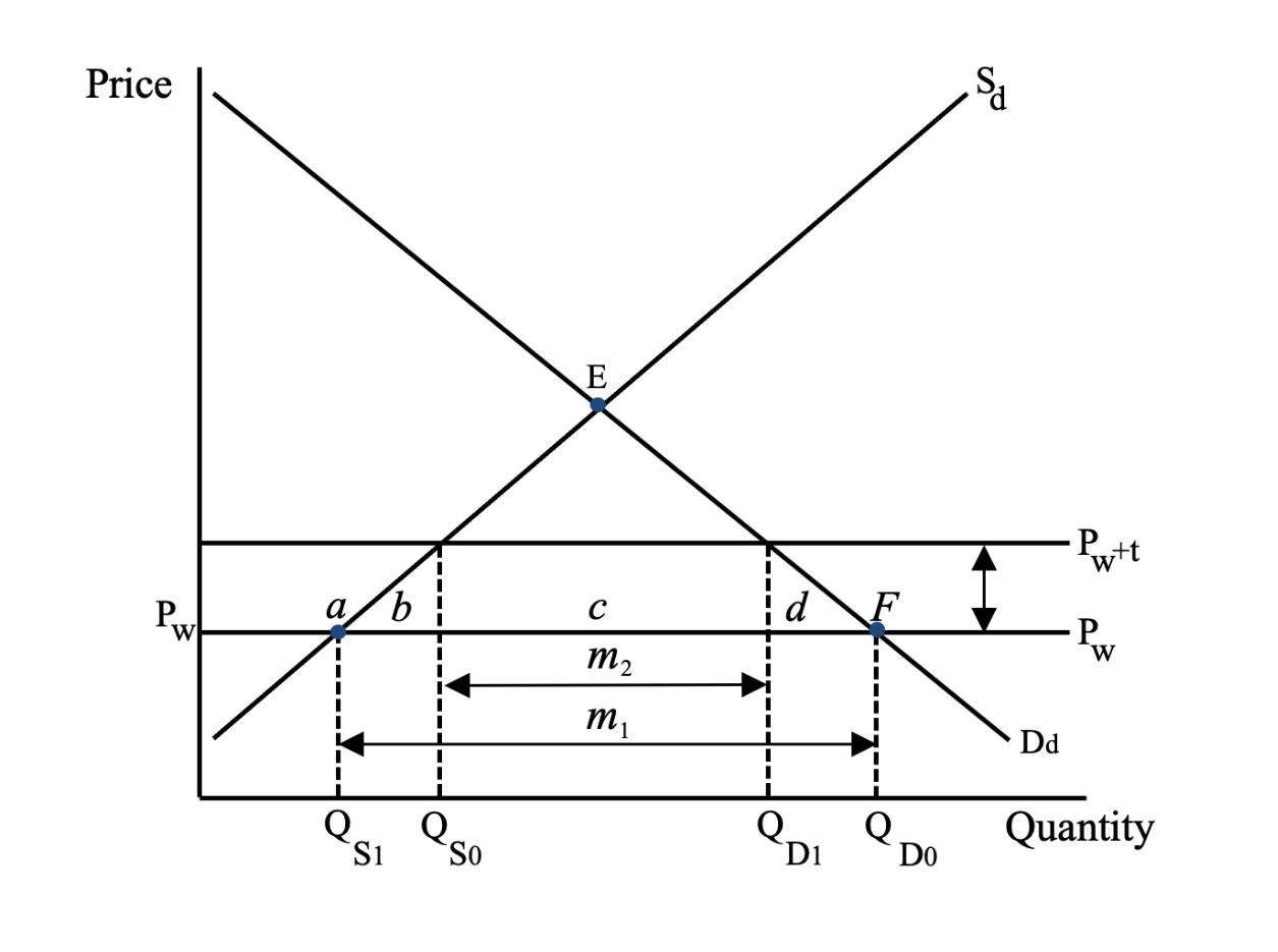
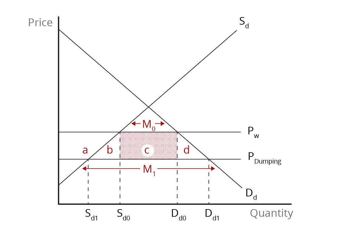
Figure 7.2: The Economic Effects of Dumping in Small Importing Country
The image is a graph with the x-axis labelled “Quantity,” and the y-axis labelled “Price.” Two intersecting lines form an X in the graph: the downward-sloping line is labelled “D,” and the upward-sloping line is labelled “S.” A horizontal line below the intersection of supply and demand point is labelled “PW.” Below it, another horizontal line is labelled “Pd” Four points on the quantity axis are labelled from left to right as “Qs1,” “Qs0,” “Qd0,” and “Qd1.” At each intersection of supply, demand, and the price lines are dotted vertical lines down to the points on the quantity axis.
Area a is above the intersection of S and Pd and below PW. Area b is the triangle formed by S, Pd and Qs0. Area c is the rectangle in the middle formed by QS0, PW, Qd0 and Pd. Area d mirrors b, formed by Qd0, Pd, and D.
[back]
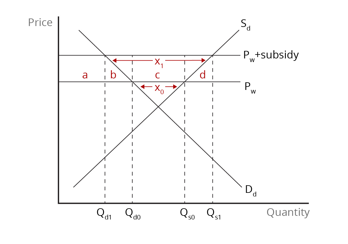
Figure 7.3: The Effects of an Export Subsidy for a Small Exporting Country
The image is a graph with the x-axis labelled “Quantity” and the y-axis labelled “Price.” Two intersecting lines form an X in the graph: the downward-sloping line is labelled “Dd,” and the upward-sloping line is labelled “Sd.” A horizontal line above the intersection of supply and demand point is labelled “PW.” Above it, another horizontal line is labelled “Pw + subsidy.” Four points on the quantity axis are labelled from left to right as “Qd1,” “Qd0,” “Qs0,” and “Qs1.” At each intersection of supply, demand, and the price lines are dotted vertical lines down to the points on the quantity axis.
Area a is the rectangle formed by the y-axis, Pw, Qd1, and Pw + subsidy. Area b is the triangle formed by Qd1, Pw, and Dd. Area c is the rectangle in the middle formed by Qd0, PW, Qs0 and Pw + subsidy. Area d mirrors b, formed by Sd, Pw, and Qs1.
The triangle formed above the intersection of Sd and Dd and below Pw is marked with a double-sided arrow between Sd and Dd and labelled X0. Above Pw, a double-sided arrow between Sd and Dd is labelled X1.
[back]
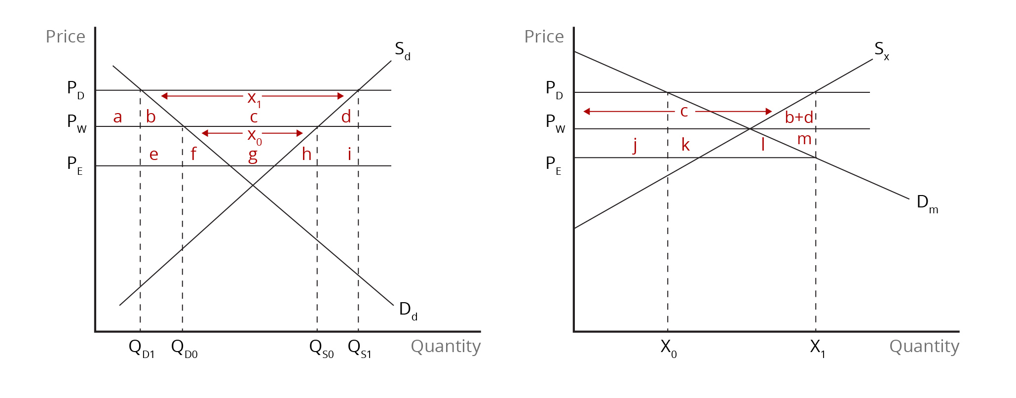
Figure 7.4: The Effect of an Export Subsidy for a Large Exporting Country
The image shows two side-by-side graphs with ‘Price’ on the vertical axis and ‘Quantity’ on the horizontal axis.
On the left graph, two intersecting lines form an X in the graph: the downward-sloping line is labelled “Dd,” and the upward-sloping line is labelled “Sd.” A horizontal line above the intersection of supply and demand point is labelled “PE.” Above it is another horizontal line is labelled “PW.” Above that is a third horizontal line labelled “PD”
Four points on the quantity axis are labelled from left to right as “QD1,” “QD0,” “QS0,” and “QS1.” At each intersection of supply, demand, and the price lines are dotted vertical lines down to the points on the quantity axis.
Areas a through d are contained between PD and PW. Area a is the square formed by the y-axis, PD, QD1, and Pw. Area b is the triangle formed by QD1, PW, and Dd. Area c is the trapezoid in the middle formed by Dd, PW, Sd, and PD. Area d mirrors b, formed by Sd, PW, and Qs1.
Areas e through i are contained between PW and PE. Area e is the square formed by the QD1, PE, QD0, and PW. Area f is the triangle formed by QD0, PE, and Dd. Area g is the trapezoid formed in the middle by Dd, PE, Sd, and PW. Area h mirrors e, formed by Sd, PE, and Qs0. Area i mirrors area e and is a square formed by the QS0, PE, QS1, and PW.
Between Sd and Dd and below PD is a horizontal double-sided arrow labelled X1. Between Sd and Dd and below PW is a horizontal double-sided arrow labelled X0.
On the right graph, two intersecting lines form an X in the upper half of the graph: the downward-sloping line is labelled “Dm,” and the upward-sloping line is labelled “SX.” A horizontal line above the intersection of supply and demand point is labelled “PD.” A horizontal line through the intersection of the supply and demand curves is labelled “PW.” Below is a third horizontal line labelled “PE” which does not extend past its intersection with the demand curve.
Two points on the quantity axis are labelled from left to right as “X0” and “X1.” A horizontal dotted line extends up from X0 to the intersection of PD and DM. A horizontal dotted line extends up from X1 through the intersection of PE and DM, ending at the intersection of PD and SX.
Area c is formed by the y-axis, PW, SX, and PD and is marked with a double-sided arrow to show its span across the demand curve. Area b+d is the triangle formed right of SX by PW and X1. Area j is the rectangle formed by the y-axis and X0, between PE and PW. Area K is to the right of X0, in the space between PE, SX and PW. Area i is the triangle below the intersection of SX and DM formed by PE. Area m is the triangle formed right of DM by PW and X1.
[back]


 Consumption

 is the change,
  is quantity, and
  is price.


 is quantity, and


 ), then Canada is capital-abundant, and the other country is capital-scarce. A product is resource-intensive if the resource cost represents a greater share of its value than it does for other products (Pugel, 2020). If
 m} >\text{(K/L)a}") , where
, where  and
and  denote manufacturing and agriculture, respectively, then the manufacturing industry is capital-intensive, and agriculture is labour-intensive. When a resource is abundant, its relative cost is low, and the prices of the products that intensively use that resource will also be low. This, of course, makes sense intuitively: If a country has a lot of a resource, then that resource will be relatively cheap, and if a significant amount of that resource is used in production, then the resulting products will also be cheap.
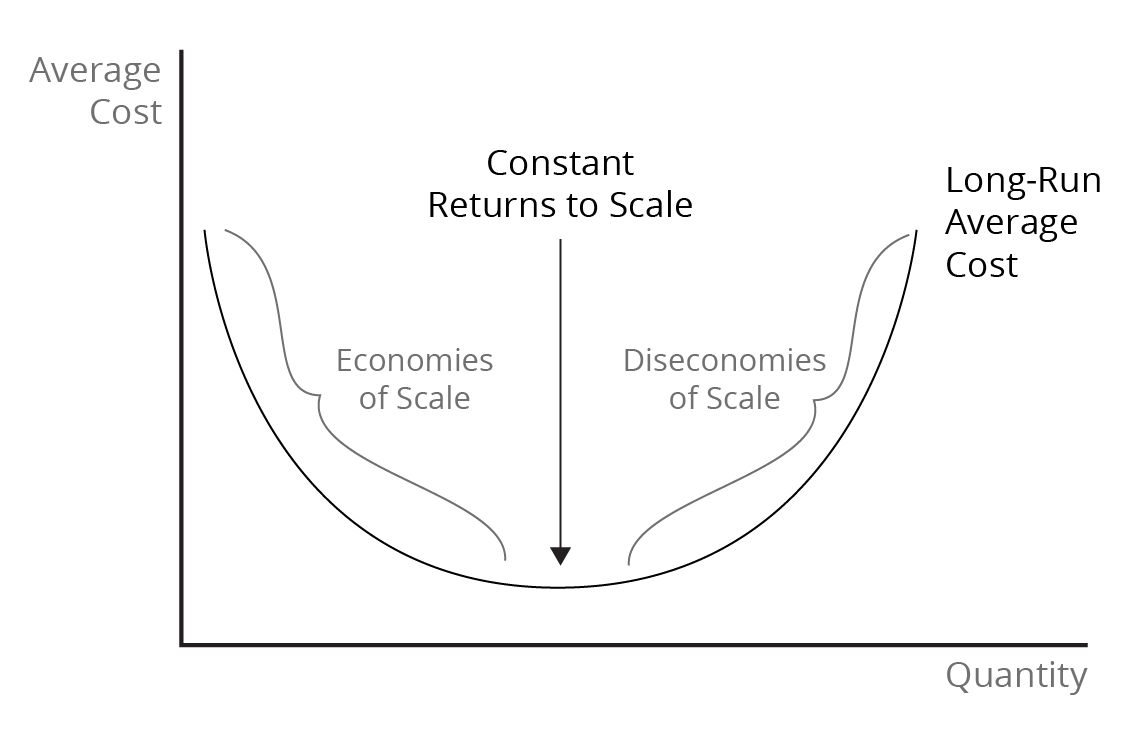
 (see Figure 3.2). The former represents the demand side of the market, and the average cost curve represents its supply side. The price curve relates the number of product varieties on the horizontal axis to the price of the broad product. With only a very limited number of varieties available, the product price is relatively high. However, as more and more product varieties become available on the market, the typical firm loses pricing power, as each new variety represents a substitute and, therefore, an increase in competition. Price, therefore, falls with the introduction of more and more product varieties. The price curve, therefore, is downward sloping. It is also relatively flat, indicating a considerable degree of competition in the market.
 and
and  , are given by the intersection of the price and unit cost curves. At the point of intersection, price is equal to average total cost, and firms in the industry are earning zero economic profit in long-run equilibrium. This represents the situation prior to trade, as depicted in Figure 3.2.
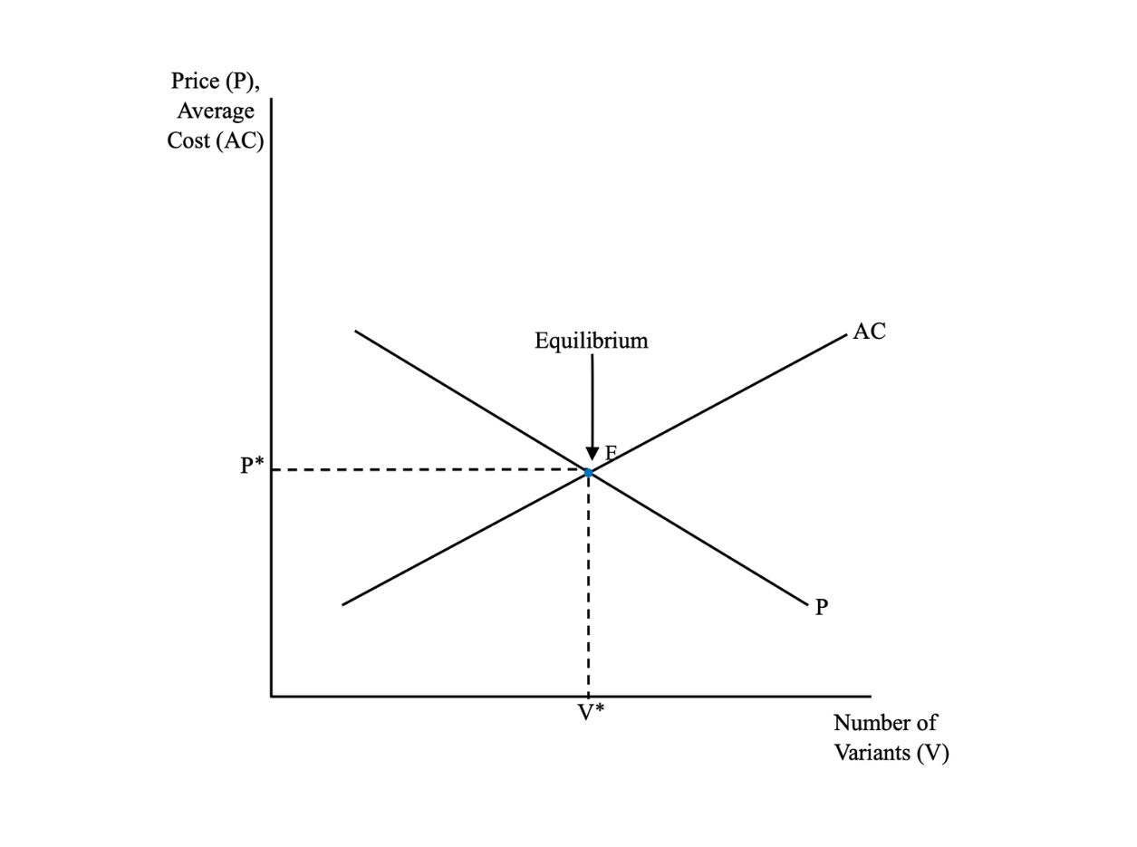
}") lies further to the right than the
lies further to the right than the 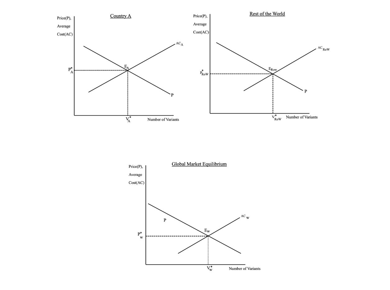
![[(v' - v)/v]*\text{100}](https://atu0g9ctah.execute-api.ca-central-1.amazonaws.com/latest/latex?latex=%5B%28v%27%20-%20v%29%2Fv%5D%2A%5Ctext%7B100%7D&fg=000000&font=TeX&svg=1 "[(v' - v)/v]*\text{100}")
 is a unit value added before the tariff on imported inputs is applied, and
  is a unit value added after the tariff on imported inputs is applied (Pugel, 2020).
")
![[(v' - v)/v]*\text{100}]](https://atu0g9ctah.execute-api.ca-central-1.amazonaws.com/latest/latex?latex=%5B%28v%27%20-%20v%29%2Fv%5D%2A%5Ctext%7B100%7D%5D&fg=000000&font=TeX&svg=1 "[(v' - v)/v]*\text{100}]")
 ) and demand (
 ) curves. We determine equilibrium in the domestic market by the intersection of the demand and supply curves at point
  . If the economy is opened to international trade, it can import an unlimited amount of the product at the going world price. That is, the supply of imports is constant at the world price, shown as a horizontal line lying below the domestic equilibrium market price before trade. At the world price, the domestic market equilibrium shifts from Point E to Point F, where the demand curve intersects the world price line,
  . At this point, the total quantity of the product that is purchased is
  , and the quantity supplied by domestic producers is
  .
. , where
  is the import tariff. As a result, consumers cut back on purchases of the product to
  , as they bear the full burden of the tariff; producers expand their production to
  due to the protective effect of the tariff; and the quantity of imports fall from their pre-tariff levels to the difference between
  . Producer surplus rises by area
 ![[(\text{Q}_{S1}-\text{Q}_{D1})*\text{t}]](https://atu0g9ctah.execute-api.ca-central-1.amazonaws.com/latest/latex?latex=%5B%28%5Ctext%7BQ%7D_%7BS1%7D-%5Ctext%7BQ%7D_%7BD1%7D%29%2A%5Ctext%7Bt%7D%5D&fg=000000&font=TeX&svg=1 "[(\text{Q}_{S1}-\text{Q}_{D1})*\text{t}]") . While tariff revenue represents a loss to consumers, it is not a loss to the nation as there is a transfer of surplus from consumers to the national government. The tariff revenue is captured by area
. While tariff revenue represents a loss to consumers, it is not a loss to the nation as there is a transfer of surplus from consumers to the national government. The tariff revenue is captured by area 


 and the domestic supply is given by
  . The intersection of supply and demand in the importing country before trade determines the equilibrium price and quantity. When the domestic market opens up to international trade, the importing country faces an international price of
  . With free trade, equilibrium in the domestic markets shifts. Domestic consumers now purchase
  and domestic producers supply
  . The difference between the quantity purchased and the quantity supplied domestically represents the initial quantity of imports.
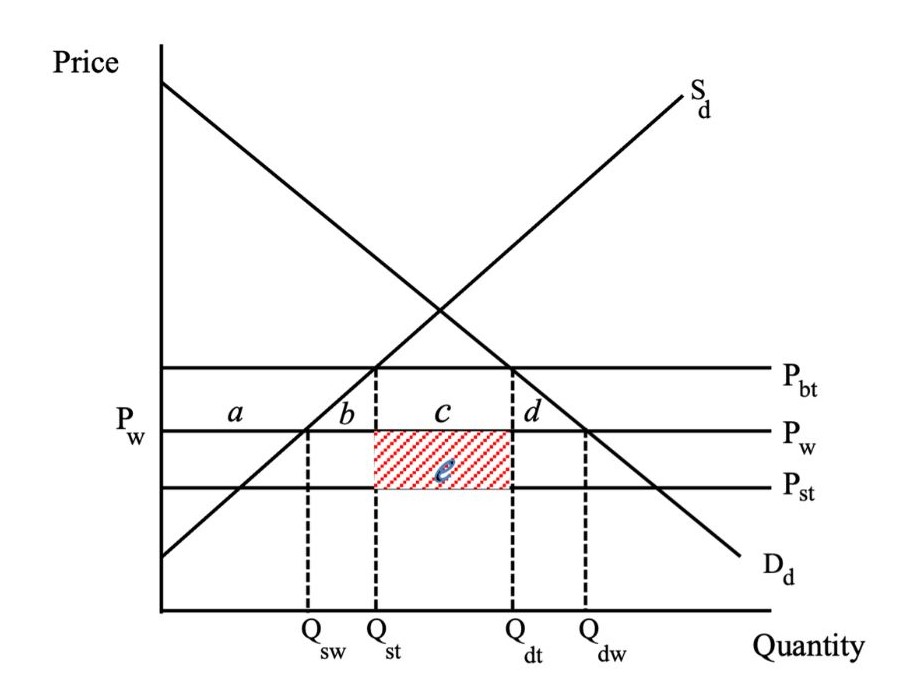
 . The increase in the domestic price leads to an increase in domestic production from
  to
to  and a reduction in domestic consumption from
  to
to  . As a result, the quantity of imports falls to the difference between
  , lies below the world price,
  . With the tariff is equal to the vertical difference between the price line
  . Here, we can see that a portion of the tariff revenue is collected from domestic consumers, equal to area
  , the importing country is better off as a result of the tariff. If
")
 , where the demand curve intersects the world price line,
  , where
  represents the quota quantity. For the quota to be effective, the level of imports must be set lower than that which would have occurred in the absence of free trade. Since supply is now reduced below the free-trade level, the domestic price rises above the world price and is given by the intersection of the “new” supply curve,
  (parallel to the world price,
  . Consumers are worse off compared with the free-trade situation as they must pay a higher price and get a smaller quantity. Graphically, consumer surplus falls by areas
  and they receive a higher price. As a result, producer surplus increases by area
  ) represents the initial quantity of imports prior to the imposition of the quota.
") , supply comes only from domestic producers; above the world price line, the domestic supply
, supply comes only from domestic producers; above the world price line, the domestic supply ") increases by the extent of the quota (i.e., the quota quantity). The pertinent domestic supply curve with international trade now becomes
increases by the extent of the quota (i.e., the quota quantity). The pertinent domestic supply curve with international trade now becomes  ).
).") is indicated by the horizontal line – parallel to and above the world price,
is indicated by the horizontal line – parallel to and above the world price,  . With the large importing country able to exercise buying power, the price received by foreign suppliers in the import market
 ") lies parallel to and below the world price.
lies parallel to and below the world price. to
to  and a reduction in domestic consumption from
  to
to  . As a result, the quantity of imports falls to the difference between
  , lies below the world price,
  and
and ") multiplied by the quota mark-up or the sum of area
multiplied by the quota mark-up or the sum of area 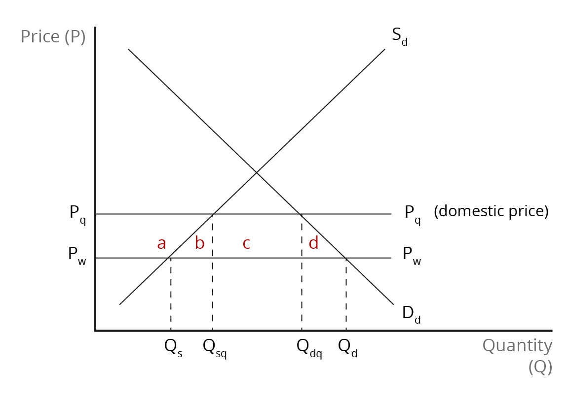
") increases by the extent of the quantity allowed under the VER. The pertinent domestic supply curve with international trade now becomes
increases by the extent of the quantity allowed under the VER. The pertinent domestic supply curve with international trade now becomes  , where
 ") represents the quantity under the VER. For this quantity restriction to be effective, the level of imports must be set lower than that which would have occurred in the absence of free trade. Since supply is now reduced below the free-trade level, the domestic price rises above the world price and is given by the intersection of the “new” supply curve,
represents the quantity under the VER. For this quantity restriction to be effective, the level of imports must be set lower than that which would have occurred in the absence of free trade. Since supply is now reduced below the free-trade level, the domestic price rises above the world price and is given by the intersection of the “new” supply curve,  . The domestic price is indicated by the horizontal line,
 ") , parallel to and above the world price,
, parallel to and above the world price,  and they receive a higher price. As a result, producer surplus increases by area
  area
area 
") in Panel (a) of Figure 6.2. In light of its inability to influence the world price, the small country can purchase any amount of the product at the prevailing world price
in Panel (a) of Figure 6.2. In light of its inability to influence the world price, the small country can purchase any amount of the product at the prevailing world price  and the quantity supplied is
  . The difference between
  , where
  is the tariff. The higher domestic price causes domestic consumers to buy a smaller quantity,
  and domestic producers to boost their level of production to
  . As a result, the level of imports falls from
  to
to  . The small country suffers the usual deadweight losses of the production effect (area
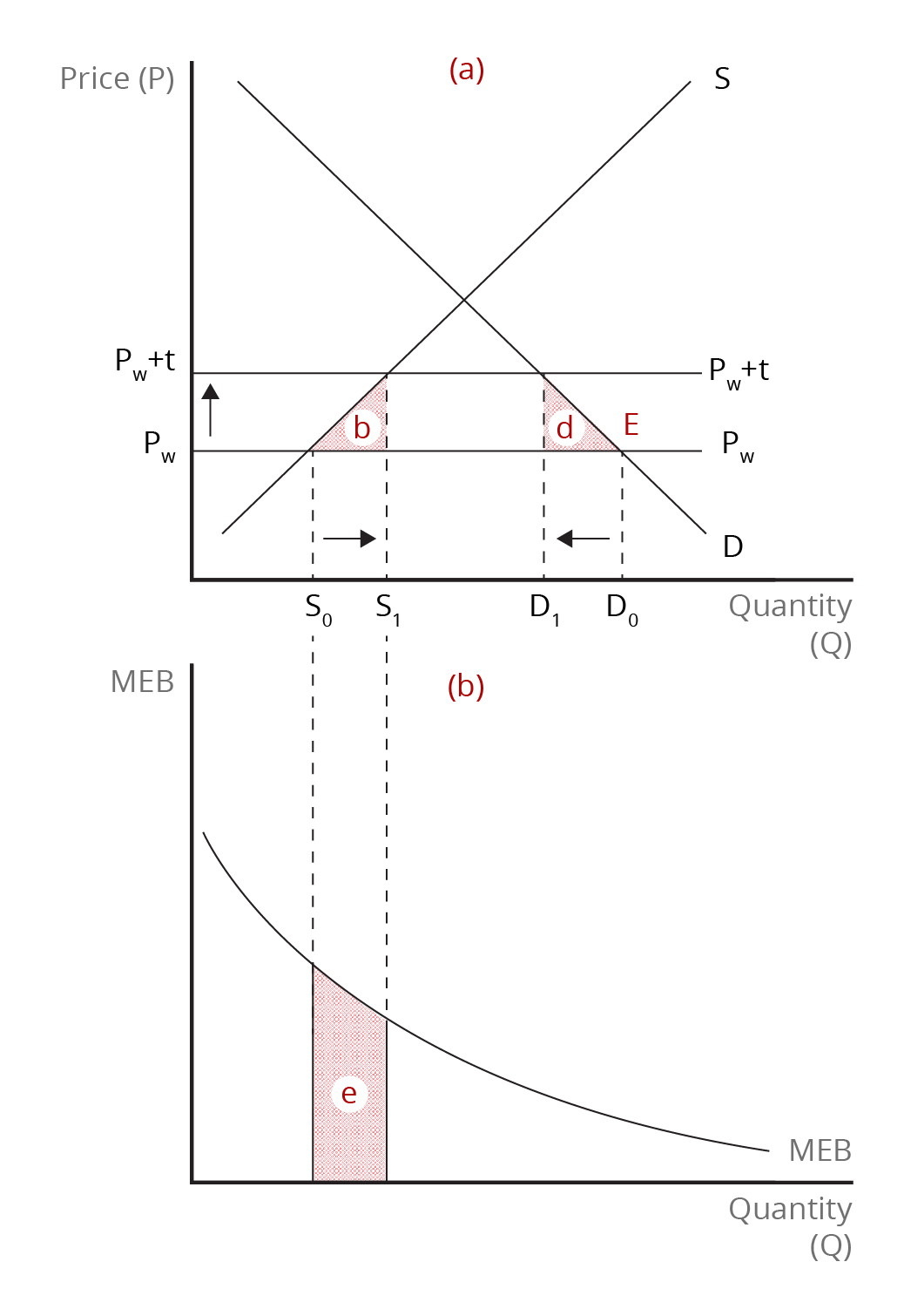
 , where
  represents the subsidy. On the assumption that the subsidy is equivalent to the import tariff, producers respond by boosting production to the same extent. As in the case of the tariff, higher-cost domestic production is substituted in consumption for lower-cost imports. With domestic production increasing from
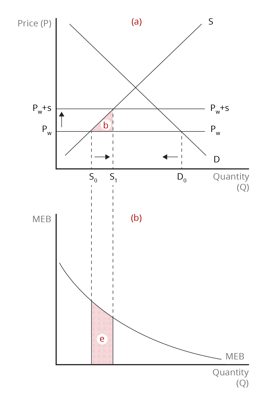
 , where
  and consumers reduce the quantity they purchase from
  . Thus, the quantity of imports falls from
  to
to  . With the import tariff allowing domestic production to begin, the usual deadweight losses due to the production effect and the consumption effect are incurred. Initially, therefore, the small country would experience the usual net national loss in economic well-being from tariff protection. This situation is depicted in Figure 6.4 (a).
 has been created.
 area
area ") . Even so, import protection may not be the most appropriate policy. A policy that gets to the root of the problem may be superior because it reduces economic loss. Since there is no reason to make imports more costly for consumers, thereby reducing consumption, a production subsidy which avoids the consumption effect will be better.
. Even so, import protection may not be the most appropriate policy. A policy that gets to the root of the problem may be superior because it reduces economic loss. Since there is no reason to make imports more costly for consumers, thereby reducing consumption, a production subsidy which avoids the consumption effect will be better.") and the reduction in imports after the imposition of the tariff. If another policy was used to grant import protection to domestic producers, such as a quota, the tariff-equivalent can be approximated by the difference between the domestic price and the world price. For a small country, the net national loss from tariff protection is given by the following expression:
and the reduction in imports after the imposition of the tariff. If another policy was used to grant import protection to domestic producers, such as a quota, the tariff-equivalent can be approximated by the difference between the domestic price and the world price. For a small country, the net national loss from tariff protection is given by the following expression:
 and the reduction in imports is
  , where
  is the free-trade quantity of imports and
  is the quantity of imports after the imposition of the tariff.
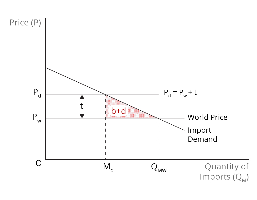

![\frac{1}{2}\times\textit{[Reduction in Import Quantity]}\times\textit{[Tariff Rate (%)}\times\textit{Import Price}]](https://atu0g9ctah.execute-api.ca-central-1.amazonaws.com/latest/latex?latex=%5Cfrac%7B1%7D%7B2%7D%5Ctimes%5Ctextit%7B%5BReduction%20in%20Import%20Quantity%5D%7D%5Ctimes%5Ctextit%7B%5BTariff%20Rate%20%28%25%29%7D%5Ctimes%5Ctextit%7BImport%20Price%7D%5D&fg=000000&font=TeX&svg=1 "\frac{1}{2}\times\textit{[Reduction in Import Quantity]}\times\textit{[Tariff Rate (%)}\times\textit{Import Price}]")
![\frac{1}{2}\times\frac{\textit{[Reduction in Import Quantity]}}{\textit{[Import Quantity]}}\times\textit{[Tariff Rate}\times\textit{Import Price]}\times\textit{[Import Quantity]}](https://atu0g9ctah.execute-api.ca-central-1.amazonaws.com/latest/latex?latex=%5Cfrac%7B1%7D%7B2%7D%5Ctimes%5Cfrac%7B%5Ctextit%7B%5BReduction%20in%20Import%20Quantity%5D%7D%7D%7B%5Ctextit%7B%5BImport%20Quantity%5D%7D%7D%5Ctimes%5Ctextit%7B%5BTariff%20Rate%7D%5Ctimes%5Ctextit%7BImport%20Price%5D%7D%5Ctimes%5Ctextit%7B%5BImport%20Quantity%5D%7D&fg=000000&font=TeX&svg=1 "\frac{1}{2}\times\frac{\textit{[Reduction in Import Quantity]}}{\textit{[Import Quantity]}}\times\textit{[Tariff Rate}\times\textit{Import Price]}\times\textit{[Import Quantity]}")
![\frac{1}{2}\times\textit{[Percent Reduction in Import Quantity]}\times\textit{[Tariff Rate (%)}\times\frac{[\textit{Import Value}]}{\textit{GDP}}](https://atu0g9ctah.execute-api.ca-central-1.amazonaws.com/latest/latex?latex=%5Cfrac%7B1%7D%7B2%7D%5Ctimes%5Ctextit%7B%5BPercent%20Reduction%20in%20Import%20Quantity%5D%7D%5Ctimes%5Ctextit%7B%5BTariff%20Rate%20%28%25%29%7D%5Ctimes%5Cfrac%7B%5B%5Ctextit%7BImport%20Value%7D%5D%7D%7B%5Ctextit%7BGDP%7D%7D&fg=000000&font=TeX&svg=1 "\frac{1}{2}\times\textit{[Percent Reduction in Import Quantity]}\times\textit{[Tariff Rate (%)}\times\frac{[\textit{Import Value}]}{\textit{GDP}}")
") . Note that this estimate is based on a significant reduction in imports and a comparatively high share of the imported product in GDP. As this example shows, the net national loss from import protection is unlikely to be large for countries that have low tariffs and are not particularly dependent on imports.
. Note that this estimate is based on a significant reduction in imports and a comparatively high share of the imported product in GDP. As this example shows, the net national loss from import protection is unlikely to be large for countries that have low tariffs and are not particularly dependent on imports.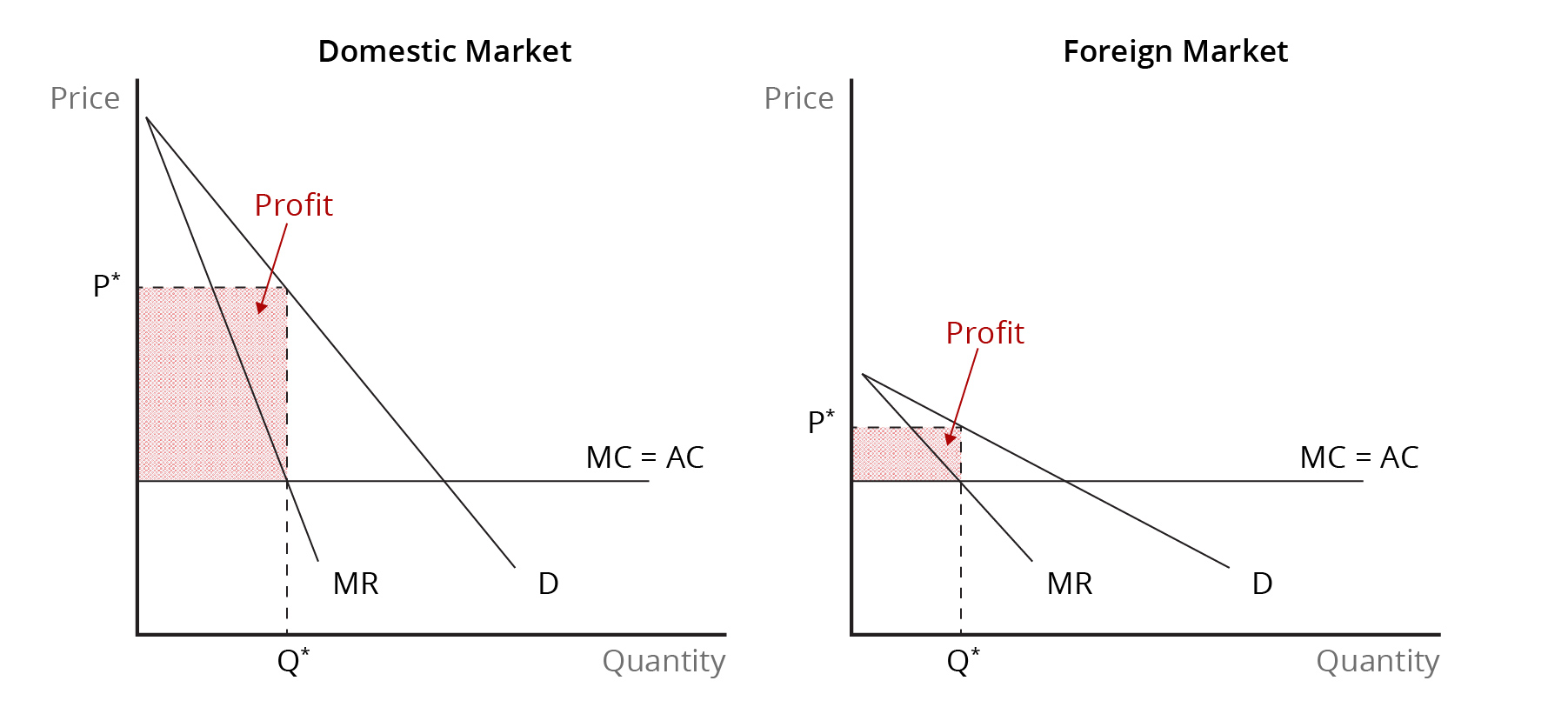
 at the world price,
  . Since the quantity demanded is greater that the quantity supplied domestically, the difference,
  , represents the quantity of imports,
  . With dumping taking place in the domestic market, the price of the imported product falls below the world price. This price is represented by the price line
  . As a result of the lower price, domestic consumers buy a larger quantity while domestic producers scale back their production. Imports, therefore, increase to
  .
.
") , producers
, producers ") , and the government
, and the government ") , we see that the net national loss is the sum of area b and d, the production and consumption effects. The countervailing duty is good for the world as it eliminates inefficient overproduction but bad for the importing country. If we compare the situation of the export subsidy and the countervailing duty with free trade (i.e., the situation before the export subsidy is given), the difference is that the importing country’s government now receives revenue from the duty. The exporting country is, in effect, transferring subsidy payments into the coffers of the importing-country government. The well-being of the importing country with the countervailing duty is higher than under free trade.
, we see that the net national loss is the sum of area b and d, the production and consumption effects. The countervailing duty is good for the world as it eliminates inefficient overproduction but bad for the importing country. If we compare the situation of the export subsidy and the countervailing duty with free trade (i.e., the situation before the export subsidy is given), the difference is that the importing country’s government now receives revenue from the duty. The exporting country is, in effect, transferring subsidy payments into the coffers of the importing-country government. The well-being of the importing country with the countervailing duty is higher than under free trade.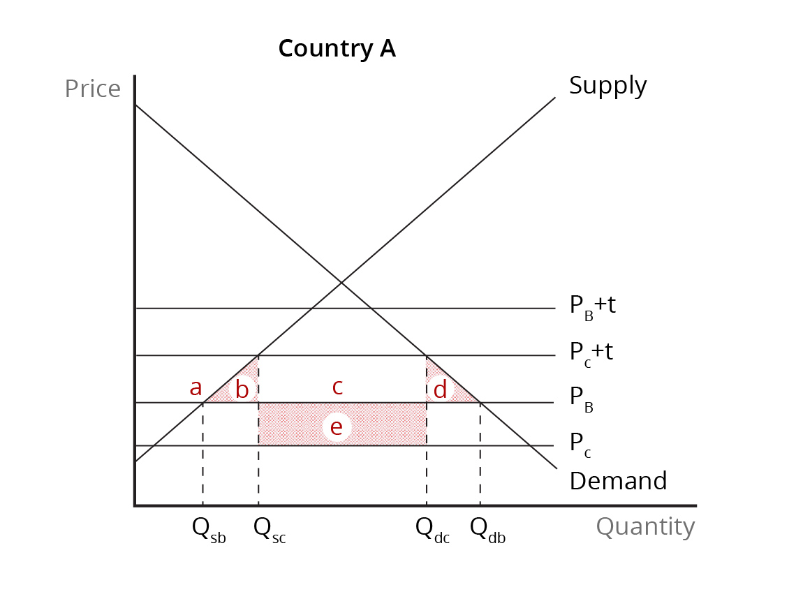
 , where
  . At the lower price of
  while consumers purchase
  , with the difference between these two quantities being imports.
 , as only the more efficient domestic producers can supply the product. Meanwhile, the quantity purchased rises to
  . The quantity of imports, therefore, increases. There is clearly an increase in trade as a result of the customs union. This trade creation results because higher-cost production of a member of the customs union (Country A) is replaced by lower cost imports from another member (Country B). This represents an increase in well-being for Country A because consumer surplus rises and there has been an efficiency gain in production. Trade creation is the sum of the production effect (area
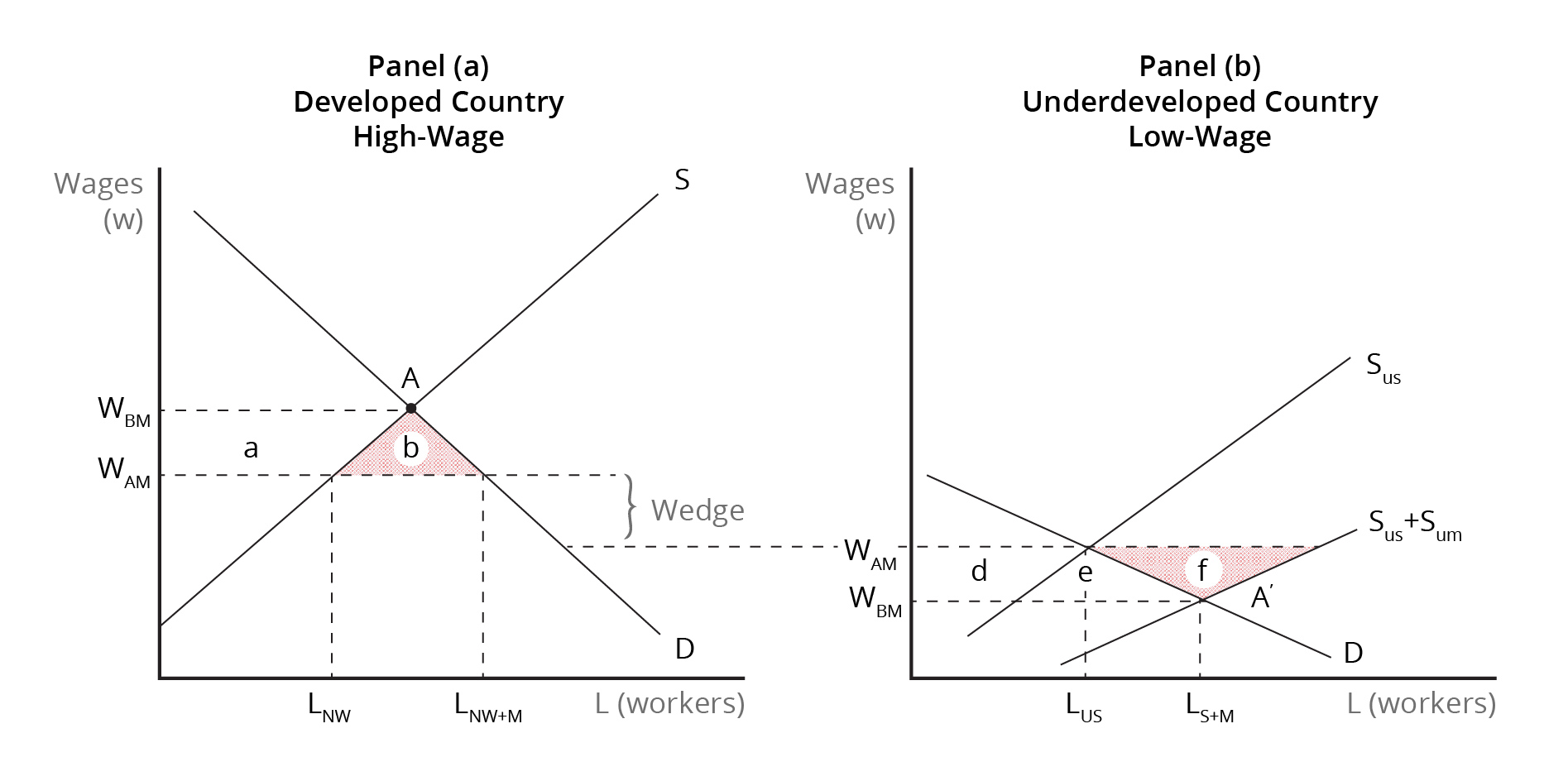
 , and the demand for labour is given by
  . The intersection of the supply and demand curves gives a high wage rate in equilibrium (
 ) at point
  . The labour market in the underdeveloped country is shown in Panel (b) in Figure 8.2 using a similar supply and demand diagram. However, in the case of an underdeveloped country, the supply of labour is segmented to distinguish the workers who are left after migration has taken place. The workers who stay
 ") plus the workers who migrate
plus the workers who migrate ") make up the total supply of labour
make up the total supply of labour ") . The intersection of the total labour supply and the demand curve in the underdeveloped country gives a low wage rate in equilibrium
. The intersection of the total labour supply and the demand curve in the underdeveloped country gives a low wage rate in equilibrium ") at point
at point  .
. . As a result, there is a fall in the quantity of labour employed from
  to
to  . These workers, therefore, gain economic surplus equal to area
  . As a result, they lose economic surplus equal to area a. What workers in this country lose, area
  in Panel (b) of Figure 8.2. Part of what the migrant workers gain, area
  .
.