Learning Objectives
Operate the Plant at 80% capacity burning coal to
- Perform combustion analyses for two types of coal,
- Compare results.
Theory
In the Boiler Efficiency lab, we stated that Combustion Efficiency is defined as the ratio of the burner’s capability to burn fuel completely to the unburned fuel and excess air in the exhaust. In this lab, we will perform a combustion analysis.
Fossil fuels may be classified into solid, liquid and gaseous fuels. The vast majority of fuels are based on carbon (C), hydrogen (H2) or some combination of carbon and hydrogen called hydrocarbons.
During combustion, oxygen (O2) combines rapidly with C, H2, sulphur (S2) and their compounds in solid, liquid and gaseous fuels and results in the liberation of energy. Except for special applications such as oxyacetylene welding, in which a high-temperature flame is required, the O2 necessary for combustion is obtained from air. Air contains O2 and nitrogen (N2), plus negligible amounts of other gasses and for engineering purposes, may be considered to have the following percentage composition by mass:
O2: 23%
N2: 77%
The proportions in which the elements enter into the combustion reaction by mass are dependent upon the relative molecular weights as shown below:
| Element | Symbol | Molecular Weight |
| Carbon | C | 12 |
| Sulphur | S2 | 32 |
| Hydrogen | H2 | 2 |
| Oxygen | O2 | 32 |
| Nitrogen | N2 | 28 |
Stoichiometric Combustion Theory
Complete combustion of simple hydrocarbon fuels forms carbon dioxide (C02) from the carbon and water (H20) from the hydrogen, so for a hydrocarbon fuel with the general composition CnHm, the combustion equation on a molar basis is as flows:

Where the balance should be satisfied following the moles for any mathematcial equation:
Carbon balance:
 kmol CO2/ kmol fuel
Hydrogen balance:

 kmol H2O/ kmol fuel
Oxygen balance:

 kmol O2/ kmol fuel
Considering that combustion occurs in air rather than in pure oxygen, the nitrogen in the air may react in the combustion process to produce nitrogen oxides. Beside, some fuels contain elements other than carbon, and these elements may react with oxygen during combustion. Also, combustion is not always complete, and the exhaust gases contain unburned and partially burned products in addition to C02 and H2O.
Air is composed of oxygen, nitrogen, and small amounts of carbon dioxide, argon, and other trace components. For the purposes of the further calculation it is perfectly reasonable to consider air as a mixture of 21% (mole basis) 02 and 79 % (mole basis) N2. Nitrogen will be considered as an “inert” gas in the combustion calculations. The stoichiometric relation for complete combustion of a hydrocarbon fuel, CnHm, becomes

The balance equations are:
Carbon balance:
kmol CO2/ kmol fuel
Hydrogen balance:
kmol H2O/ kmol fuel
Oxygen balance:
kmol O2/ kmol fuel
Nitrogen balance:
 kmol N2/kmol fuel
Flue gas compositions are presented in terms of mole fractions as kmol of product per kmol of fuel.
Example 1. Combustion of Octane in Air
Determine the stoichiometric air/ fuel mass ratio and product gas composition for combustion of octane ( C8H18) in air.

Carbon balance:
 kmol CO2/ kmol fuel
Hydrogen balance:

 kmol H2O/ kmol fuel
Oxygen balance:
+b")
 kmol O2/ kmol fuel
Nitrogen balance:
 kmol N2/kmol fuel
The combustion equation becomes:

Air/ fuel mass based ratio considering that 1 kmol fuel is 114 kg of fuel ( 8*12 + 18 *(1) = 114):

Flue gas composition on molar basis is:
Total number of kmol of flue gasses = kmol CO2 + kmol H2O + kmol N2 = 8 +9+ 47 = 64 kmol flue gasses/ kmol fuel
CO2 = 8/64 = 12.5 %
H2O = 9/64 = 14 %
N2 = 47/64 = 73.5%
Other components and impurities in the fuel make the calculation process more complicated. For example if sulfur exists in fuel it is usually combust into sulfur dioxide (SO2). Ash, the noncombustible inorganic (mineral) impurities in the fuel, undergoes a number of transformations at combustion temperatures, will be neglected in the further calculation (ash will be assumed to be inert).
For most solid and liquid fuels, the chemical composition is on a mass basis, as determined in the ultimate analysis.
Mass Based Chemistry of Combustion
The combustion reactions are written following the stoichiometric rules as defined above. The quantity of matter entering into a reaction is equal to the quantity of matter in the products of the reaction.
The reaction for the complete combustion of C may be written as follows:
C+O2=CO2
or, if molecular weights are used,
12+32=44
1 kg C + 2⅔ kg O2 = 3⅔ kg CO2
The complete combustion of H2 occurs as follows:
2H2 +O2 =2H2O
4+32=36
1 kg H2 + 8 kg O2 = 9 kg H2O
Sulphur burns as follows:
S +O2 =SO2
32+32=64
1 kg S + 1 kg O2 = 2 kg SO2
In addition, 1 kg of O2 (stoichiometric mass of O2) is contained in 1/0.232=4.3 kg air which is the stoichiometric mass of air. This air will contain 4.3-1=3.3 kg N2. Therefore we can write:
1 kg S + 4.3 kg air = 2 kg SO2+3.3 kg N2
Procedure
If the analysis of fuel is given by mass, follow the steps below:
- Total O2 required: Determine the mass of O2 required for each constituent and find the total mass of O2 (Subtract any O2 which may be in the fuel)
- Stoichiometric air: Stoichiometric mass of air = O2 required/0.232
- Total mass of combustion products: Determine the % mass of each combustion product. For example, given C content of 84.9%, CO2=84.9/100*2⅔=3.11% and find the total mass of combustion products.
- Analysis of combustion products by mass: Suppose the total mass of combustion products in step 3 has been found as 12.09 kg/kg fuel, then CO2=3.11/12.09*100=25.74. This means that 25.74% of the flue gas is CO2. Repeat this calculation for each constituent.
Lab Instructions
Run the initial condition I14 80% Coal and setup trends for the following variables:
X00820 X00821 X00822 X00823 X00824 E23356
G02196 G02197 X32419 X02419 G00831 H00830
- Burning default coal: After 10 minutes of running the simulator, freeze simulator and print the two trends. This is the reference point for the next step.
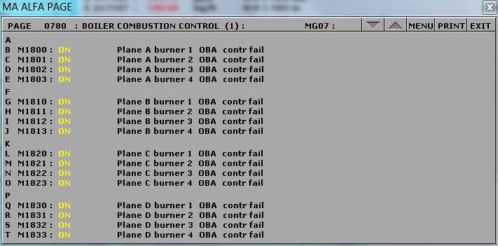
- Burning poor quality coal: Switch to run mode and access Variable List page 0111 on MD180. Set the new values as shown below. After 10 minutes, freeze simulator and print the two trends.
- X00820: 70.40
- X00821: 5.10
- X00822: 1.10
- X00823: 12.50
- X00824: 1.60
- X00825: 9.30
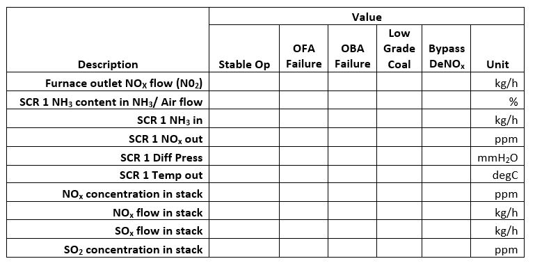
- Computation: Compute the following values for both types of fuels:
- Total O2 required
- Stoichiometric air
- Total mass of combustion products
- Analysis of combustion products by mass [%]: CO2, H2O, SO2, N2
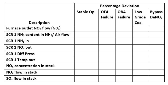
- Comparison: Compare your findings based on the following data:
- Furnace outlet SOx flow
- Furnace outlet NOx flow
- CO content in flue gas
- Oxygen content in flue gas
- Theoretical combustion air
- Coal Heat Value
Hints & Tips
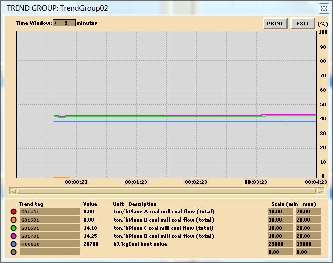
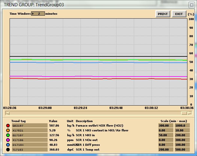
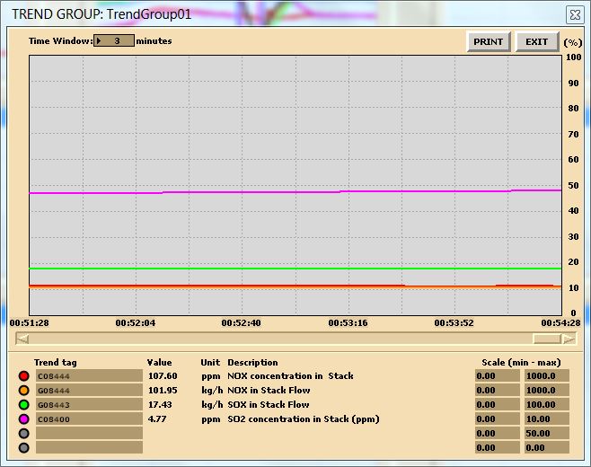
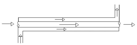
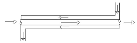
In this lab, you are carrying out two combustion analyses. For data collection, set up your trends, a sample trend plot is shown below (Make sure your trend printouts are labeled properly otherwise, data analysis will be very confusing):
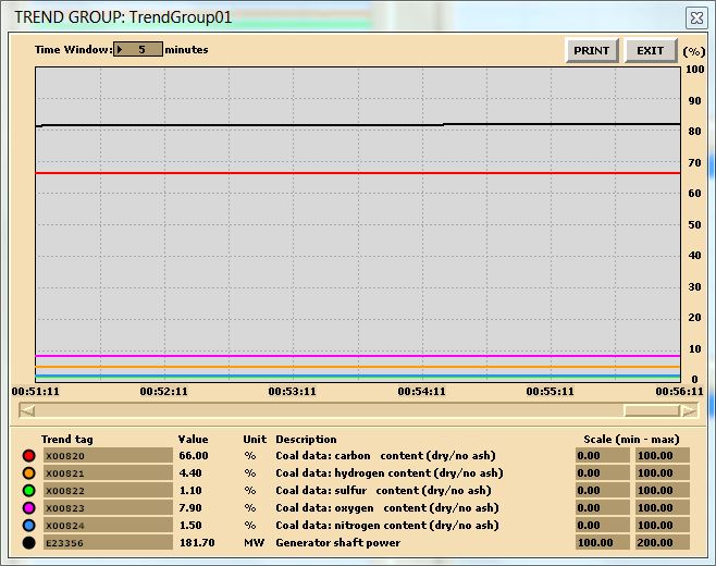
Sample data for coal
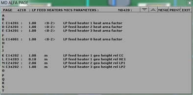
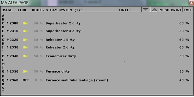
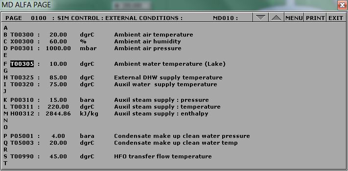
To change the fuel composition use the Variable List Page#: 0111 on MD180:
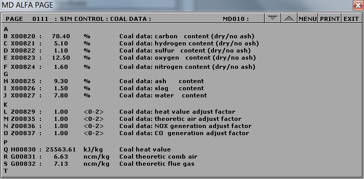
Chemical composition of coal
Deliverables
Your lab report is to include the following:
- Trend plots: Supply all plots taken for each of the 2 fuels,
- Computation: As per lab instructions above, perform combustion analyses using MATLAB or MS Excel.
- Conclusion: Write a summary (max. 500 words, in a text box if using Excel) comparing your results and suggestions for further study.
Further Reading:
- Basic Engineering Thermodynamics in SI Units by R. Joel: Combustion.
- Thermal Engineering by H.L. Solberg, O.C. Cromer and A.R. Spalding: Fossil fuels and their combustion.
Stoichiometry.


}{m_{f}HV}100\%")

}{(H_{1}-H_{2})}")


-(h_{4}-h_{3})}{(h_{1}-h_{4})}")


}{R_{T}}")
(LMTD)")


")