For each entry the chapter in which the word first appears is shown in parentheses.
A
aa (4) a lava flow that solidifies with a blocky high-relief surface
ablation (16) melting of ice in the context of glaciation
ablation till (16) till that is formed when englacial and supraglacial sediments are deposited because the ice that was supporting them melts
abyssal plain (18) the flat surface of the deep ocean, typically beyond the limits of the continental slopes
abyssalpelagic zone (18) the deeper parts of the ocean, between 4000 and 6000 m.
accretion (plate tectonics) (21) the process by which continental blocks (terranes) are added to existing continental areas
accretion (planetary) (22) the process by which solid celestial bodies are added to existing bodies during collisions
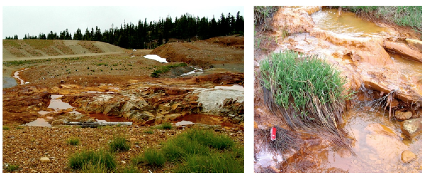
acid rock drainage (5) the production of acid from oxidation of sulphide minerals (especially pyrite) in either naturally or anthropogenically exposed rock
aeolian (6) processes related to transportation and deposition of sediments by wind
aerobic (18) processes that take place in the presence of abundant oxygen
aerosol (4) an aggregate of fine solid particles or a small droplet of liquid suspended in the air
aftershock (11) an earthquake that can be shown to have been caused by another earthquake
aggregate (20) unconsolidated materials (typically sediments) that are used in the construction industry
albedo (19) the reflectivity of a surface of a planet (expressed as the percentage of light that reflects)
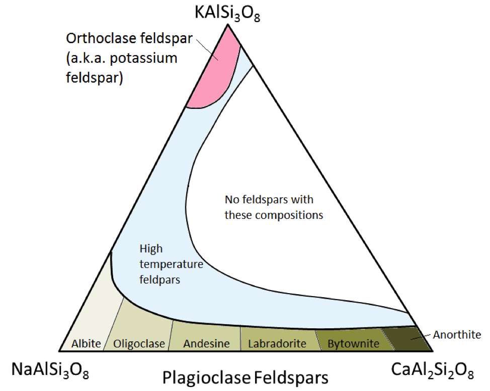
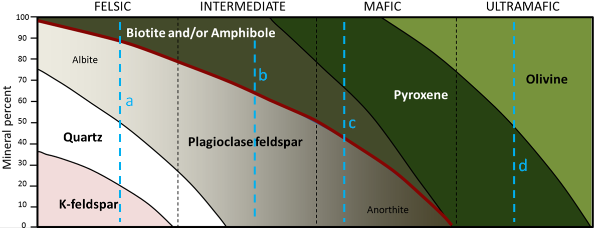
albite (2) sodium-rich plagioclase feldspar
alpine glacier (16) a glacier formed in a mountainous region and confined to a valley (same as valley glacier)
amphibole (2) a double-chain ferromagnesian silicate mineral (e.g., hornblende)
amphibolite (7) a foliated metamorphic rock in which the mineral amphibole is an important component
amplification (11) in the context of seismic shaking the process by which the amplitude of the seismic waves are enhanced, especially because the
amplitude (17) for any type of wave, the difference in height between a crest and the adjacent trough
anaerobic (18) processes that take place without oxygen
andesite (3) a volcanic rock of intermediate composition
anion (2) a negatively charged ion
angular unconformity (8) a geological boundary at the base of a sedimentary layer where the sedimentary rock beneath has been tilted or folded and then eroded
anorthite (2) calcium-rich plagioclase feldspar
Antarctic Bottom Water (18) water at abyssal depths in the ocean that forms from the sinking of dense cold water adjacent to Antarctica
anticline (12) an upward fold where the beds are known not to be overturned
anthracite (20) a high grade of coal (92 to 98% carbon) that is formed from deep burial and weak metamorphism
anthropogenic (19) resulting from the influence of humans
antiform (12) an upward fold where it is not known if the beds have been overturned
aphanitic (3) an igneous texture characterized by crystals that are too small to see with the naked eye
aquifer (14) a body of rock or sediment that has sufficient permeability to allow it to be used as a source of groundwater
aquitard (14) a body of rock or sediment that has insufficient permeability to allow it to be used as a source of groundwater
arch (17) a rock weathering remnant in the form of an arch (typically along a coast and resulting from wave erosion)
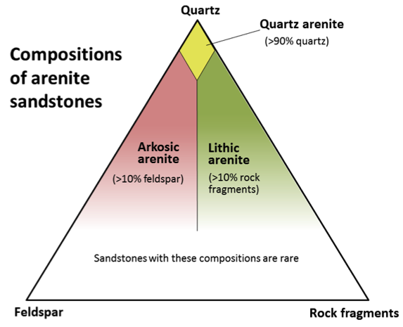
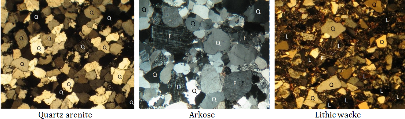
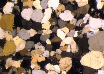
arenite (6) a sandstone with less than 15% silt and clay
arete (16) a sharp ridge that separates adjacent glacially carved valleys
arkose (6) a sandstone with more than 10% feldspar and more feldspar than lithic fragments
arkosic arenite (6) an arkose with less than 15% clay/silt matrix
artesian well (14) a well that is completed in a confined aquifer and in which the water level in the well rises above the top of the aquifer
asteroid (22) a rocky body orbiting the Sun
asteroid belt (22) the region between the orbits of Mars and Jupiter that is populated with many asteroids
asthenosphere (1) the part of the mantle, from about 100 to 200 km below surface, within which the mantle material is close to its melting point, and therefore relatively weak
asymmetrical (12) in the context of folds, where the two sides of the fold make significantly different angles with respect to the axial plane
atoll (18) a ring-shaped carbonate (or coral) reef or series of islands
atomic mass (2) the total number of neutrons plus protons in an atom
atomic number (2) the total number of protons in an atom
attitude (12) the orientation of a sloping geological feature, such as a bedding plane or fracture
auerole (7) a zone of metamorphism around a source of heat such as a magma body
axial plane (12) a plane that can be traced through all of the hinge lines of a fold
B
back reef (6) the zone of shallow water on the shore-side of a reef
background (geochemistry) (20) the typical level of an element in average rocks or sediments
backwash (17) the wash of wave water down the slope of a beach
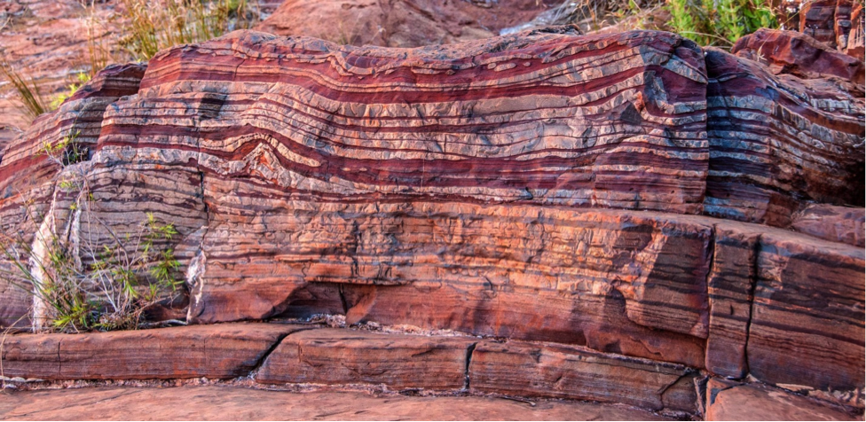
banded iron formation (6) an iron-bearing sedimentary rock that is rich in minerals such as hematite and magnetite, which may be interbedded with chert
bank-full stage (13) the water level of stream when it is in flood and just about to flow over its banks
barrier reef (18) a carbonate (or coral) reef that forms a barrier to waves along a coast
basal sliding (16) the motion of glacial ice along the base of a glacier that is warm enough to have liquid water
basalt (1) a volcanic rock of mafic composition
base level (13) in the context of a stream the base level is the lowest level that it can erode down to, as defined by the ocean, a lake or another stream that it flows into
batholith (3) an irregular body of intrusive igneous rock that has an exposed surface of at least 100 km2
bathypelagic zone (18) the moderately deep parts of the ocean, between 1000 and 4000 m.
baymouth bar (17) a spit that extends across the mouth of a bay
beach face (17) the part of the beach that is relatively steep and lies between the high and low tide levels
bed (6) a sedimentary layer
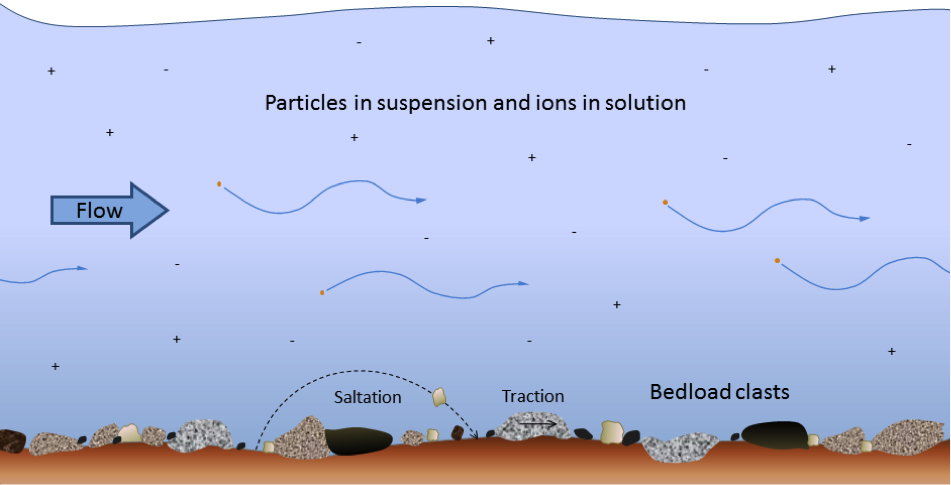
bed load (6) the fraction of a stream’s sediment load that typically rests on the bottom and is moved by saltation and traction
bedding (6) repeated layering in a sedimentary rock
bentonite (15) a type of smectite clay that has strong swelling properties and is effective at absorbing dissolved ions
berm (17) a flat area of a beach in the backshore area (above the high tide level)
big-bang theory (22) the theory that the universe started with a giant explosion approximately 13.77 billion years ago
biotite (2) a sheet silicate mineral (mica) that includes iron and or magnesium, and is therefore a ferromagnesian silicate
biozone (8) a stratigraphic interval that can be defined on the basis of a specific fossil
bituminous (20) a medium-grade type of coal with 70 to 92% carbon
blueschist (7) a metamorphic facies characterized by relatively low temperatures and high pressures, such as can exist within a subduction zone
body wave (9) a seismic wave that travels through rock (e.g., a P-wave or an S-wave)
boulder (6) a sediment clast with a diameter of at least 256 mm
Bowen reaction series (3) the scheme that defines the typical order of crystallization of minerals from magma
braided (13) a stream pattern which is characterized by abundant sediment and numerous intertwining channels around bars
breakwater (17) a structure built offshore in order to deflect the energy of waves
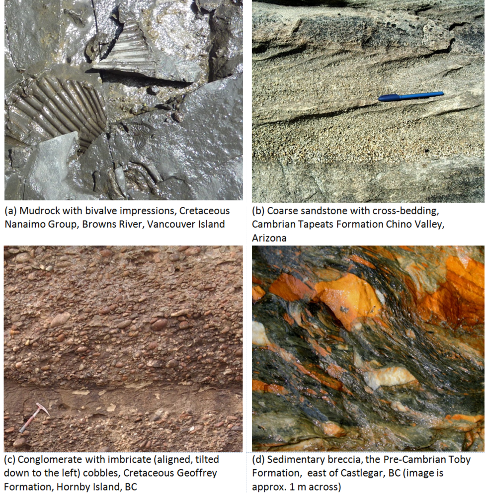
breccia (6) a sedimentary- or volcanic-rock texture characterized by angular clasts
brunisol (5) a relatively immature forest soil, lacking in well-defined horizons
C
caldera (4) a volcanic depression that is many times larger than the volcanic vents within it
caliche (5) a white calcium-carbonate rich layer within soils in arid regions
calving (16) the loss of ice from the front of a glacier by collapse into water
Canadian Shield (21) the exposed part of the continent Laurentia
carbonate (2) a mineral in which the anion is CO3-2
carbonate compensation depth (18) the depth in the ocean (typically around 4000 m) below which carbonate minerals are soluble
cation (2) a positively charged ion
cementation (6) the process by which minerals are precipitated between grains in sediments
Cenozoic (1) the most recent of the eras, representing the past 65.5 Ma of geological time
chemical sedimentary rock (6) a sedimentary rock comprised of material that was transported as ions in solution
chernozem (5) a black soil typical of grasslands in cold climates such as the Canadian Prairies
chert (6) a very fine grained sedimentary rock formed almost entirely of silica
chlorite (2) a ferromagnesian sheet silicate mineral, typically present as fine crystals and forming from the low-temperature metamorphism of mafic rock
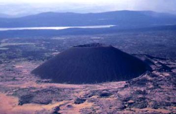
cinder cone (4) a steep-sided volcano comprised almost entirely of loose rock fragments and typically formed during a single eruptive event
cirque (16) a steep-sided semi-circular basin eroded by a glacier at the head of its valley
clast (6) a sedimentary fragment of mineral or rock
clastic sedimentary rock (6) a sedimentary rock comprised of material that was transported as clasts or fragments
clay (6) sediment particle that is less than 1/256 mm in diameter
clay mineral (6) a hydrous sheet silicate mineral that typically exists as clay-sized grains
claystone (6) a sedimentary rock comprised mostly of clay-sized grains
cleavage (2) the tendency for a mineral to break along smooth planes that are predetermined by its lattice structure
climate feedback (19) a process by which the physical effects of a climate forcing can have other effects (either negative or positive) on the climate
climate forcing (19) a mechanism, such as a change in greenhouse gas levels, that forces the climate to change
coal-bed methane (20) methane that is trapped within the porosity of coal
coastal straightening (17) the tendency for an irregular coast to be straightened over time by coastal erosion processes
cobble (6) sediment particle that is between 64 and 256 mm in diameter
col (16) the low point or pass along a ridge between two glacial valleys
columnar jointing (4) the fracturing of rock or sediment (but typically volcanic rock) into columns that are typically 6-sided
composite volcano (or stratovolcano) (4) a volcano that is constructed of alternating layers of pyroclastic debris and lava flows
concentrate (mining) (20) a product of ore processing that includes a specific ore mineral, separated from the rest of the rock
concordant (3) parallel to pre-existing layering or foliation within a rock
cone of depression (14) the depression of the water table around a well that is heavily pumped
confined aquifer (14) an aquifer that lies below a confining layer
confining layer (14) an aquitard that overlies an aquifer and restricts the flow of water down from the surface
conglomerate (6) a sedimentary rock that is comprised predominantly of rounded grains that are larger than 2 mm
contact metamorphism (7) metamorphism that takes place adjacent to a source of heat, such as a body of magma
continental drift (10) the concept that tectonic plates can move across the surface of the Earth
continental glacier (16) a glacier that covers a significant part of a continent and has an area of at least 50,000 km2
continental shelf (18) the shallow (typically less than 200 m) and flat sub-marine extension of a continent
continental slope (18) the steeper part of a continental margin, that slopes down from a continental shelf towards the abyssal plain
contractionism (10) the now discredited theory that mountain ranges formed as a result of the contraction of the Earth
convergent boundary (10) a plate boundary at which the two plates are moving towards each other
Cordilleran Ice Sheet (16) the continental glacier that covered part of western North America, including almost all of British Columbia, part of the Yukon, and part of northern Washington, during the Pleistocene glaciations
core (1) the metallic interior part of the Earth, extending from a depth of 2900 km to the centre
core-mantle boundary (9) the boundary, at 2900 km depth, between the mantle and the core
Coriolis effect (18) the tendency for moving bodies (e.g., ocean currents) to rotate on the surface of the Earth, clockwise in the northern hemisphere and counter-clockwise in the southern hemisphere
cosmic microwave background (22) radiation left over from the an early stage in the development of the universe at the time when protons and neutrons were recombining to form atoms
country rock (3) the original rock of a region, into which younger rock (typically igneous) rock has been intruded
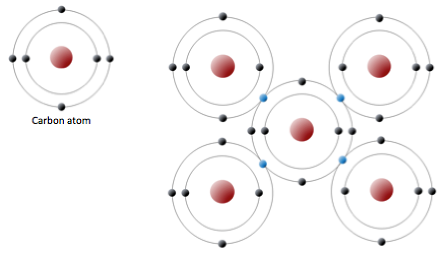
covalent bond (2) a bond between two atoms in which electrons are shared
crater (4) a volcanic depression that is related to a specific volcanic vent
craton (21) a region of ancient (typically Precambrian) crystalline rock (equivalent to a shield)
creep (15) the very slow (mm to cm per year) flow of unconsolidated material on a gentle slope
crest (17) the highest point on a wave
crevasse (16) an open fissure on the surface of a glacier
cross bedding (6) small-scale inclined bedding within larger horizontal beds
crust (4) the uppermost layer of the Earth, ranging in thickness from about 5 km (in the oceans) to over 50 km (on the continents)
cyanobacteria (6) photosynthetic bacteria that evolved in the early Archean
D
D” layer (9) (d-double-prime layer) a low seismic velocity zone within the basal 200 km of the mantle
debris flow (15) a gravity-driven flow of water and sediment that includes a significant proportion of coarse (cobble to boulder) material
decline (20) in mining a decline is a sloped tunnel used to access lower parts of a mine with wheeled equipment
decompression melting (3) melting (or partial melting) of rock resulting from a reduction in pressure without a significant reduction in temperature
dendritic (13) a pattern of drainage channels that resembles the branches in a tree
density (2) weight per volume of a substance (e.g., g/cm3) used widely in the context of minerals or rocks
deranged (13) a pattern of drainage channels that is chaotic
detrital (6) referring to fragments of rocks or minerals
diatom (18) photosynthetic algae that make their tests (shells) from silica
differentiation (22) the un-mixing of a magma, typically by the physical separation of minerals that crystallize early and settle towards the bottom
diorite (3) an intermediate intrusive igneous rock
dip (12) the angle below horizontal at which a sedimentary bed or other feature slopes
discharge (6) the volume of water flow in a stream expressed in terms of volume per unit time (e.g., m3/s)
discharge area (14) the part of an aquifer where groundwater discharge takes place
disconformity (8) a boundary between parallel sedimentary layers where some erosion of the lower layer has taken place
discordant (3) a geological feature that is not parallel to any existing layering in the country rock
divalent (2) an ion with a charge or +2 or -2
divergent (10) a plate boundary at which the two plates are moving towards away from each other
dodecahedron (2) an object with twelve surfaces, such as a garnet crystal
dolomite (6) a calcium-magnesium carbonate mineral (Ca,Mg)CO3
dolomitization (6) the addition of magnesium to limestone during which some or all of the calcium carbonate is converted to dolomite
dolostone (6) a carbonate rock made up primarily of the mineral dolomite
drainage basin (13) the catchment area of a stream, including the area where all surface water drains into the stream
drop stone (16) a fragment of rock within otherwise fine-grained sediment that has been dropped from floating ice on a body of water
drumlin (16) a streamlined glacial erosional feature comprised of sediments and/or bedrock
dyke (3) a tabular intrusive igneous body that is discordant to any existing layering in the country rock
E
eccentricity (19) in the context of Milankovitch Cycles, the degree to which the Sun is offset from the geometric centre of the Earth’s orbit
eclogite (7) a garnet-pyroxene-glaucophane bearing rock that is the product of high-pressure metamorphism of oceanic crustal rock, typically within a subduction zone
effusive (4) a volcanic eruption dominated by the relatively gentle flow of lava
El Niño (19) a periodic climatic situation in which warm water extends all or most of the way to the eastern edge of the equatorial Pacific
elastic deformation (11) the deformation of material (including rock) from which it can fully recover if the stress is removed
electron (2) a sub-atomic particle of essentially no mass and a single negative charge
end moraine (16) a deposit of sediment that accumulates at the front of a glacier
englacial (16) within a glacier, referring especially to sediment carried within the glacial ice
epicentre (11) the location on the surface vertically above the location (i.e., “hypocentre” or “focus”) where an earthquake takes place
epipelagic zone (18) the upper layer of water (0 to 200 m) in areas of the open ocean
epithermal deposit (20) a mineral deposit formed near to surface in an area of hydrothermal activity, typically associated with a body of magma
equilibrium line (16) on a glacier, the line between the zone of accumulation and the zone of ablation (in late summer the equilibrium line is the boundary between snow-covered ice and bare ice)
equipotential lines (14) in the context of groundwater an equipotential line connects locations with equal hydraulic head or water pressure
esker (16) a ridge of sediment deposited by a sub-glacial stream
eustatic sea level change (17) sea level change related to a change in the volume of the oceans, typically because of an increase or decrease in the amount of glacial ice on land
exfoliation (5) the fracturing of rock that results from a reduction in the pressure when overlying rock is eroded away
exoplanet (22) a planet that orbits a star other than the Sun
extrusive (3) igneous rock that cooled at surface
F
fall (15) in mass wasting, the vertical or near-vertical fall of rock
fault (12) a boundary in rock or sediment along which displacement has taken place
feedback (19) a process by which the physical effects of a climate forcing can have other effects (either negative or positive) on the climate
feldspar (2) a very common framework silicate mineral
felsic (3) silica rich (>65% SiO2) in the context of magma or igneous rock
ferric (2) the oxidized form of an ion of iron (Fe3+)
ferromagnesian (2) referring to a silicate mineral that contains iron and or magnesium
ferrous (2) the reduced (non-oxidized) form of an ion of iron (Fe2+)
fetch (17) the distance over which wind blows to form waves
finger lake (16) a lake that occupies a glacial valley
firn (16) the granular transitional state between snow and ice within a glacier
flood plain (13) the area that is occupied by water when a stream floods and overtops its banks
flow (15) the fluid-like motion of material during mass-wasting
flow path (14) the path that groundwater flows along between a recharge area and a discharge area
flowing artesian well (14) an artesian well in which the water level naturally rises above the surface of the ground
flux melting (3) melting of rock that is facilitated by the addition of a flux (typically water) which lowers the rocks melting point
focus (earthquake) (11) the actual point below surface at which an earthquake takes place (equivalent to hypocentre)
foliated (7) the existence of foliation in a metamorphic rock
foliation (7) the alignment of mineralogical or structural features of a rock – especially a metamorphic rock
footwall (12) the lower surface of a non-vertical fault
foraminifera (18) a single-celled protist with a shell that is typically made of CaCO3
fore-reef (6) the zone on the ocean side of a reef
formation (6) a unit of sedimentary rock that is lithologically consistent and sufficiently thick and extensive to be shown on a geological map at the scale that is typically used in the area in question
fracking (20) fracturing rock by injecting water and chemicals down a well at very high pressure (equivalent to hydraulic fracturing)
fractional crystallization (3) the sequential crystallization of minerals from magma, and the physical separation of early-forming crystals from the magma in the area where they crystallized
fracture (2) a break within a body of rock in which the rock on either side is not displaced
fringing reef (18) a reef adjacent to a shoreline where there is either a very narrow back reef area or none at all (in which case the reef is effectively attached to the shore)
frost line (22) in the context of planetary systems the boundary beyond which volatile components (e.g., water, carbon dioxide, methane, ammonia etc.) are frozen
frost wedging (5) the situation where the expansion of freezing water pries rock apart
G
Ga (1) (gigaannus) billions of years before the present
gabbro (3) a mafic intrusive igneous rock
Gaia hypothesis (19) the hypothesis advanced by James Lovelock that the organisms have affected the atmosphere and oceans such that conditions on Earth have been kept habitable, in spite of significantly changing energy received from the Sun
galaxy (22) a gravitationally-bound system of stars and interstellar matter
gas giant (22) a large planet composed mostly of hydrogen and helium (e.g. Jupiter)
geosyncline (10) a kilometres thick deposit of sediments that has accumulated along the edge of a continent and is sufficient mass to depress the crust beneath it
geothermal gradient (1) the rate of increase of temperature with depth in the Earth (typically around 30˚ C/km within the crust)
giant impact hypothesis (22) the theory that the Moon formed when a Mars-sized planet (Theia) collided with the Earth at 4.5 Ga
glacial period (16) a period of Earth’s history during which glacial ice was present over a sufficient extent to have left recognizable evidence
glacial groove (16) a straight line created on a rock surface by erosion by a rock fragment embedded in the base of glacial ice (larger and deeper than a glacial striation)
glacial striation (16) a straight line created on a rock surface by erosion by a rock fragment embedded in the base of glacial ice (finer than a glacial groove – typically less than 1 cm wide)
glacier (16) a long lasting (centuries or more) body of ice on land that moves under its own weight
glaciofluvial (16) referring to sediments deposited from a stream that is derived from a glacier
glaciolacustrine (16) referring to sediments deposited within a lake in a glacial environment
glaciomarine (16) referring to sediments deposited within the ocean in a glacial environment
glaucophane (7) a blue-coloured sodium-magnesium bearing amphibole mineral that forms during metamorphism at high pressures and relatively low pressures, typically within a subduction zone
gneiss (7) high-grade metamorphic rock in which the mineral components are separated into bands
graben (12) a down-dropped fault block, bounded on either side by normal faults
grade (7) in the context of a mineral deposit, the amount of a specific metal or mineral expressed as a proportion of the whole rock
graded bedding (6) an individual sedimentary layer that shows a distinctive gradation in grain size (normal graded bedding is finer towards the top, reverse graded bedding is coarser towards the top)
gradient (13) the slope of a stream bed over a specific distance, typically expressed in m per km
granite (1) a felsic intrusive igneous rock
granule (6) a sedimentary particle ranging in size from 2 to 4 mm in diameter
greenhouse gas (22) a gaseous molecule with 3 or more atoms that is able to absorb infrared radiation
greenhouse effect (22) in the context of climate, the ability of an atmosphere to absorb infrared radiation due to the presence of greenhouse gases
greenschist (7) a foliated metamorphosed rock (typically derived from basalt) in which the green colouration is derived from either chlorite, epidote or green amphibole
greenstone (7) a non-foliated metamorphosed rock (typically derived from basalt) in which the green colouration is derived from either chlorite, epidote or green amphibole
greywacke (6) a sandstone with more than 15% silt and clay, and with a significant proportion of sand-sized rock fragments
groundwater (13) water that lies beneath the surface of the ground
group (6) a stratigraphically-continuous series of related formations
groyne (17) a man-made structure extending from the shore built to deflect the energy of waves
gyre (18) a closed circular ocean current
H
habit (2) a characteristic crustal form or combination of forms of a mineral
habitable zone (22) the region around a star that is considered to be suitable for a life-bearing planet
Hadean (1) the first eon of Earth history, extending from 4.57 to 3.80 Ga
halide (2) a mineral in which the anion is one of the halide elements (e.g., halite – NaCl or fluorite – CaF2)
halite (1) NaCl, a halide mineral also known as table salt
halogen (2) an element in the second-last column of the periodic table that forms anions with a negative-1 charge
hanging valley (16) a glacial valley created by a tributary glacier which does not erode as deeply as the main-valley glacier that it joins
hanging wall (12) the upper surface of a non-vertical fault
headland (17) a point extending out to sea
horn (16) a peak that has been eroded on at least three sides by glaciers
hornfels (7) a fine-grained metamorphic rock that is not foliated
horst (12) an uplifted fault block, bounded on either side by normal faults
hot spot (10) the surface area of volcanism and high heat flow above a mantle plume
hydrated mineral (7) a mineral that includes either hydroxyl (OH) or water (H2O) in its chemical formula (e.g., gypsum CaSO4.2H2O)
hydraulic conductivity (14) an expression of the rate at which a liquid will flow through a porous medium, as determined by the permeability of the medium and the viscosity of the liquid
hydraulic fracturing (20) fracturing rock by injecting water and chemicals down a well at very high pressure (equivalent to fracking)
hydrolysis (5) a reaction between a mineral and water in which H+ ions are added to the mineral and a chemically equivalent amount of cations are released into solution
hydroxide (2) the anion OH- or an mineral that includes that anion
hydrothermal alteration (7) chemical alteration of minerals by hot water solutions
hypocentre (11) the actual point below surface at which an earthquake takes place (equivalent to focus)
I
ice giant (22) a planet that is comprised mainly of gases heavier than hydrogen and helium, including oxygen, carbon, nitrogen, and sulfur (e.g., Uranus and Neptune)
igneous (3) a rock formed from the cooling of magma
illite (2) a clay mineral with a composition similar to that of muscovite mica
imbricate (6) aligned and overlapping, like the tiles on a roof
index fossil (8) a fossil with a distinctive appearance and a wide geographic range but from a relatively restricted time range, thus making it useful for dating a correlating rocks from different regions (the most useful index fossils are from organisms that lived for less than a million years)
inert (2) in chemistry, an element that does not readily react with other elements (e.g., neon)
infiltration (14) the recharge of groundwater from the downward percolation of surface water
insolation (19) a measure of the intensity of solar energy at a specific location or time (expressed in W/m2)
intensity (11) in seismology, a qualitative measure of the amount of shaking at specific location, based on what was felt by observers, or the amount of damage done
Intergovernmental Panel on Climate Change (19) (IPCC) an international body established in 1988 by the UN’s World Meteorological Organization and the UN Environment Program to prepare periodic reports on the status of global climate change and its mitigation
intrusive (3) an igneous rock that has cooled slowly beneath the surface
ionic bond (2) a bond in which electrons are transferred from one atom to another, thus forming ions
ion (2) an atom that has either gained or lost electrons and has thus become charged (or a group of atoms that also has a charge – e.g., HCO3-)
isoclinal fold (12) a tight fold in which the limbs are parallel to each other
isostasy (9) the equilibrium between a block of crust floating on the underlying plastic mantle
isostatic sea level change (17) the effect on relative sea level of a vertical adjustment of the crust resulting from a change in the mass of the crust (e.g., from losing or gaining ice)
isotope (8) an form of an element that differs from other forms because it has a different number of neutrons (e.g., 16O has 8 protons and 8 neutrons while 18O has 8 protons and 10 neutrons)
J
joint (12) a fracture in rock
Jovian planet (22) a gas giant
K
ka (1) (kiloannus) thousands of years before the present
kaolinite (2) a clay mineral that does not have cations other than Al and Si
karst (14) the solutional erosion of an area with soluble rock (typically limestone) to form depressions and caves
kettle (16) a depression formed at the front of a large glacier when a stranded ice block that was surrounded by sediment eventually melts
kettle lake (16) a lake that forms within a kettle
kimberlite (4) an ultramafic volcanic rock that originates at significant depth (> 200 m) in the mantle (some kimberlites include diamonds)
Kuiper belt (22) a region of the Solar System beyond the orbit of Neptune that is populated by small objects and dwarf planets (including Pluto)
L
laccolith (3) concordant intrusion in which the central part has formed an upward dome
lahar (4) a mudflow or debris flow that is either caused by a volcanic eruption, or forms on the flank of a volcano as a result of flooding not related to an eruption
landfill gas (14) gases produced within a landfill during the microbial breakdown of landfill components (most are dominated by carbon dioxide and methane)
large igneous province (4) a very large area of mafic volcanic rock produced by a massive eruption typically related to a mantle plume
lateral moraine (16) a deposit of rocky material that forms along the margin of a valley or alpine glacier, mostly from the freeze-thaw release of material from the steep slopes above
lattice (1) the regular and repeating three-dimensional structure of a mineral
Laurentide Ice Sheet (16) the continental glacier that extended across central eastern North America during the Pleistocene, covering most of Canada and a significant part of the United States
lava levée (4) a ridge that forms along the edge of a lava flow because the magma at the edge cools faster than that in the middle
lava tube (4) a tube that forms as mafic lava flows along a channel and lava leveés build up on either side, eventually forming a roof (once a lava tube forms it insulates the flowing magma, allowing it to stay hot a liquid for longer and therefore flow much further)
leachate (14) in the context of landfills, the liquid (rainwater) that passes through the waste and becomes contaminated with soluble components from the waste
levée (13) on a stream, the ridge that naturally forms along the edge of the channel during flood events
level (20) in mining, a horizontal mine opening
light year (22) the distance that light can travel in one year (9.4607 x 10¹² km)
lignite (20) a low-grade type of coal with less than 70% carbon
limbs (12) the layers of rock on either side of a fold
limestone (6) a sedimentary rock that is comprised mostly of calcite
liquefaction (11) the tendency for unconsolidated and water saturated sediments to lose strength during seismic shaking
lithic arenite (6) an arenite in which there is more than 10% lithic clasts and in which there are more lithic clasts than feldspar clasts
lithic clasts (6) fragments of rock (e.g., basalt) that are included in the sand-sized grains in sandstone, or in the larger grains in conglomerate
lithification (6) the conversion of unconsolidated sediments into rock by compaction and cementation
lithosphere (1) the rigid outer part of the Earth, including the crust and the mantle down to a depth of about 100 km
lodgement till (16) sediment that accumulates at the base of a glacier and typically has a wide range of grain sizes (including clay) and is well compacted
longshore current (17) the movement of water along a shoreline produced by the approach of waves at an angle to the shore
longshore drift (17) the movement of sediment along a shoreline resulting from a longshore current and also from the swash and backwash on a beach face
Love wave (11) a surface seismic wave, with horizontal motion, that develops in relatively weak (e.g., unconsolidated) materials at surface
luvisol (5) a cold climate forest soil formed in which clay has been removed from the A horizon and relocated into the B horizon
M
Ma (1) (Megaannus) millions of years before the present
mafic (3) silica poor (<45% SiO2) in the context of magma or igneous rock
magma (1) molten rock typically dominated by silica
magnetic chronology (8) the study of the timing of reversals of the Earth’s magnetic field, and the application of that understanding to dating geological materials
magnitude (11) a measure of the amount of energy released by an earthquake
mantle (1) the middle layer of the Earth, dominated by iron and magnesium rich silicate minerals and extending for about 2900 km from the base of the crust to the top of the core
mantle plume (3) a plume of hot rock (not magma) that rises through the mantle (either from the base or from part way up) and reaches the surface where it spreads out and also leads to hot-spot volcanism
marble (7) metamorphosed limestone (or dolostone) in which the calcite or dolomite has been recrystallized into larger crystals
mass wasting (15) the mass failure, by gravity, of rock or unconsolidated material on a slope
meander cutoff (13) the formation of a shorter stream channel across the narrow boundary between two meanders on a stream
meandering (13) the sinuous path taken by a stream within a wide flat flood plain
medial moraine (16) a lateral moraine that has been shifted towards the centre of a valley glacier at a point where two glaciers meet
member (6) a subdivision of a formation
mesopelagic zone (18) the upper middle zone of the open ocean extending from 200 to 1000 m depth
metallic lustre (2) the lustre of a mineral into which light does not penetrate but only reflects off of the surface
metallic bond (2) a type of bond in which abundant electrons are easily shared amongst cations
metamorphism (3) the transformation of a parent rock into a new rock as a result of heat and pressure that leads to the formation of new minerals, or recrystallization of existing minerals, without melting
metasomatism (7) metamorphism facilitated by ion transfer through water
meteoroid (22) a fragment of either stony or metallic debris in space
methane hydrate (18) a combination of water ice and methane in which the methane is trapped inside “cages” in the ice
mica (2) a sheet silicate mineral (e.g., biotite)
migmatite (7) a rock that is a mixture of metamorphic and igneous rock, formed at very high grades of metamorphism when a part of the parent rock starts to melt
Milankovitch cycles (19) millennial-scale variations in the orbital and rotational parameters of the Earth that have subtle effects on the Earth’s climate
Mohorovičić discontinuity (9) the boundary between the crust and the mantle
moment magnitude (11) a way of estimating earthquake magnitude based on the area of the rupture surface and the amount of displacement
monogenetic (4) a volcano that forms in a single eruptive event
moraine lake (16) a finger lake that forms within a glacial valley and is dammed by an end moraine
mud crack (6) a dessication crack formed in mud that has accumulated in a small body of water that later dries up or drains
mudflow (15) a mass-wasting event involving the flow of mud (sand, silt and clay) within a channel
mudrock (6) an inclusive term for mudstone, shale and claystone
muscovite (2) a potassium-bearing non-ferromagnesian mica
N
native element (2) (also native element mineral) a mineral that consists of only one element (e.g., native gold)
nebula (22) a cloud of interstellar dust and gases
negative feedback (19) a process that results in a decrease in that process (in the context of climate change it is a process that reduces the change in climate, such as the enhanced growth of vegetation in response to an increase in atmospheric carbon dioxide)
neutron (2) a sub-atomic particle with a mass of 1 and a charge of 0
nonconformity (8) a geological boundary where non-sedimentary rock is overlain by sedimentary rock
non-ferromagnesian mineral (2) a silicate mineral that does not contain iron or magnesium (e.g., feldsspar)
non-metallic lustre (2) the lustre of a mineral into which light does penetrate
normal fault (12) a non-vertical fault along which the hanging wall (upper surface) has moved down relative to the footwall
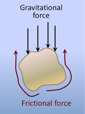
normal force (15) the component of the gravitational force that acts directly into the slope
North Atlantic Deep Water (18) deep Atlantic Ocean water that has descended in the far north of the basin in the area between Scandinavia and Greenland
nunatuk (16) a rocky peak that extends above the ice level of a continental glacier
O
obliquity (19) in the context of Milankovitch Cycles, the angle of the tilt of the Earth’s rotational axis with respect to the plane of its orbit around the Sun
ocean plain (18) the extremely flat surface of the deep ocean floor in areas unaffected by plate tectonic processes and volcanism
oil window (20) the depth range, which is approximately 2000 to 4000 m, within which the temperature is appropriate for the formation of oil from organic matter in sedimentary rock
ooid (6) a small (approximately 1 mm) sphere of calcite formed in areas of tropical shallow marine water with strong currents
olivine (2) a silicate mineral made up of isolated silica tetrahedra and with either iron or magnesium (or both) as the cations
Oort cloud (22) a spherical cloud of icy objects extending from between about 5,000 and 500,000 astronomical units (Sun-Earth distances) from the Sun (thought to be the source area of comets)
open-pit mine (20) a mine that is open to the surface
outcrop (5) a surface exposure of rock that is part of the crust (bedrock)
outwash plain (16) an extensive region of sand and gravel deposited by streams flowing out of a glacier (same as sandur)
overturned (12) a geological feature that has been tilted to the point where it is upside down
oxbow (13) a part of a stream meander that has become isolated from the rest of the stream as the result of a meander cutoff
oxidation (5) the reaction between a mineral and oxygen
oxide (2) a mineral in which the anion is oxygen (e.g., hematite Fe2O3)
P
pahoehoe (4) a lava flow with a ropy surface texture formed when the surface cools and hardens while the lava beneath is still flowing
paleomagnetic (10) past variations in the intensity and polarity of the Earth’s magnetic field
Pangea (10) the supercontinent that existed between approximately 300 and 180 Ma
paraconformity (8) an interruption representing a period of non-deposition, without tilting or erosion, in a sequence of sedimentary rocks
parasitic fold (12) a fold within a fold
parent rock (7) the rock that was already in existence when a process of metamorphism started
partial melting (3) the process during which a only specific mineral components of a rock melt in response to changing conditions
parting (6) a narrow gap between individual sedimentary layers
passive margin (10) a boundary between a continent and an ocean at which there is no tectonic activity (e.g., the eastern edge of North America)
paternoster lake (16) one of a series of rock basin lakes
pebble (6) a sedimentary particle ranging in size from 2 to 64 mm (includes granule)
pelagic (18) the part of a lake or the ocean that is not close to shore
permafrost (19) ground that remains frozen for two or more years
permanentism (10) the now discredited theory that the features on the Earth have not changed significantly over geological time
permeability (14) an expression of the ease with which liquid will flow through a porous medium
phaneritic (3) a rock texture in which the individual crystals or grains are visible to the naked eye
Phanerozoic (1) the most resent eon of geological time, encompassing the Paleozoic, Mesozoic and Cenozoic eras
phenocryst (3) a relatively large crystal within an igneous rock
phyllosilicate (2) a silicate mineral in which the silica tetrahedra are made up of sheets
phosphate (2) a mineral in which the anion is PO43-
photic zone (18) the upper 200 m of the ocean or a lake, where, depending on the turbidity of the water, light can penetrate
phreatic eruption (4) a steam-drive volcanic eruption that takes place when surface or near-surface water is heated by volcanic activity
phyllite (7) a metamorphic rock with slaty cleavage and a sheen on the surface produced by aligned micas
pillow (4) a pillow-shaped mass of volcanic rock (typically basalt) formed when magma erupts beneath the surface
pillow lava (4) a volcanic rock (typically basalt) that is made up primarily of pillows
pipe (3) a cylindrical body of igneous rock, typically resulting from a feeder conduit to a volcano
plate (1) a region of the lithosphere that is considered to be moving across the surface of the Earth as a single unit
plate tectonics (1) the concept that the Earth’s crust and upper mantle (lithosphere) is divided into a number of plates that move independently on the surface and interact with each other at their boundaries
plinian eruption (4) a large volcanic eruption in which a column of hot tephra and gases rises many kilometres into the atmosphere
pluton (3) a body of intrusive igneous rock
podsol (5) a soil with well-developed horizons formed in temperate forested regions
podsolization (5) the process of the formation of podsol
polar wandering path (10) a path of varying magnetic pole positions defined by paleomagnetic data (in fact it is now understood that the continents have wandered, not the poles, so a more appropriate terms is “apparent polar wandering path”)
polymerize (3) the formation of molecular chains within a fluid (e.g., a magma) that lead to an increase in the fluid’s viscosity
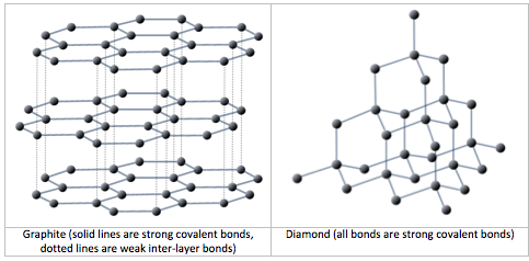
polymorphs (7) two or more minerals with the same chemical formula but different crystal structures
porosity (14) the percentage of open pore space within a body of rock or sediment
porphyritic (3) an igneous texture in which some of the crystals are distinctively larger than the rest
porphyry deposit (20) a mineral deposit (of copper or molybdenum especially) in which part of the host rock is a porphyritic stock
positive feedback (19) a process that results in an increase in that process (in the context of climate change it is a process that enhances the change in climate, such as the reduced reflectivity of the Earth’s surface when ice melts)
potassium feldspar (2) feldspar with the formula KAlSi3O8
potentiometric surface (14) the imaginary surface defined by the levels to which water would rise in a series of wells drilled into a confined aquifer
precession (19) in the context of Milankovitch Cycles, the variation in the direction at which the Earth’s rotational axis is pointing
principle of cross-cutting relationships (6) the principle that a body of rock that cuts across or through another body of rock is younger than that other body
principle of faunal succession (6) the principle that life on Earth has evolved in an orderly way, and that we can expect to always find fossils of a specific type in rocks of a specific age
principle of inclusions (6) the principle that inclusions within a body of rock must be older than the rock
principle of original horizontality (6) the principle that sedimentary beds are originally deposited in horizontal layers
principle of superposition (6) the principle that in a sequence of layered rocks that is not overturned or interrupted by faulting, the oldest will be at the bottom and the youngest at the top
proglacial (16) referring to the area in front of a glacier
proton (2) a sub-atomic particle with a mass of 1 and a charge of 1
protoplanetary disk (22) a rotating cloud of gas and dust surrounding a young star
pumice (4) a highly vesicular felsic volcanic rock (typically composed mostly of glass)
p-wave (9) a seismic body wave that is characterized by deformation of the rock in the same direction that the wave is propagating (compressional vibration)
pyroclastic (4) volcanic material formed during an explosive eruption
pyroclastic density current (4) a body of hot pyroclastic rock and gases that is flowing rapidly down the flank of a volcano
pyroxene (2) a single chain silicate mineral
Q
quartz (2) a silicate mineral with the formula SiO2
quartz sandstone (6) a sandstone in which more than 90% of the grains are quartz
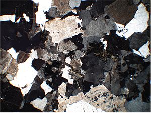
quartzite (7) a metamorphic rock formed from the contact or regional metamorphism of sandstone
R
radial (13) a pattern of streams radiating out from a central point, typically an isolated mountain
radioactivity (9) the natural transformation of unstable isotopes into new elements
radiolaria (18) microscopic (0.1 to 0.2 mm) marine protozoa that produce silica shells
Rayleigh wave (11) a surface seismic wave, with vertical motion
recharge (14) the transfer of surface water into the ground to become groundwater
recharge area (14) an area of an aquifer where recharge is predominant over discharge
rectangular drainage (13) a drainage pattern in which tributaries typically flow at right angles to each other and meet at right angles
recumbent fold (12) a fold that is overturned such that its limbs are close to horizontal
redshift (22) the increase in wavelength of light resulting from the fact that the source of the light is moving away from the observer
reef (17) a mound of carbonate formed in shallow tropical marine environments by corals, algae and a wide range of other organisms
regional metamorphism (7) metamorphism caused by burial of the parent rock to depths greater than 5 km (typically takes place beneath mountain ranges, and extends over areas of hundreds of km2)
remnant magnetism (10) magnetism of a body of rock that formed at the time the rock formed and is consistent with the magnetic field orientation that existed at that time and place
reservoir rock (20) rock into which petroleum has migrated and is now trapped
residual soil (5) soil formed by weathering of the underlying rock or sediment
retrograde metamorphism (7) metamorphism that takes place at a lower temperature than that at which the rock originally formed or was previously metamorphosed
reverse fault (12) a non-vertical fault along which the hanging wall (upper surface) has moved up relative to the footwall
rhyolite (3) a felsic volcanic rock
ridge push (10) the concept that at least part of the mechanism of plate motion is the push of oceanic lithosphere down from a ridge area
rip current (17) a strong flow of water outward from a beach
ripple (6) on a series of small parallel ridges formed within sediment that has accumulated in moving water or wind
rip-rap (17) angular rock fragments, typically boulder sized, used to armour slopes and shorelines against erosion
roche moutonée (16) a product of glaciation in which a bedrock protrusion is eroded into a streamlined shape that has a broken or jagged leading (down-ice) edge
rock avalanche (15) a rapid turbulent flow of broken bedrock fragments down a steep slope
rock basin lake (16) a lake situated in a rock basin carved at the upper end of an alpine glacier
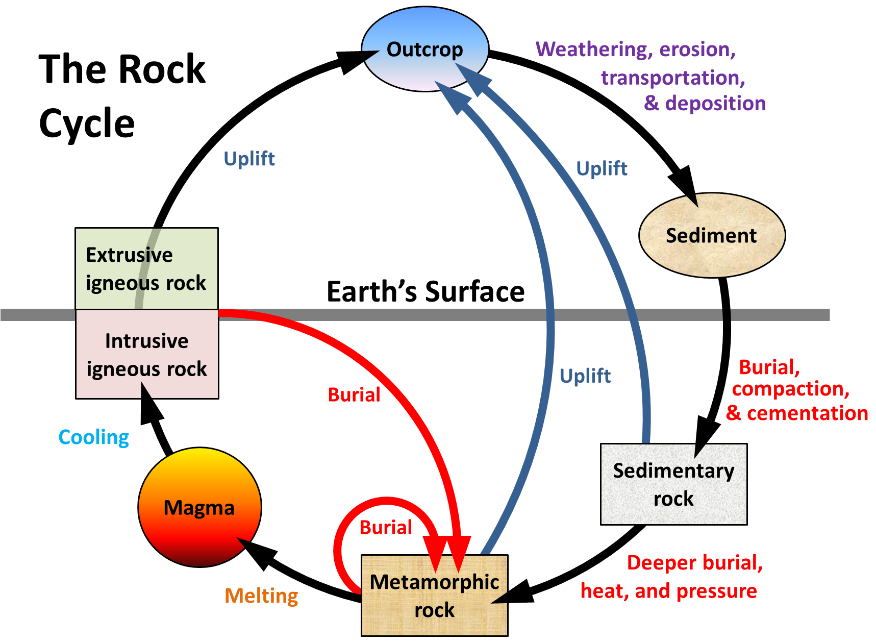
rock cycle (3) the series of processes through which rocks are transformed from one type to another
rock fall (15) the near-vertical fall or bouncing of rock released from a steep slope
rock slide (15) the translational motion of an essentially intact body of rock down a slope (rock slides are typically slow, because once they start to move fast the rock body becomes fragmented and then flows as a rock avalanche)
runoff (14) flow of water down a slope, either across the ground surface, or within a series of channels
rupture (11) breaking of rock subject to stress, typically resulting in an earthquake
rupture surface (11) the area over which rock rupture takes place during an earthquake
S
sackung (15) an escarpment or trough at the top of a slow-moving rock slide (sackungen)
salatation (13) the bouncing of particles along a stream bottom or desert floor
sand (6) a mineral or rock fragment ranging in size from 1/16th to 2 mm
sandstone (1) a rock that is primarily comprised of sand-sized particles
sandur (16) an extensive region of sand and gravel deposited by streams flowing out of a glacier (same as outwash plain)
saturated zone (14) the part of an aquifer, or any body of rock, that is saturated with water
schist (1) a metamorphic rock with visible aligned mica crystals
sea cave (17) a shallow cave formed on a rocky shore by wave erosion
sea cliff (17) a coastal escarpment that is typically eroding inland as a result of wave action
sea-floor spreading (10) the formation of new oceanic crust by volcanism at a divergent plate boundary
sector collapse (4) the sudden collapse of a significant part of the flank of a volcano
sedimentary rock (3) rock that has formed by the lithification of sediments
sediments (3) unconsolidated particles of mineral or rock
seismic (11) pertaining to earthquakes
seismic moment (11) a measurement of an earthquake’s energy based on longwave vibrations, or on the product of the fault area and displacement
seismic reflection sounding (10) measurement of the properties of sediments based on detection of sounds generated at surface and reflected from layers beneath the surface
septae (8) calcareous partitions between the successive living chambers in a cephalopod
septic system (14) a system constructed to facilitate the dispersion and detoxification of sewage (typically includes a septic tank and a drainage field)
shaft (20) a vertical opening at a mine
shale (6) a silt- and clay-rich rock that has evidence of layering
shear force (15) the component of the gravitational force in the direction parallel to a slope
shear strength (15) the strength of a body of rock or sediment that counteracts the shear force
shear stress (12) the stress placed on a body of rock or sediment adjacent to a fault
sheeted dykes (10) a series of near-vertical dykes formed in the vicinity of a spreading ridge when magma from depth flows into fractures formed by extensional forces
sheet silicate (2) a silicate mineral in which the silica tetrahedra are combined within sheets
sheetwash (5) overland flow of water, typically related to a heavy precipitation event
shield (4) a region of ancient (typically Precambrian) crystalline rock (equivalent to a craton)
shield volcano (4) a low-profile volcano formed primarily from eruptions of low-viscosity mafic magma
SIAL (sialic) (10) referring to rock or magma in which silica and aluminum are the predominant components (generally equivalent to felsic)
silica (2) a form of the mineral quartz (SiO2)
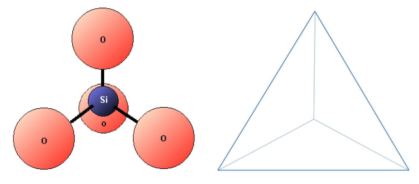
silica tetrahedron (2) a combination of 1 silicon atom and 4 oxygen atoms that form a tetrahedron
silicate (1) a mineral that includes silica tetrahedra
silicon (2) the 14th element
silicone (2) resin or caulking made from silicon-oxygen chains and various organic molecules
sill (3) an igneous intrusion that is parallel to existing layering in the country rock
silt (6) sedimentary particles ranging is size from 1/256th to 1/16th of a mm
SIMA (simatic) (10) referring to rock or magma in which silica, magnesium and iron are the predominant components (generally equivalent to mafic)
skarn (7) the contact metamorphism (and metasomatism) of limestone
slab pull (10) the concept that at least part of the mechanism of plate motion is the pull of oceanic lithosphere down into the mantle
slate (7) a fine-grained metamorphic rock that splits easily into sheets
slaty cleavage (7) the tendency for slate or phyllite to split into sheets (note that this is the only situation in this textbook where the term “cleavage” is applied to a rock as opposed to a mineral)
slide (15) the downward movement of rock or sediment on a slope as an intact mass
slump (15) a slide in which the nature of the motion is rotational (typically only develops in unconsolidated sediments)
smectite (2) a fine-grained sheet silicate mineral that can accept water molecules into interlayer spaces, resulting is swelling
smelter (20) a refinery at which minerals are processed to produce pure metals
snowline (22) in astronomy the radius around a star at which represents the boundary between gases (or liquids) and solids
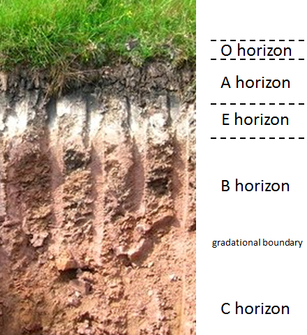
soil horizon (5) a layer, within a well-developed soil, that is physically or chemically different from layers above or below
solar system (22) a star and the planets surrounding it
solar wind (22) a stream of ionized (charged) particles away from the Sun
solid solution (2) the substitution of one element for another in a mineral (e.g., iron can be substituted for magnesium in the mineral olivine)
solifluction (15) the flow of water saturated sediment or soil over a stronger and less permeable substrate
source rock (20) the sedimentary rock from which petroleum originates prior to its migration into a reservoir rock
speleothem (6) a solutionally-formed feature within a limestone cave (e.g., a stalactite)
spit (17) a sand or coarser deposit extending from shore out into open water
spring (14) the flow of groundwater onto the surface
stack (17) a prominent rocky island that is a remnant of the erosion of a headland
stage (13) the level of water in a stream
stalactite (6) a cone-shaped speleothem that is suspended from the roof of a cave
stalagmite (6) a cone-shaped speleothem that forms on the floor of a cave
step-pool (13) a characteristic of stream flow in which water flows from one pool to another, typically on a stream with a steep gradient
stock (3) an irregular pluton with n exposed area less than 100 km2
stoping (3) the fracturing and incorporation of fragments of country rock as a magma body moves upward through the crust
strain (12) the deformation of rock that is subjected to stress
streak (2) the mark left on a porcelain plate when a mineral sample is ground to a powder by being rubbed across the plate (typically considered to provide a more reliable depiction of the colour than the whole sample)
stream (13) any body of flowing water
stress (12) a force applied to a rock
stress transfer (11) the change in the pattern of stress on a region of rock as a result of an earthquake (typically stress is reduced in the area of a rupture zone, but is increased elsewhere in the vicinity)
strike (12) the compass direction of a horizontal line on a sloped surface (e.g., bedding plane, fracture etc.)
strike-slip fault (12) a fault that is characterized by motion that is close to horizontal and parallel to the strike direction of the fault
subaerial eruption (4) a volcanic eruption that takes place on land
subaqueous eruption (4) a volcanic eruption that takes place under water
subducted (1) when part of a plate is forced beneath another plate along a subduction zone
subduction zone (10) the sloping region along which a tectonic plate descends into the mantle beneath another plate
subglacial (16) beneath a glacier
sulphate (2) a mineral in which the anion is SO42-
sulphide (2) a mineral in which the anion is S2-
supergroup (21) a stratigraphically-continuous series of related groups
superterrane (21) a number of terranes that are contiguous
supraglacial (16) on the surface of a glacier
surf zone (17) the near-shore zone where waves are breaking into surf
suture (8) the line on the surface of a cephalopod that marks the boundary between a septum and the outer shell
swash (17) the upward motion of a wave on a beach (typically takes place at the same angle that the waves are approaching the shore)
s-wave (9) a seismic body wave that is characterized by deformation of the rock transverse to the direction that the wave is propagating
symmetrical (12) a fold in which the limbs are at the same angle to the hinge
syncline (12) a downward fold where the beds are known not to be overturned
synform (12) a downward fold where it is not known if the beds are overturned
T
tailings (20) the fine-grained waste rock from a plant used to concentrate ore minerals
talus slope (15) a sloped deposit of angular rock fragments at the base of a rocky escarpment
tarn (16) a lake within a rock basin
tectonic plate (1) a region of the lithosphere that is considered to be moving across the surface of the Earth as a single unit
tectonic sea level change (17) relative sea level change related to the vertical motion of a crustal block caused by tectonic processes
tephra (4) fragments of volcanic rock (including volcanic ash) ejected during an explosive eruption
terminal moraine (16) and end moraine that marks the farthest forward advance of a glacier
terrane (7) a block of crust that has geological features that are distinctive from neighbouring regions, and is assumed to have been moved from elsewhere by tectonic processes
terrestrial planet (22) a planet with a rocky mantle and crust and metallic core (e.g., Earth)
terrigenous (18) referring to sedimentary particles that originated on a continent
test (6) the shell-like hard parts (either silica or carbonate) of small organisms such as radiolarian and foraminifera
thrust fault (11) a low angle reverse fault
till (16) unsorted sediment transported and deposited by glacial ice
tiltmeter (4) a sensitive instrument used to monitor subtle changes in the tilt of the land, particularly in studies of active volcanoes
tombolo (17) a sand or coarser deposit connecting an island or rocky prominence to a larger body of land
traction (13) a force that contributes to the movement of particles situated on a stream bed or desert floor
transform fault (10) a boundary between two plates that are moving horizontally with respect to each other
travertine (6) a deposit of calcium carbonate that forms at springs, hot springs or within limestone caves
trellis (13) a drainage pattern in which tributaries typically flow parallel to one other but meet at right angles
trigger (15) an event, such as an earthquake or a heavy rainfall, that triggers the onset of a mass wasting event
trough (17) the lowest point of a wave
truncated spur (16) the steep end of a ridge or arête that has been eroded by a main-valley glacier
tsunami (11) a long-wavelength wave produced by the vertical motion of the floor of the ocean or a large lake, typically related either to an earthquake or a sub-marine mass wasting event
tufa (6) a form of travertine that is especially porous as it forms around existing vegetative material.
tuya (4) a flat-topped volcanic hill or mountain that formed when an eruption took place beneath a glacier and the melting led to the formation of a lake that then resulted in the wave-erosion of the top of the volcano
U
unconfined aquifer (14) an aquifer that is not overlain by a confining layer
unconformity (8) a geological boundary at the base of a sedimentary layer
unconformity-type uranium deposit (20) a uranium deposit that has formed at a nonconformity between sandstone and older rock
uncompressed density (22) the density of planetary material that it would have it was not compressed by the planets gravitational force
underground storage tank (14) (UST) an underground tank for storing liquids, most commonly for liquid fuel
unsaturated zone (14) the rock or sediment above the water table
U-shaped valley (16) a relatively straight valley with a flat bottom and steep sides that has been carved by a valley glacier
V
valley glacier (16) a glacier formed in a mountainous region and confined to a valley (same as alpine glacier)
varve (16) a recognizable layer within sediments that represents a single year of deposition
vesicular (3) an igneous texture characterized by holes left by gas bubbles
volcanic glass (2) magma that has cooled within minutes, not allowing time for the formation of crystals
volcanic-hosted massive sulphide (20) a mineral deposit hosted by volcanic rocks and including zones where most of the rock is made up of sulphide minerals (including ore minerals and pyrite)
W
wacke (6) a sandstone with more than 15% clay and silt
water table (14) the upper surface of the saturated zone in an unconfined aquifer
wave base (17) the depth of water that is affected by the sub-surface orbital motion of wave action (approximately one-half of the wavelength)
wave-cut platform (17) a nearly-horizontal bench of rock eroded by waves within the surf zone (equivalent to wave-cut terrace)
wavelength (17) the distance between the crests of two waves
weathering (5) a range of processes taking place in the surface environment, through which solid rock is transformed into sediment and ions in solution
Western Canada Sedimentary Basin (21) a large basin in the western interior of Canada, east of the Rocky Mountains, extending from the northern United States to the Northwest Territories
Wisconsin Glaciation (16) the most recent advance of the Pleistocene glaciations, extending from 85 to 11 ka
X
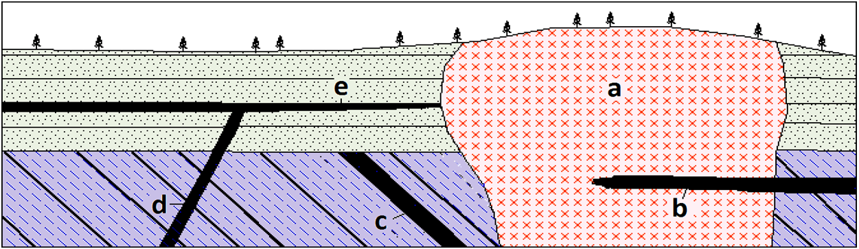
xenolith (3) a fragment of country incorporated into igneous rock, commonly as a result of stoping
Y
youthful stream (13) a stream that is actively down-cutting its valley in an area that has recently been uplifted
Z
zone of ablation (16) the part of a glacier, below the equilibrium line, where there is net loss of ice mass due to melting and calving
zone of accumulation (16) the part of a glacier, above the equilibrium line, where there is net gain of ice mass because not all of the snow that falls each winter is able to melt during the following summer

![Photograph of Rearguard Mt. and Robson Glacier in the Rocky Mountains of British Columbia [SE]](http://opentextbc.ca/geology/wp-content/uploads/sites/110/2015/08/Rearguard-Mt.-and-Robson-Glacier.jpg)
![Photograph of the aftermath of a deadly debris flow in the Riverside Drive area of North Vancouver in January, 2005 [The Province, used with permission]](http://opentextbc.ca/geology/wp-content/uploads/sites/110/2015/08/deadly-debris-flow-in-the-Riverside-Drive.jpg)
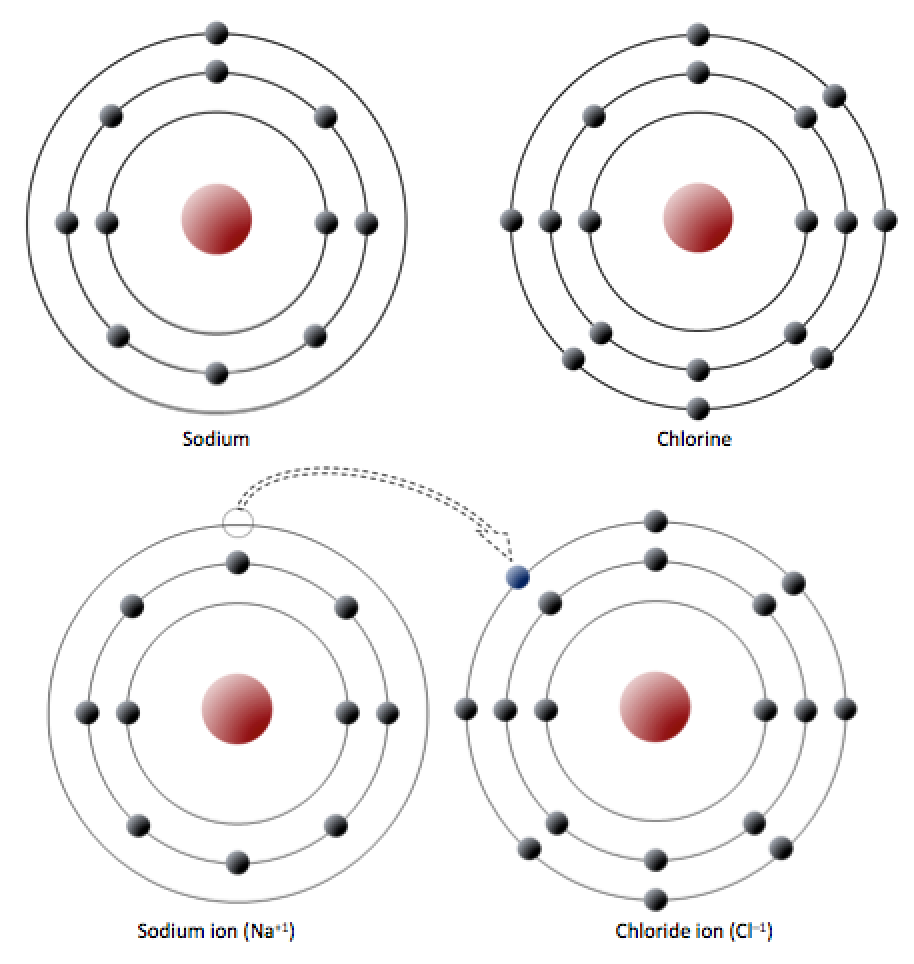
![Figure 1.4 The lattice structure and composition of the mineral halite (common table salt) [SE]](http://opentextbc.ca/geology/wp-content/uploads/sites/110/2015/08/lattice-structure-and-composition-of-the-mineral-halite.png)
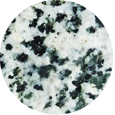
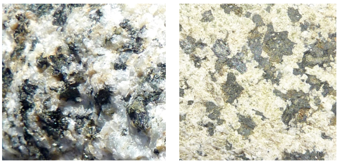
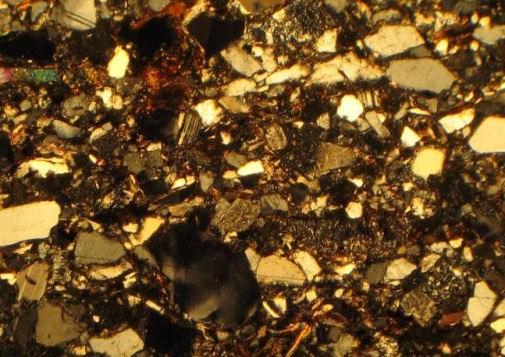
![Figure 1.5 A close-up view of the rock granite and some of the minerals that it typically contains (H = hornblende (amphibole), Q = quartz and F = feldspar). The crystals range from about 0.1 to 3 mm in diameter. Most are irregular in outline, but some are rectangular. [SE]](http://opentextbc.ca/geology/wp-content/uploads/sites/110/2015/08/close-up-view-of-the-rock-granite.png)
![The structure of the Earth’s interior showing the inner and outer core, the different layers of the mantle, and the crust [Wikipedia]](http://opentextbc.ca/geology/wp-content/uploads/sites/110/2015/08/structure-of-the-Earth’s-interior.png)
![A model of convection within the Earth’s mantle [http://upload.wikimedia.org/wikipedia/commons/thumb/2/27/Oceanic_spreading.svg/1280px-Oceanic_spreading.svg.png]](http://opentextbc.ca/geology/wp-content/uploads/sites/110/2015/08/convection-within-the-Earth’s-mantle.png)
![Figure 1.8 Earth’s tectonic plates and tectonic features that have been active over the past 1 million years [http://commons.wikimedia.org/wiki/File:Plate_tectonics_map.gif]](https://opentextbc.ca/physicalgeologyearle/wp-content/uploads/sites/145/2016/03/Plate-tectonics-map-2.gif)


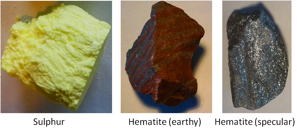
![Figure 2.17 The streak colours of earthy hematite (left) and specular hematite (right). Although the specular hematite streak looks close to black, it does have red undertones that you can see if you look closely. [SE]](https://opentextbc.ca/physicalgeologyearle/wp-content/uploads/sites/145/2016/06/hem-1.jpg)

![Figure 3.1 A fine-grained mafic dyke (dark green) intruded into a felsic dyke (pink) and into coarse diorite (grey), Quadra Island, B.C. All of these rocks are composed of more than one type of mineral. The mineral components are clearly visible in the diorite, but not in the other two rock types. [SE photo]](https://opentextbc.ca/physicalgeologyearle/wp-content/uploads/sites/145/2016/06/dyke2.jpg)
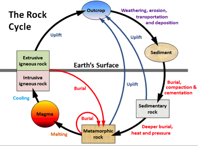
![Figure 3.2 A schematic view of the rock cycle. [SE]](https://opentextbc.ca/physicalgeologyearle/wp-content/uploads/sites/145/2016/06/rock-cycle2.png)
![Figure 3.3 Magma forming pahoehoe basalt at Kilauea Volcano, Hawaii [SE]](https://opentextbc.ca/physicalgeologyearle/wp-content/uploads/sites/145/2016/06/magma2.jpg)
![Figure 3.4 Cretaceous-aged marine sandstone overlying mudstone, Gabriola Island, B.C. [SE]](https://opentextbc.ca/physicalgeologyearle/wp-content/uploads/sites/145/2016/06/marine-sandstone2.jpg)
![Figure 3.5 Metamorphosed and folded Triassic-aged limestone, Quadra Island, B.C. [SE]](https://opentextbc.ca/physicalgeologyearle/wp-content/uploads/sites/145/2016/06/limestone2.jpg)
![Figure 3.6 Average elemental proportions in Earth’s crust, which is close to the average composition of magmas within the crust [SE]](https://opentextbc.ca/physicalgeologyearle/wp-content/uploads/sites/145/2016/06/earths-crust2.png)
![Figure 3.8 Mechanisms for (a) decompression melting (the rock is moved toward the surface) and (b) flux melting (water is added to the rock) and the melting curve is displaced. [SE]](https://opentextbc.ca/physicalgeologyearle/wp-content/uploads/sites/145/2016/06/flux-decompression.png)
![Figure 3.9 Common sites of magma formation in the upper mantle. The black circles are regions of partial melting. The blue arrows represent water being transferred from the subducting plates into the overlying mantle. [SE, after USGS (http://pubs.usgs.gov/gip/dynamic/Vigil.html)]](https://opentextbc.ca/physicalgeologyearle/wp-content/uploads/sites/145/2016/06/magma-formation2.png)
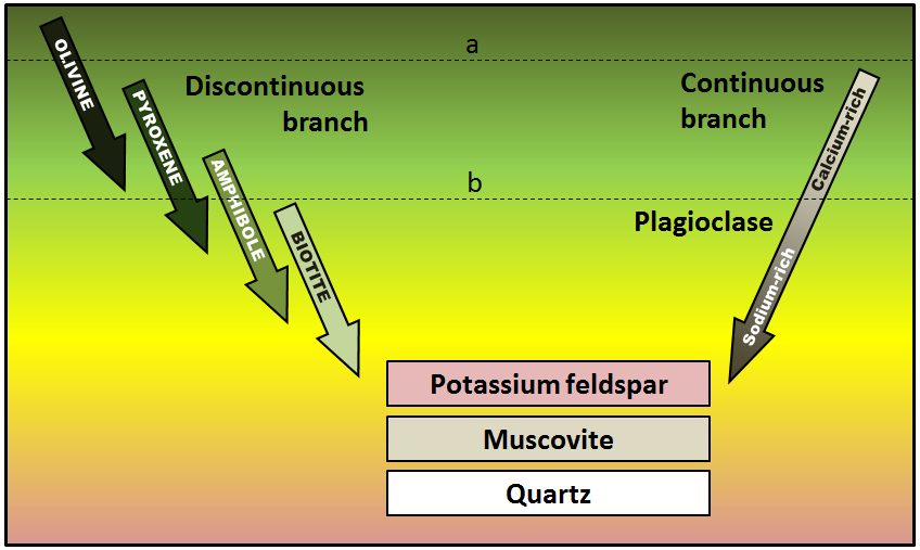
![Figure 3.10 The Bowen reaction series describes the process of magma crystallization [SE]](https://opentextbc.ca/physicalgeologyearle/wp-content/uploads/sites/145/2016/06/Bowen-reaction2.png)
![Figure 3.12 The chemical compositions of typical mafic, intermediate, and felsic magmas and the types of rocks that form from them. [SE]](https://opentextbc.ca/physicalgeologyearle/wp-content/uploads/sites/145/2016/06/mafic2.png)
![Figure 3.13 Examples of the igneous rocks that form from mafic, intermediate, and felsic magmas. [SE]](https://opentextbc.ca/physicalgeologyearle/wp-content/uploads/sites/145/2016/06/igneous-rocks2.png)
![Figure 3.14 An example of crystal settling and the formation of a zoned magma chamber [SE]](https://opentextbc.ca/physicalgeologyearle/wp-content/uploads/sites/145/2016/06/magma-chamber2.png)
![Figure 3.15 Porphyritic textures: volcanic porphyry (left – olivine crystals in Hawaiian basalt) and intrusive porphyry (right) [SE]](https://opentextbc.ca/physicalgeologyearle/wp-content/uploads/sites/145/2016/06/porphyry.png)
![Figure 3.16 A simplified classification diagram for igneous rocks based on their mineral compositions [SE]](https://opentextbc.ca/physicalgeologyearle/wp-content/uploads/sites/145/2016/06/ingeous-rocks2.png)
![Figure 3.18 A pegmatite with mica, quartz, and tourmaline (black) from the White Elephant mine, South Dakota [from http://en.wikipedia.org/wiki/Pegmatite#mediaviewer/File:We-pegmatite.jpg]](https://opentextbc.ca/physicalgeologyearle/wp-content/uploads/sites/145/2016/06/pegmatite2.jpg)
![Figure 3.19 Xenoliths of mafic rock in granite, Victoria, B.C. The fragments of dark rock have been broken off and incorporated into the light-coloured granite. [SE]](https://opentextbc.ca/physicalgeologyearle/wp-content/uploads/sites/145/2016/06/xenoliths2.jpg)
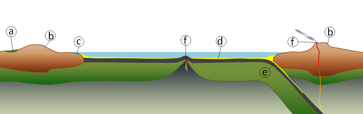
![Figure 3.20 Depiction of some of the types of plutons. a: stocks (if they coalesce at depth then they might constitute a batholith), b: sill (a tabular body, in this case parallel to bedding), c: dyke (cross-cuts bedding), d: laccolith (a sill that has pushed up the overlying rock layers), e: pipe (a cylindrical conduit feeding a volcano). The two features labelled f could be pipes or dykes, but from this perspective it’s not possible to determine if they are cylindrical or tabular. [SE drawing]](http://opentextbc.ca/geology/wp-content/uploads/sites/110/2015/09/igneous-intrusives-4.png)
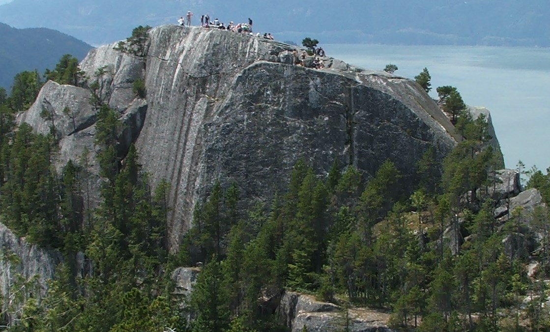
![Figure 3.21 The Stawamus Chief, part of the Coast Range Plutonic Complex, near to Squamish, B.C. The cliff is about 600 m high. Most of the dark stripes are a result of algae and lichen growth where the surface is frequently wet, but there is a large (about 10 m across) vertical dyke that extends from bottom to top. [SE photo]](https://opentextbc.ca/physicalgeologyearle/wp-content/uploads/sites/145/2016/06/stawamus-chief2.jpg)
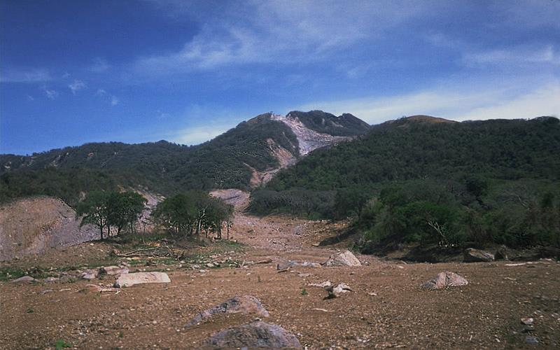
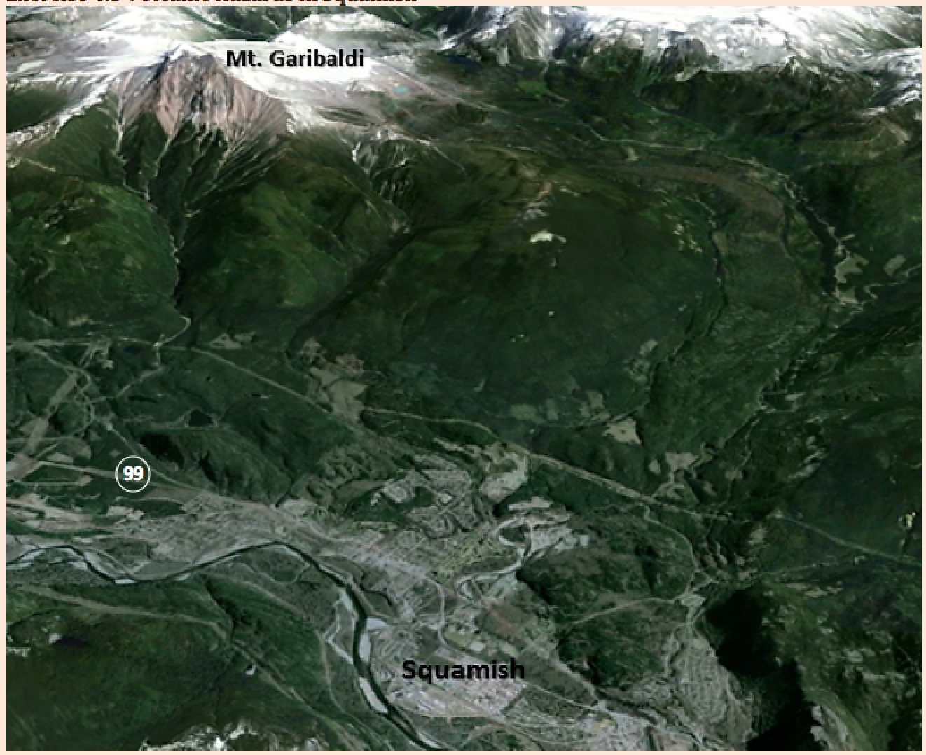
![Figure 4.1 Mt. Garibaldi, near Squamish B.C., is one of Canada’s tallest (2,678 m) and most recently active volcanoes. It last erupted approximately 10,000 years ago. [SE photo]](https://opentextbc.ca/physicalgeologyearle/wp-content/uploads/sites/145/2016/06/garibaldi-1.jpg)
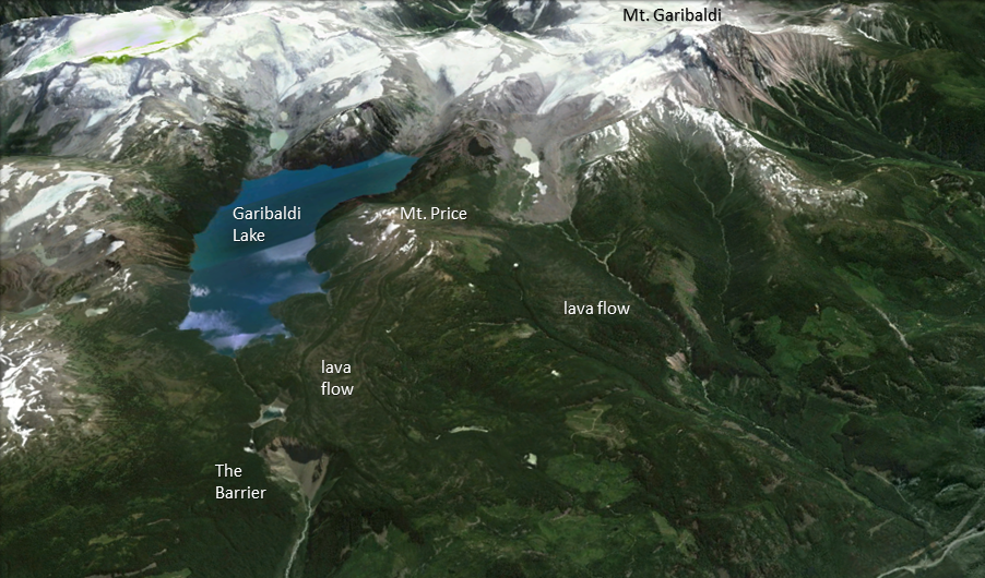
![Figure 4.2 Mt. Garibaldi (background left, looking from the north) with Garibaldi Lake in the foreground. The volcanic peak in the centre is Mt. Price and the dark flat–topped peak is The Table. All three of these volcanoes were active during the last glaciation. [SE photo]](https://opentextbc.ca/physicalgeologyearle/wp-content/uploads/sites/145/2016/06/garibaldi-2.jpg)
![Figure 4.3 The plate-tectonic settings of common types of volcanism. Composite volcanoes form at subduction zones, either on ocean-ocean convergent boundaries (left) or ocean-continent convergent boundaries (right). Both shield volcanoes and cinder cones form in areas of continental rifting. Shield volcanoes form above mantle plumes, but can also form at other tectonic settings. Sea-floor volcanism can take place at divergent boundaries, mantle plumes and ocean-ocean-convergent boundaries. [SE, after USGS (http://pubs.usgs.gov/gip/dynamic/Vigil.html)]](https://opentextbc.ca/physicalgeologyearle/wp-content/uploads/sites/145/2016/06/volcanic-tectonics.png)
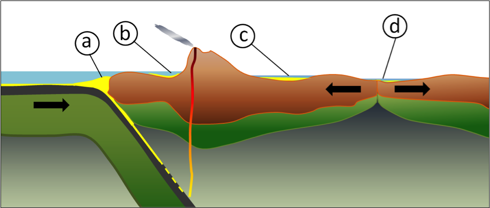
![Figure 4.4 The processes that lead to volcanism in the three main volcanic settings on Earth: (a) volcanism related to plate divergence, (b) volcanism at an ocean-continent boundary*, and (c) volcanism related to a mantle plume. [SE, after USGS (http://pubs.usgs.gov/gip/dynamic/Vigil.html)] *Similar processes take place at an ocean-ocean convergent boundary.](https://opentextbc.ca/physicalgeologyearle/wp-content/uploads/sites/145/2016/06/volcanic-tectonics-2.png)
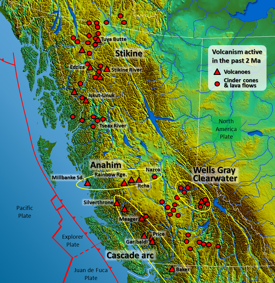
![Figure 4.5 Volcanoes and volcanic fields in the Northern Cordillera Volcanic Province, B.C. (base map from Wikipedia (http://commons.wikimedia.org/wiki/File:South-West_Canada.jpg). Volcanic locations from Edwards, B. & Russell, J. (2000). Distribution, nature, and origin of Neogene-Quaternary magmatism in the northern Cordilleran volcanic province, Canada. Geological Society of America Bulletin. pp. 1280-1293[SE]Cordillera Volcanic Province, B.C.](https://opentextbc.ca/physicalgeologyearle/wp-content/uploads/sites/145/2016/06/stikine.png)
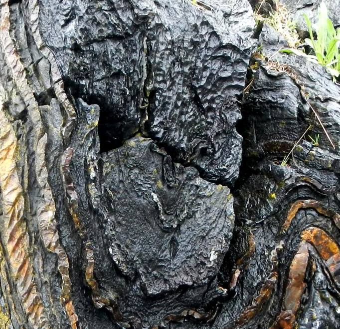
![Figure 4.6 Volcanic rock at the Tseax River area, northwestern B.C. [SE]](https://opentextbc.ca/physicalgeologyearle/wp-content/uploads/sites/145/2016/06/tseax.jpg)

![Figure 4.11 The north side of Mt. St. Helens in southwestern Washington State, 2003 [SE photo]. The large 1980 eruption reduced the height of the volcano by 400 m, and a sector collapse removed a large part of the northern flank. Between 1980 and 1986 the slow eruption of more mafic and less viscous lava led to construction of a dome inside the crater.](https://opentextbc.ca/physicalgeologyearle/wp-content/uploads/sites/145/2016/03/msh-3.jpg)
![Figure 4.13 Mt. St. Helens volcanic deposits: (a) lahar deposits (L) and felsic pyroclastic deposits (P) and (b) a columnar basalt lava flow. The two photos were taken at locations only about 500 m apart. [SE]](https://opentextbc.ca/physicalgeologyearle/wp-content/uploads/sites/145/2016/06/msh-3.png)
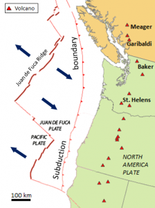 The map shown here illustrates the interactions between the North America, Juan de Fuca, and Pacific Plates off the west coast of Canada and the United States. The Juan de Fuca Plate is forming along the Juan de Fuca ridge, and is then subducted beneath the North America Plate along the red line with teeth on it (“Subduction boundary”).
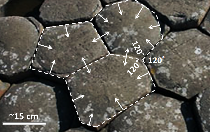

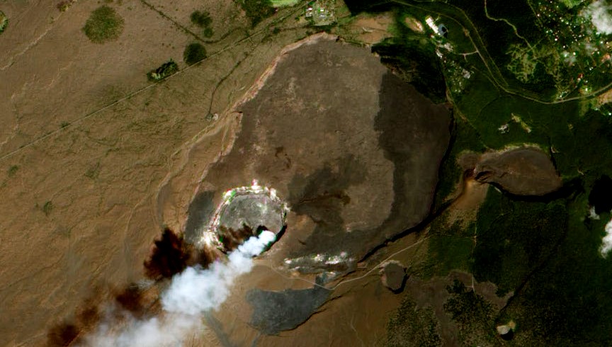
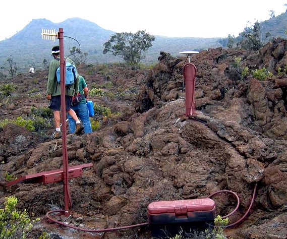
![Figure 4.17 A gas-composition monitoring station (left) within the Kilauea caldera and at the edge of Halema’uma’u crater. The rising clouds are mostly composed of water vapour, but also include carbon dioxide and sulphur dioxide. Sulphur crystals (right) have formed around a gas vent in the caldera. [SE photos]](https://opentextbc.ca/physicalgeologyearle/wp-content/uploads/sites/145/2016/06/kilauea-monitor.png)
![Figure 4.19 Images of Kilauea volcano taken in 2002 (b & c) and 2007 (a & d) [SE photos] (a) Pu'u'O'o cinder cone in the background with tephra in the foreground and aa lava in the middle, (b) Formation of pahoehoe on the southern edge of Kilauea, (c) Formation of aa on a steep slope on Kilauea, (d) Skylight in an active lava tube, Kilauea.](https://opentextbc.ca/physicalgeologyearle/wp-content/uploads/sites/145/2016/06/kilauea-lavas.png)
![Figure 4.20 A part of the Columbia River Basalt Group at Frenchman Coulee, eastern Washington. All of the flows visible here have formed large (up to two metres in diameter) columnar basalts, a result of relatively slow cooling of flows that are tens of m thick. The inset map shows the approximate extent of the 17 to 14 Ma Columbia River Basalts, with the location of the photo shown as a star. [SE – photo and drawing]](https://opentextbc.ca/physicalgeologyearle/wp-content/uploads/sites/145/2016/06/columbia.png)
![Figure 4.21 Modern and ancient sea-floor pillow basalts (left) Modern sea-floor pillows in the south Pacific [NOAA, from http://en.wikipedia.org/wiki/ Basalt#mediaviewer/File:Pillow_basalt_crop_l.jpg] (right) Eroded 40 to 50 Ma pillows on the shore of Vancouver Island, near to Sooke. The pillows are 30 to 40 cm in diameter. [SE]](https://opentextbc.ca/physicalgeologyearle/wp-content/uploads/sites/145/2016/06/pillows.png)
![Figure 4.22 Ekati diamond mine, Northwest Territories, part of the Lac de Gras kimberlite field [http://upload.wikimedia.org/wikipedia/commons/8/88/Ekati_mine_640px.jpg]](https://opentextbc.ca/physicalgeologyearle/wp-content/uploads/sites/145/2016/06/ekati.png)


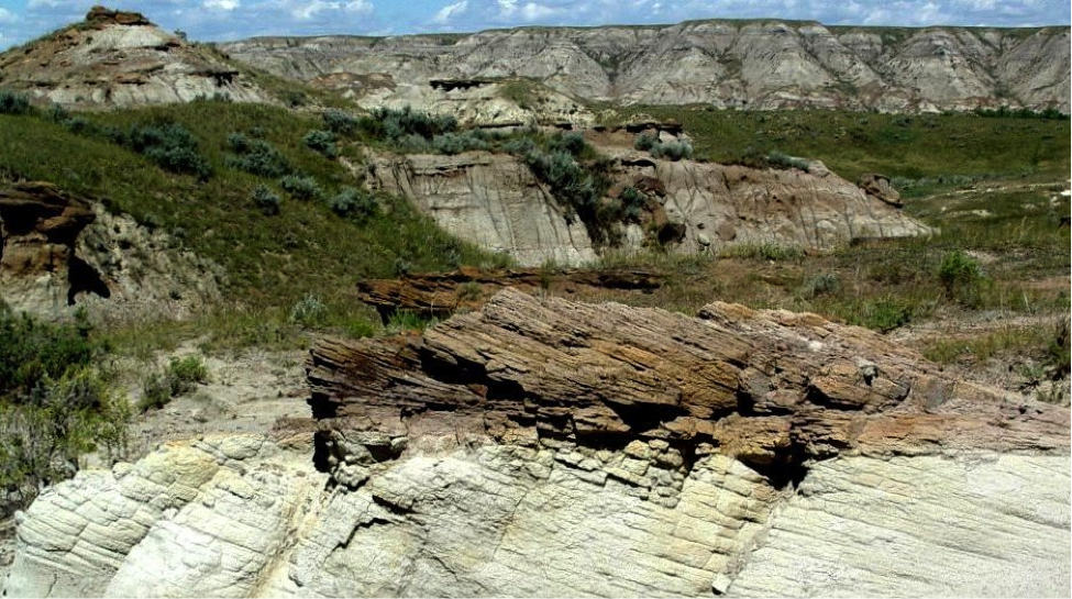
![Figure 5.1 The Hoodoos, near Drumheller, Alberta, have formed from the differential weathering of sedimentary rock that was buried beneath other rock for close to 100 Ma [SE photo]](https://opentextbc.ca/physicalgeologyearle/wp-content/uploads/sites/145/2016/03/hoodoos-2.jpg)
![Figure 5.4 Exfoliation of slate at a road cut in the Columbia Mountains west of Golden, B.C. [SE photo]](https://opentextbc.ca/physicalgeologyearle/wp-content/uploads/sites/145/2016/03/slate-2.jpg)


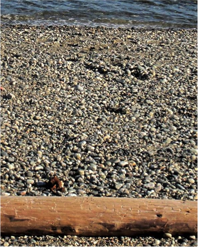
![Figure 5.13 Products of weathering and erosion formed under different conditions. [SE]](https://opentextbc.ca/physicalgeologyearle/wp-content/uploads/sites/145/2016/03/clasts-3.png)


![Figure 6.24 Mudcracks in volcanic mud at a hot-spring area near Myvatn, Iceland [SE]](https://opentextbc.ca/physicalgeologyearle/wp-content/uploads/sites/145/2016/06/myvatn-mudcracks.jpg)

![Figure 7.2 The rock cycle. The processes related to metamorphic rocks are at the bottom of the cycle. [SE ]](http://opentextbc.ca/geology/wp-content/uploads/sites/110/2015/07/image0021.png)
![Figure 7.3 The temperature and pressure stability fields of the three polymorphs of Al2SiO5. (Pressure is equivalent to depth. Kyanite is stable at low to moderate temperatures and low to high pressures, andalusite at moderate temperatures and low pressures, and sillimanite is stable at higher temperatures.) [SE]](http://opentextbc.ca/geology/wp-content/uploads/sites/110/2015/07/image0031.png)
![Figure 7.4 An illustration of different types of pressure on rocks. (a) confining pressure, where the pressure is essentially equal in all directions, (b) directed pressure, where the pressure form the sides is greater than that from the top and bottom, and (c) sheer stress caused by different blocks of rock being pushed in different directions. (In a and b there is also pressure in and out of the page.) [SE]](http://opentextbc.ca/geology/wp-content/uploads/sites/110/2015/07/image004.png)
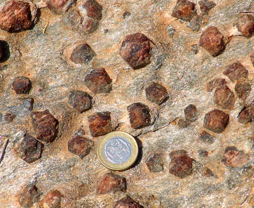 This photo shows a sample of garnet-mica schist from the Greek island of Syros. The large reddish crystals are garnet, and the surrounding light coloured rock is dominated by muscovite mica. The Euro coin is 23 mm in diameter. Assume that the diameters of the garnets increased at a rate of 1 mm per million years.
![Figure 7.5 The textural effects of squeezing during metamorphism. [SE]](http://opentextbc.ca/geology/wp-content/uploads/sites/110/2015/07/image006.png)
![Figure 7.6 The textural effects of squeezing and aligned mineral growth during metamorphism. The left-hand diagram represents shale with bedding in the direction shown. The right-hand diagram represents schist (derived from that shale), with the mica crystals orientated perpendicular to the main stress direction and the original bedding no longer easily visible. [SE]](http://opentextbc.ca/geology/wp-content/uploads/sites/110/2015/07/image007.png)
![Figure 7.7 A slate boulder on the side of Mt. Wapta in the Rockies near Field, BC. Bedding is visible as light and dark bands sloping steeply to the right (white arrow). Slaty cleavage is evident from the way the rock has broken and also from lines of weakness that same trend (yellow arrows). [SE]](http://opentextbc.ca/geology/wp-content/uploads/sites/110/2015/07/image008.jpg)
![Figure 7.8 Examples of foliated metamorphic rocks [a, b, and d: SE, c: Michael C. Rygel, http://en.wikipedia.org/wiki/Schist#mediaviewer/File:Schist_detail.jpg]](https://opentextbc.ca/physicalgeologyearle/wp-content/uploads/sites/145/2016/03/foliated-textures-2.png)
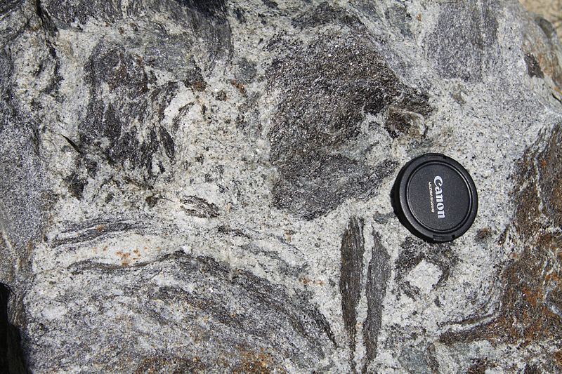
![Figure 7.10 Marble with visible calcite crystals (left) and an outcrop of banded marble (right) [SE (left) and http://gallery.usgs.gov/images/08_11_2010/a1Uh83Jww6_08_11_2010/large/DSCN2868.JPG (right)]](http://opentextbc.ca/geology/wp-content/uploads/sites/110/2015/07/Marble-.png)
![Figure 7.11 Quartzite from the Rocky Mountains, found in the Bow River at Cochrane, Alberta [SE]](http://opentextbc.ca/geology/wp-content/uploads/sites/110/2015/07/image016.jpg)
![Figure 7.12 Magnified thin section of quartzite in polarized light. The irregular-shaped white, grey, and black crystals are all quartz. The small, thin brightly-coloured crystals, are mica. This rock is foliated, even though it might not appear to be if examined without a microscope, and so it must have formed under directed-pressure conditions. [Photo by Sandra Johnstone, used with permission]](http://opentextbc.ca/geology/wp-content/uploads/sites/110/2015/07/image017.png)
![Figure 7.13 Hornfels from the Novosibirsk region of Russia. The dark and light bands are bedding. The rock has been recrystallized during contact metamorphism and does not display foliation. (scale in cm) [http://en.wikipedia.org/wiki/Hornfels#mediaviewer/ File:Hornfels.jpg]](http://opentextbc.ca/geology/wp-content/uploads/sites/110/2015/07/image018.jpg)
![Figure 7.14 Environments of metamorphism in the context of plate tectonics: a) regional metamorphism related to mountain building at a continent-continent convergent boundary, b) regional metamorphism of oceanic crust in the area on either side of a spreading ridge, c) regional metamorphism of oceanic crustal rocks within a subduction zone, d) contact metamorphism adjacent to a magma body at a high level in the crust, and e) regional metamorphism related to mountain building at a convergent boundary. [SE]](http://opentextbc.ca/geology/wp-content/uploads/sites/110/2015/07/image019.png)
![Figure 7.15 a: Regional metamorphism beneath a mountain range related to continent-continent collision (typical geothermal gradient). (Example: Himalayan Range) [SE]](http://opentextbc.ca/geology/wp-content/uploads/sites/110/2015/07/image020.png)
![Figure 7.16 b: Regional metamorphism of oceanic crustal rock on either side of a spreading ridge. (Example: Juan de Fuca spreading ridge) [SE]](http://opentextbc.ca/geology/wp-content/uploads/sites/110/2015/07/image021.png)
![Figure 7.17 c: Regional metamorphism of oceanic crust at a subduction zone. (Example: Cascadia subduction zone. Rock of this type is exposed in the San Francisco area.) [SE]](http://opentextbc.ca/geology/wp-content/uploads/sites/110/2015/07/image022.png)
![Figure 7.18 Franciscan Complex blueschist rock exposed north of San Francisco. The blue colour of rock is due to the presence of the amphibole mineral glaucophane. [SE]](https://opentextbc.ca/physicalgeologyearle/wp-content/uploads/sites/145/2016/03/franciscan-2.png)
![Figure 7.19 d: Contact metamorphism around a high-level crustal magma chamber. (Example: the magma chamber beneath Mt. St. Helens.) e: Regional metamorphism in a volcanic-arc related mountain range. (volcanic-region temperature gradient) (Example: The southern part of the Coast Range, BC.) [SE]](http://opentextbc.ca/geology/wp-content/uploads/sites/110/2015/07/image025.png)
![Figure 7.20 Types of metamorphism shown in the context of depth and temperature under different conditions. The metamorphic rocks formed from mudrock under regional metamorphosis with a typical geothermal gradient are listed. The letters a through e correspond with those shown in Figures 7.14 to 7.17 and 7.19. [SE]](https://opentextbc.ca/physicalgeologyearle/wp-content/uploads/sites/145/2016/03/depth-temp.png)
![Figure 7.21 Metamorphic index minerals and their approximate temperature ranges [SE]](http://opentextbc.ca/geology/wp-content/uploads/sites/110/2015/07/image027.png)
![Figure 7.22 Regional metamorphic zones in the Meguma Terrane of southwestern Nova Scotia [SE, after Keppie, D, and Muecke, G, 1979, Metamorphic map of Nova Scotia, N.S. Dept. of Mines and Energy, Map 1979-006., and from White, C and Barr, S., 2012, Meguma Terrane revisted, Stratigraphy, metamorphism, paleontology and provenance, Geoscience Canada, V. 39, No.1]](https://opentextbc.ca/physicalgeologyearle/wp-content/uploads/sites/145/2016/03/meguma-map-2.png)
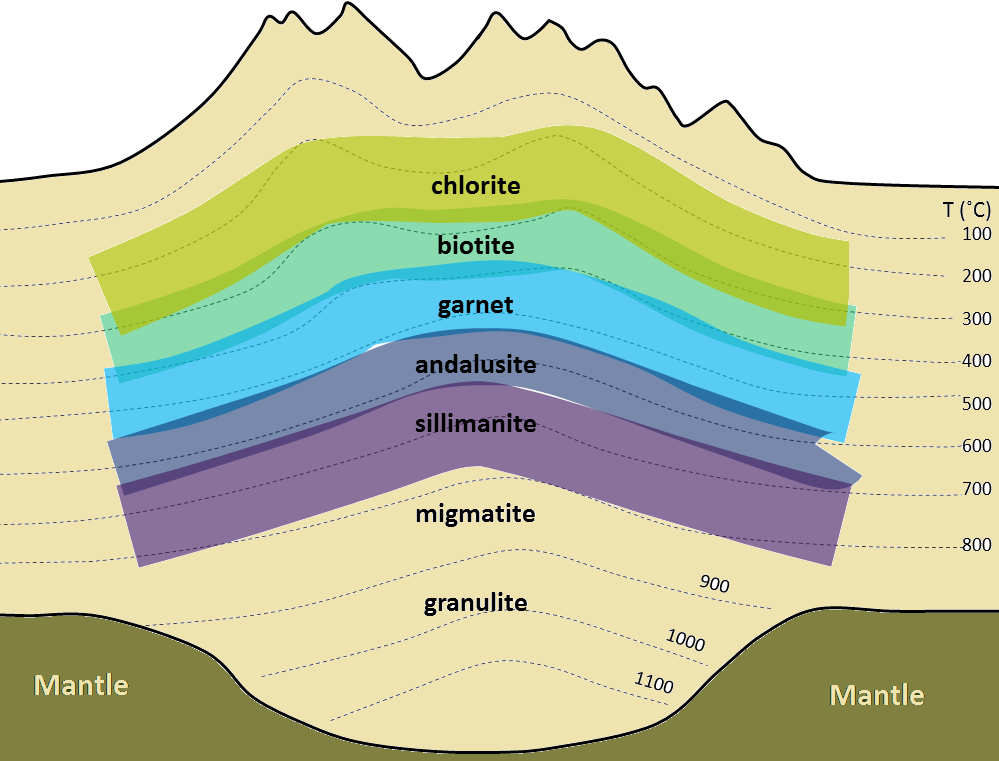
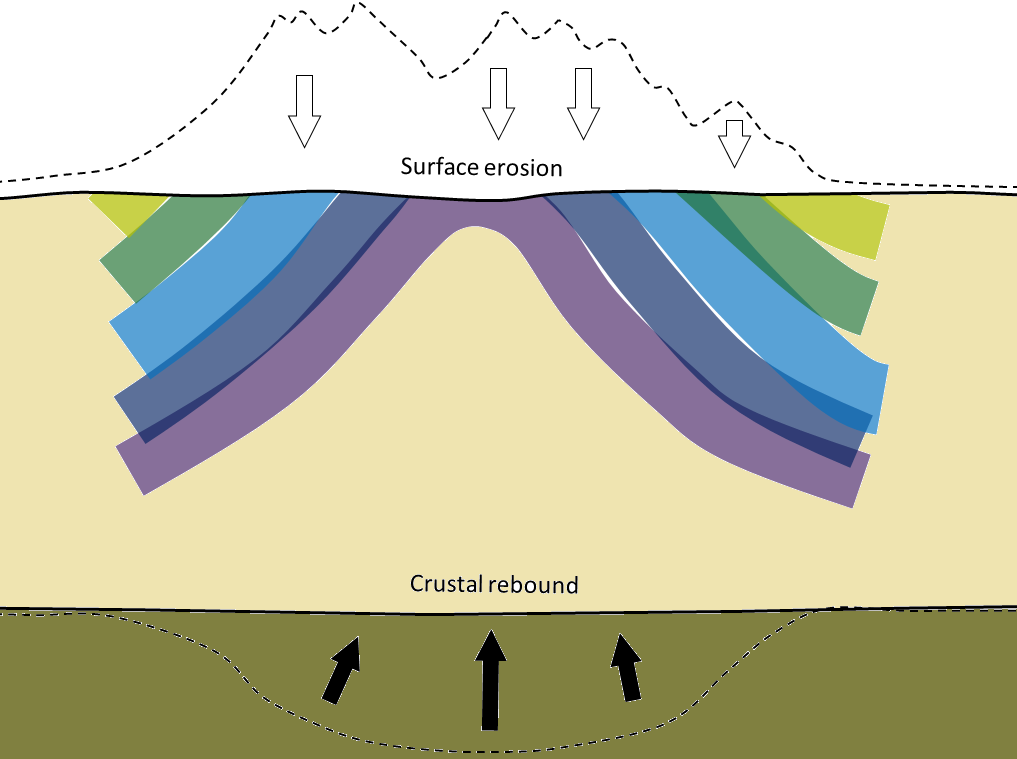
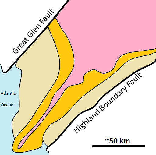
![Figure 7.24 Schematic cross-section of the middle and upper crust showing two magma bodies. The upper body, which has intruded into cool unmetamorphosed rock, has created a zone of contact metamorphism. The lower body is surrounded by rock that is already hot (and probably already metamorphosed), and so it does not have a significant metamorphic aureole. [SE]](http://opentextbc.ca/geology/wp-content/uploads/sites/110/2015/07/image032.png)
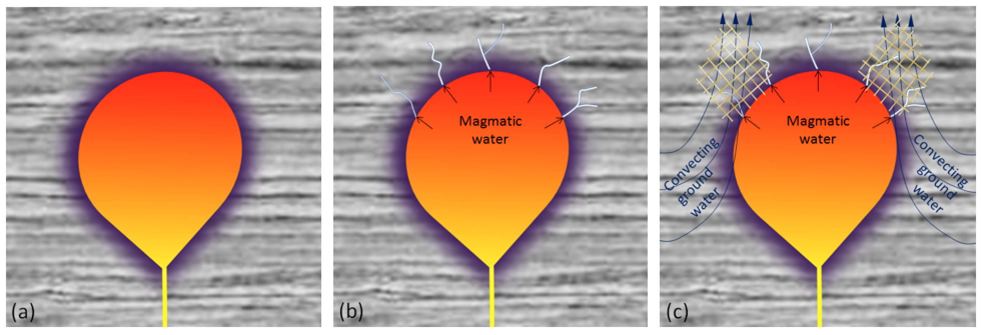
![Figure 7.26 Calcite veins in limestone of the Comox Formation, Nanaimo, B.C. [SE]](https://opentextbc.ca/physicalgeologyearle/wp-content/uploads/sites/145/2016/03/calcite-vein-2.jpg)
![Figure 7.27 A skarn rock from Mount Monzoni, Northern Italy, with recrystallized calcite (blue) garnet (brown) and pyroxene (green). The rock is 6 cm across. [by Siim Sepp, from http://commons.wikimedia.org/wiki/File:00031_6_cm_grossular_calcite_augite_skarn.jpg]](http://opentextbc.ca/geology/wp-content/uploads/sites/110/2015/07/image037.jpg)
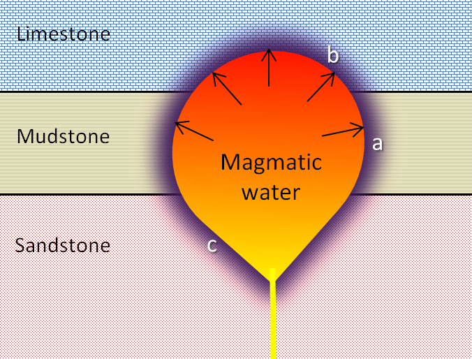
![Figure 8.1 Arizona’s Grand Canyon is an icon for geological time; 1,450 million years are represented by this photo. The light-coloured layered rocks at the top formed at around 250 Ma, and the dark ones at the bottom (within the steep canyon) at around 1,700 Ma. [SE]](http://opentextbc.ca/geology/wp-content/uploads/sites/110/2015/07/Arizona’s-Grand-Canyon.jpg)
![Figure 8.2 William Smith’s “Sketch of the succession of strata and their relative altitudes,” an inset on his geological map of England and Wales (with era names added). [SE after: http://earthobservatory.nasa.gov/Features/WilliamSmith/images/sketch_of_the_succession_of_strata.jpg]](http://opentextbc.ca/geology/wp-content/uploads/sites/110/2015/07/geological-map-of-England-and-Wales.png)
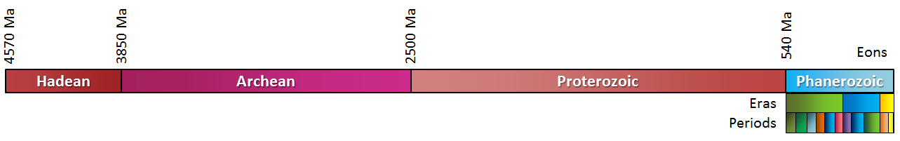
![Figure 8.4 The eras (middle row) and periods (bottom row) of the Phanerozoic [SE]](http://opentextbc.ca/geology/wp-content/uploads/sites/110/2015/07/Phanerozoic.png)
![Figure 8.5 The periods (middle row) and epochs (bottom row) of the Cenozoic [SE]](http://opentextbc.ca/geology/wp-content/uploads/sites/110/2015/07/Cenozoic.png)
![Figure 8.6a A xenolith of diorite incorporated into a basalt lava flow, Mauna Kea volcano, Hawaii. The lava flow took place some time after the diorite cooled, was uplifted, and then eroded. (Hammerhead for scale) [SE]](http://opentextbc.ca/geology/wp-content/uploads/sites/110/2015/07/xenolith-of-diorite.jpg)
![Figure 8.6b Rip-up clasts of shale embedded in Gabriola Formation sandstone, Gabriola Island, B.C. The pieces of shale were eroded as the sandstone was deposited, so the shale is older than the sandstone. [SE]](http://opentextbc.ca/geology/wp-content/uploads/sites/110/2015/07/sandstone.jpg)
![Figure 8.7 Superposition and cross-cutting relationships in Cretaceous Nanaimo Group rocks in Nanaimo, B.C. The coal seam is about 50 cm thick. [SE ]](https://opentextbc.ca/physicalgeologyearle/wp-content/uploads/sites/145/2016/03/cavan-2.png)
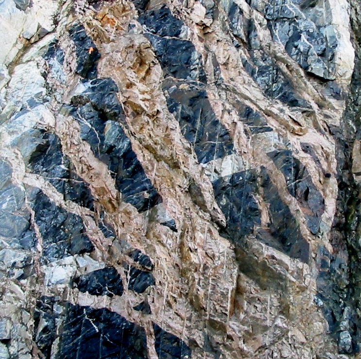
![Figure 8.8 The great angular unconformity in the Grand Canyon, Arizona. The tilted rocks at the bottom are part of the Proterozoic Grand Canyon Group (aged 825 to 1,250 Ma). The flat-lying rocks at the top are Paleozoic (540 to 250 Ma). The boundary between the two (which is marked, where visible, with a dashed white line) represents a time gap of nearly 300 million years. [SE ]](http://opentextbc.ca/geology/wp-content/uploads/sites/110/2015/07/Grand-Canyon.jpg)
![Figure 8.9 The four types of unconformities: a: a nonconformity between non-sedimentary rock and sedimentary rock, b: an angular unconformity , c: a disconformity between layers of sedimentary rock, where the older rock has been eroded but not tilted, and d: a paraconformity where there is a long period (millions of years) of non-deposition between two parallel layers. [SE ]](http://opentextbc.ca/geology/wp-content/uploads/sites/110/2015/07/unconformities.png)
![Figure 8.10 A summary of life on Earth during the late Proterozoic and the Phanerozoic. The top row shows geological eras, and the lower row shows the periods. [SE]](http://opentextbc.ca/geology/wp-content/uploads/sites/110/2015/07/Proterozoic-and-the-Phanerozoic.png)
![Figure 8.11 The application of bracketing to constrain the age of a rock based on several fossils. In this diagram, the coloured bar represents the time range during which each of the four species (A – D) existed on Earth. Although each species lived for several million years, we can narrow down the likely age of the rock to just 0.7 Ma during which all four species co-existed. [SE]](http://opentextbc.ca/geology/wp-content/uploads/sites/110/2015/07/age-of-a-rock.png)
![Figure 8.12 The septum of an ammonite (white part, left), and the suture lines where the septae meet the outer shell (right). [SE]](http://opentextbc.ca/geology/wp-content/uploads/sites/110/2015/07/septum-of-an-ammonite.png)
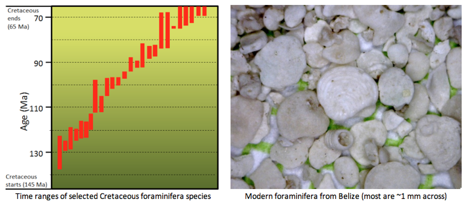
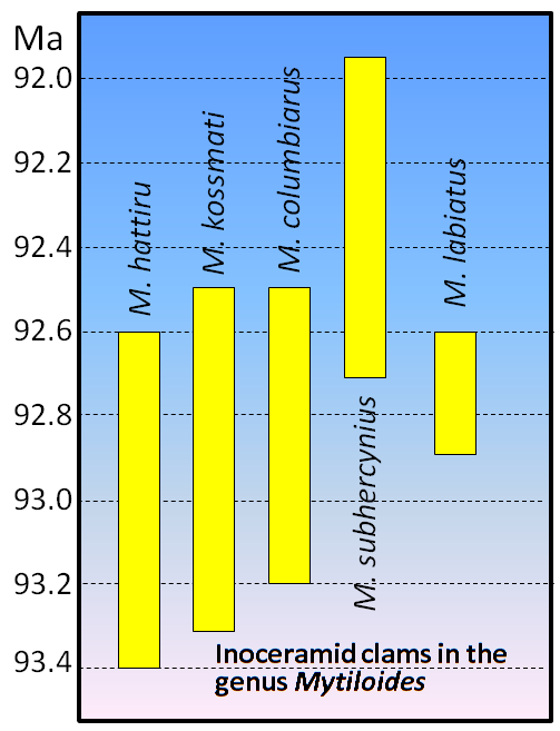
![Figure 8.14 The decay of 40K over time. Each half-life is 1.3 billion years, so after 3.9 billion years (three half-lives) 12.5% of the original 40K will remain. The red-blue bars represent 40K and the green-yellow bars represent 40Ar. [SE]](https://opentextbc.ca/physicalgeologyearle/wp-content/uploads/sites/145/2016/03/decay-of-40K.png)
![Figure 8.15 Crystals of potassium feldspar (pink) in a granitic rock are candidates for isotopic dating using the K-Ar method because they contained potassium and no argon when they formed. [SE]](http://opentextbc.ca/geology/wp-content/uploads/sites/110/2015/07/Crystals-of-potassium-feldspar.jpg)
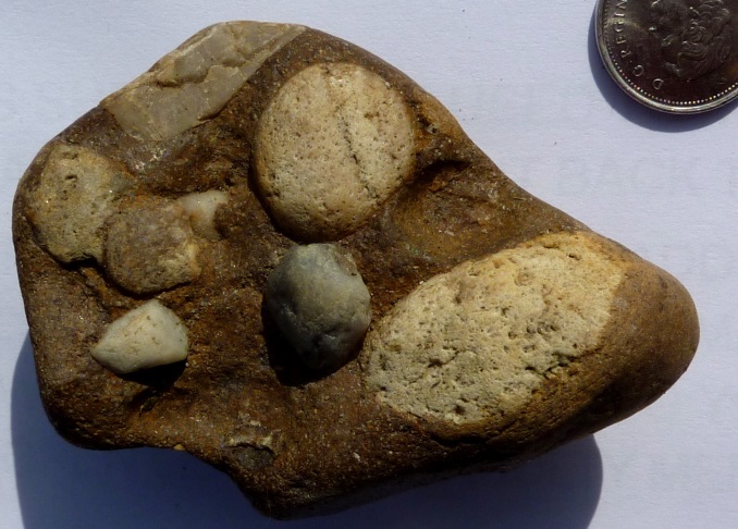
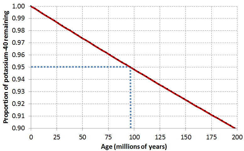 An example is provided (in blue) for a 40K proportion of 0.95, which is equivalent to an age of approximately 96 Ma. This is determined by drawing a horizontal line from 0.95 to the decay curve line, and then a vertical line from there to the time axis. [SE]
![Figure 8.16 Radiocarbon dates on wood fragments in glacial sediments in the Strait of Georgia [SE after Clague, J, 1976, Quadra Sand and its relation to late Wisconsin glaciation of southeast British Columbia, Can. J. Earth Sciences, V. 13, p. 803-815]](http://opentextbc.ca/geology/wp-content/uploads/sites/110/2015/07/Radiocarbon.png)
![Figure 8.17 Example of tree-ring dating of dead trees [SE]](http://opentextbc.ca/geology/wp-content/uploads/sites/110/2015/07/tree-ring-dating.png)
![Figure 8.18 Sites in Washington where dead trees are present in coastal flats. The outermost wood of eight trees was dated using dendrochronology, and of these, seven died during the year 1699, suggesting that the land was inundated by water at that time. [SE from data in Yamaguchi, D.K., B.F. Atwater, D.E. Bunker, B.E. Benson, and M.S. Reid. 1997. Tree-ring dating the 1700 Cascadia earthquake. Nature, Vol. 389, pp. 922 - 923, 30 October 1997.]](http://opentextbc.ca/geology/wp-content/uploads/sites/110/2015/07/Washington.png)
![Figure 8.19 The last 5 Ma of magnetic field reversals. [SE after U.S. Geological Survey, http://upload.wikimedia.org/wikipedia/commons/1/13/Geomagnetic_polarity_late_Cenozoic.svg.]](http://opentextbc.ca/geology/wp-content/uploads/sites/110/2015/07/magnetic-field-reversals.png)
![Figure 8.20 Depiction of the formation of magnetized oceanic crust at a spreading ridge. Coloured bars represent periods of normal magnetism, and the small capital letters denote the Brunhes, Jaramillio, Olduvai, and Gauss normal magnetic periods (see Figure 8.15). [SE]](http://opentextbc.ca/geology/wp-content/uploads/sites/110/2015/07/magnetized-oceanic-crust.png)
![Figure 8.21 The pattern of magnetism within the area of the Juan de Fuca Plate, off the west coast of North America. The coloured shapes represent parts of the sea floor that have normal magnetism, and the magnetic time scale is shown using the same colours. The blue bands represent Brunhes, Jaramillo, and Olduvai, the green represents Gauss, and so on. (Note that, in this diagram, sea-floor magnetism is only shown for the Juan de Fuca Plate, although similar patterns exist on the Pacific Plate.) [SE]](http://opentextbc.ca/geology/wp-content/uploads/sites/110/2015/07/pattern-of-magnetism.png)
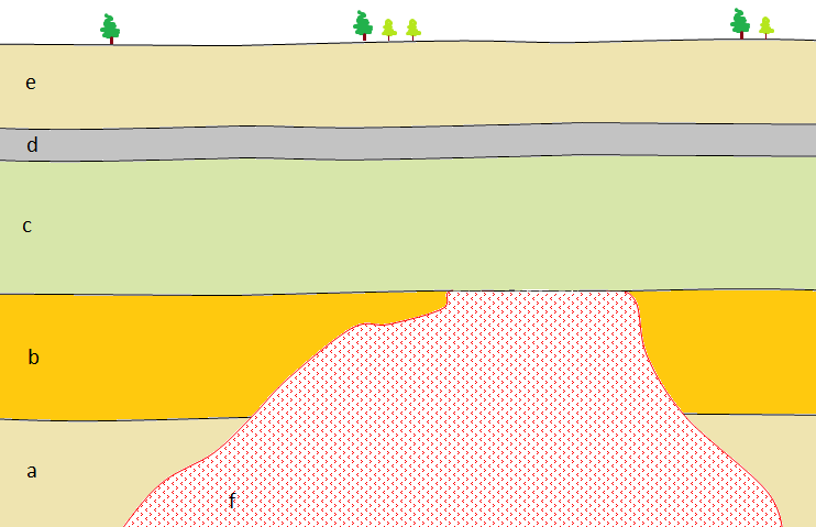
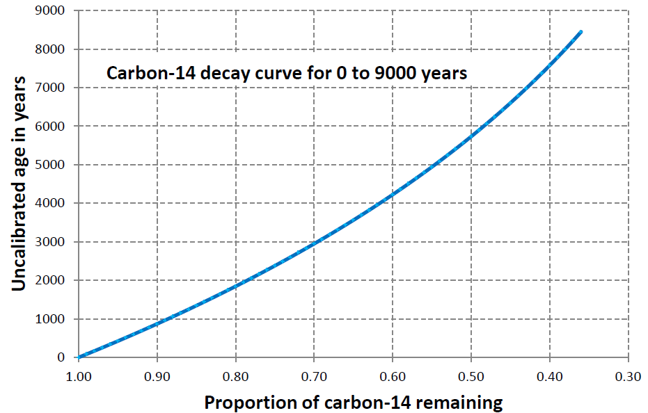
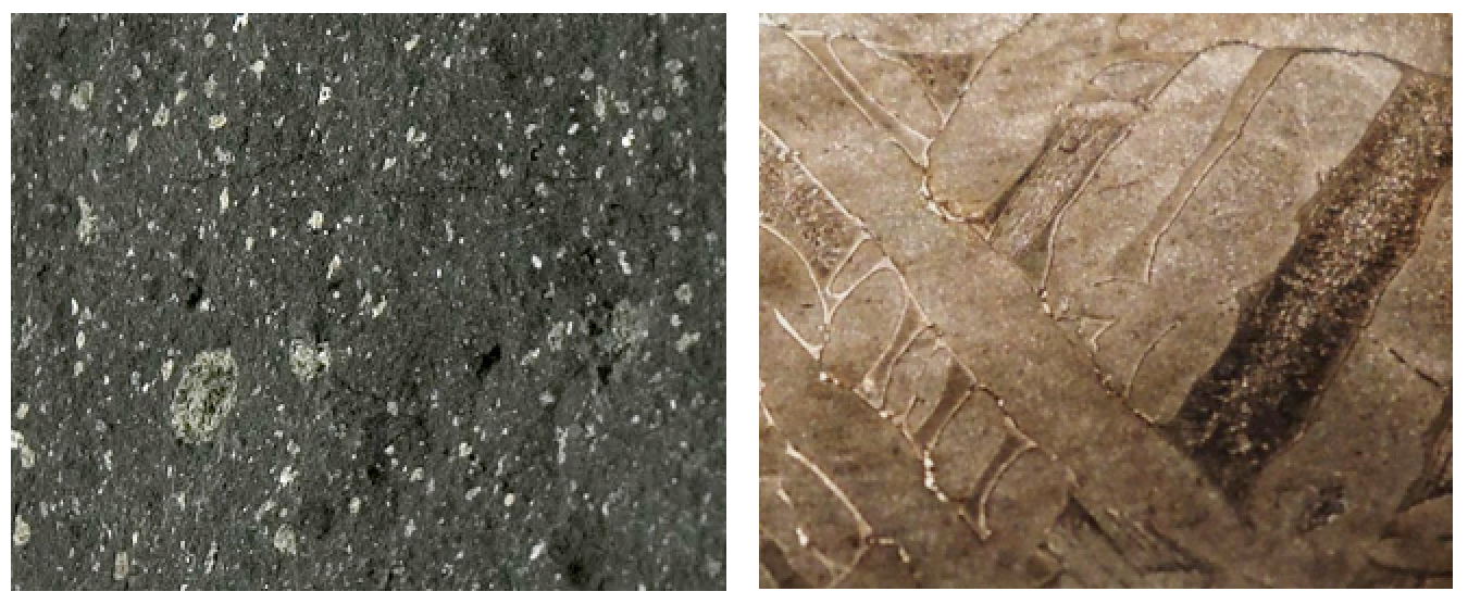
![Figure 9.2 Earth’s layers: crust is pink, mantle is green, core is blue [SE]](https://opentextbc.ca/physicalgeologyearle/wp-content/uploads/sites/145/2016/06/9-earth-interior.png)
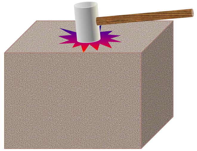
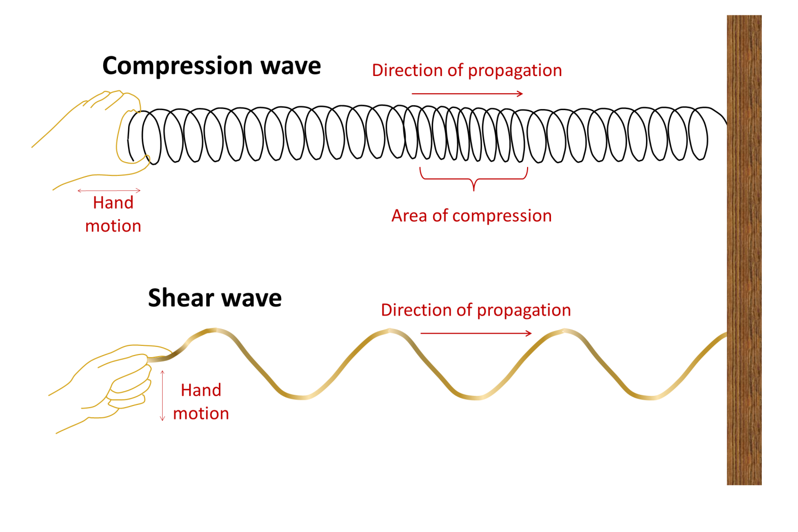

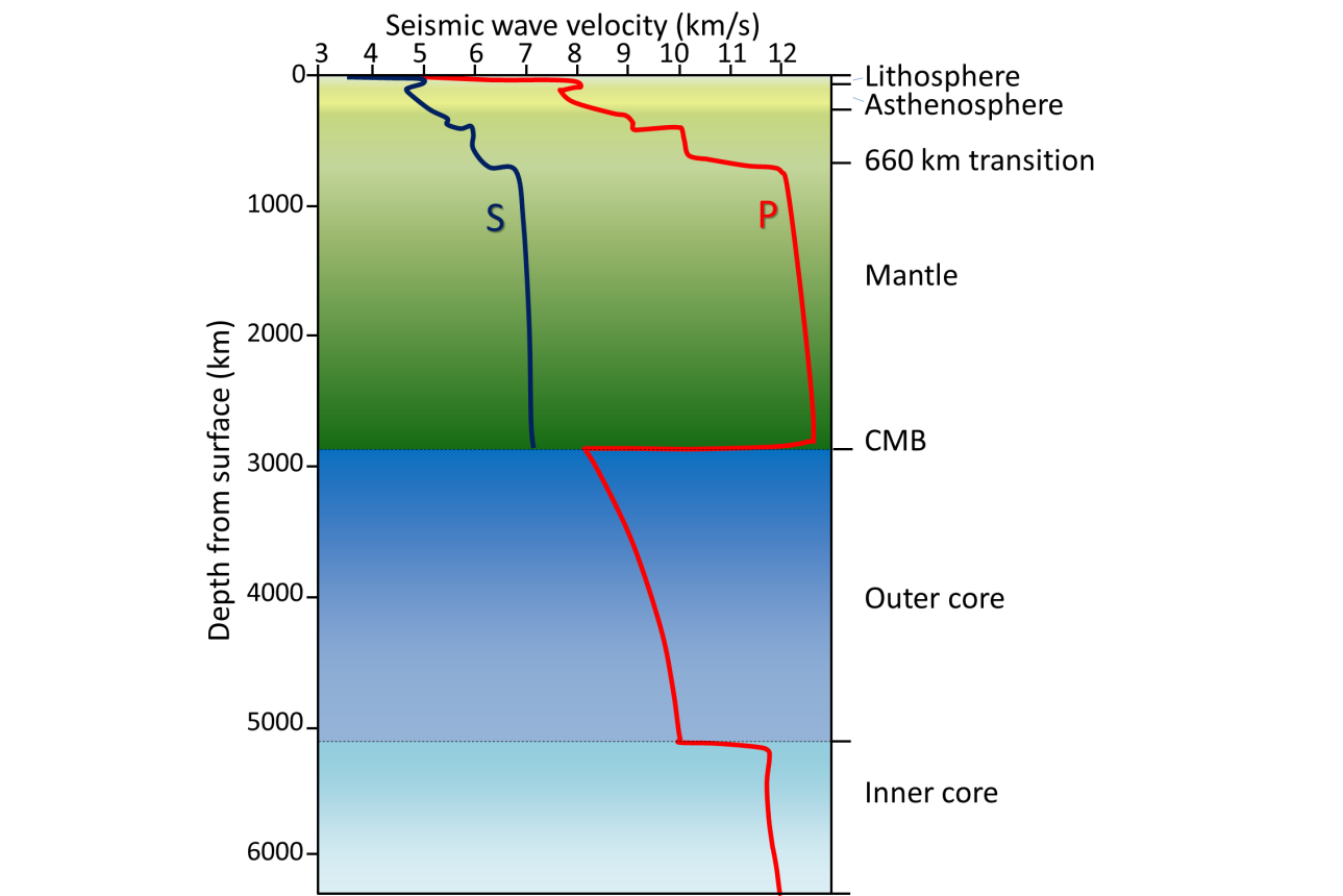
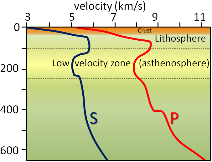
![Figure 9.7 Depiction of seismic waves emanating from an earthquake (red star). Some waves travel through the crust to the seismic station (at about 6 km/s), while others go down into the mantle (where they travel at around 8 km/s) and are bent upward toward the surface, reaching the station before the ones that travelled only through the crust. [SE]](https://opentextbc.ca/physicalgeologyearle/wp-content/uploads/sites/145/2016/06/moho.png)
![Figure 9.8 Patterns of seismic wave propagation through Earth’s mantle and core. S-waves do not travel through the liquid outer core, so they leave a shadow on Earth’s far side. P-waves do travel through the core, but because the waves that enter the core are refracted, there are also P-wave shadow zones. [SE]](https://opentextbc.ca/physicalgeologyearle/wp-content/uploads/sites/145/2016/06/shadow-2.png)
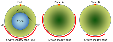
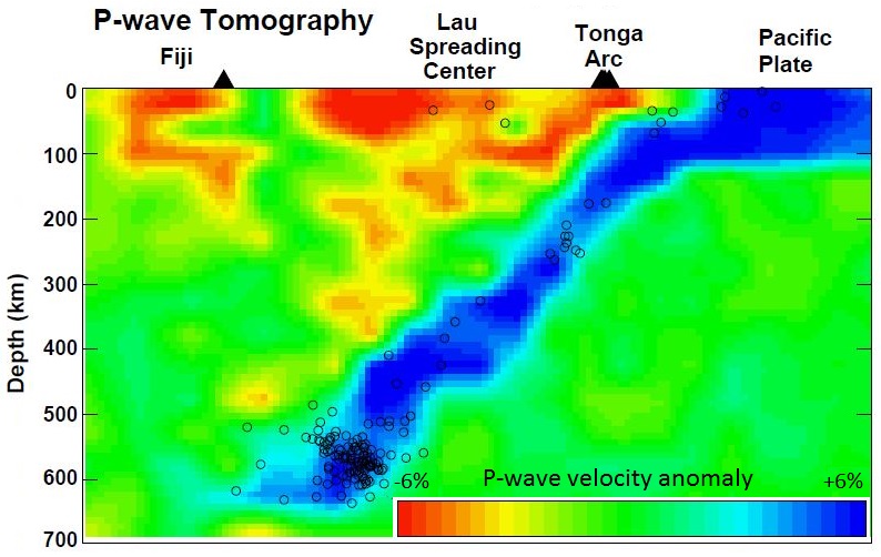
![Figure 9.10 Generalized rate of temperature increase with depth within Earth. Temperature increases to the right, so the flatter the line, the steeper the temperature gradient. Our understanding of the temperature gradient comes from seismic wave information and knowledge of the melting points of Earth’s materials. [SE]](https://opentextbc.ca/physicalgeologyearle/wp-content/uploads/sites/145/2016/06/temp-profile-1.png)
![Figure 9.11 Rate of temperature increase with depth in Earth’s upper 500 km, compared with the dry mantle rock melting curve (red dashed line). LVZ= low-velocity zone [SE]](https://opentextbc.ca/physicalgeologyearle/wp-content/uploads/sites/145/2016/03/temp-profile-2.png)

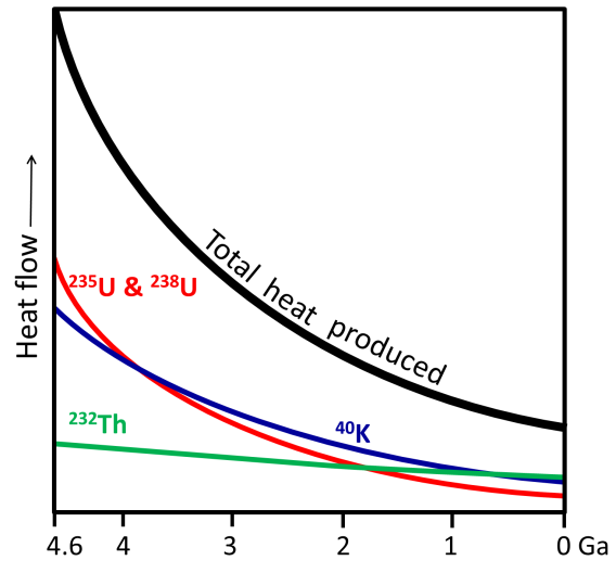
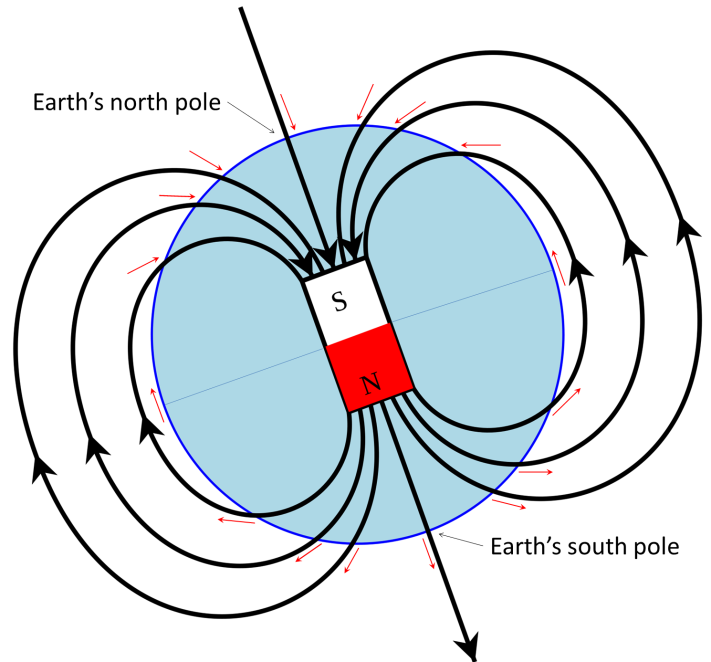
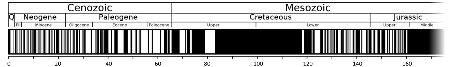
![Figure 9.15 Depiction of Earth’s magnetic field between reversals (left) and during a reversal (right). The lines represent magnetic field lines: blue where the field points toward Earth’s centre and yellow where it points away. The rotation axis of Earth is vertical, and the outline of the core is shown as a dashed white circle. [from: http://en.wikipedia.org/wiki/Geomagnetic_reversal]](https://opentextbc.ca/physicalgeologyearle/wp-content/uploads/sites/145/2016/06/glatzmeir-2.png)
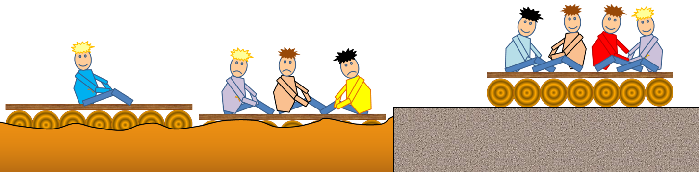
![Figure 9.17 Illustration of the isostatic relationship between the crust and the mantle. Following a period of mountain building, mass has been added to a part of the crust, and the thickened crust has pushed down into the mantle (left). Over the following tens of millions of years, the mountain chain is eroded and the crust rebounds (right). The green arrows represent slow mantle flow. [SE]](https://opentextbc.ca/physicalgeologyearle/wp-content/uploads/sites/145/2016/06/rebound-2.png)
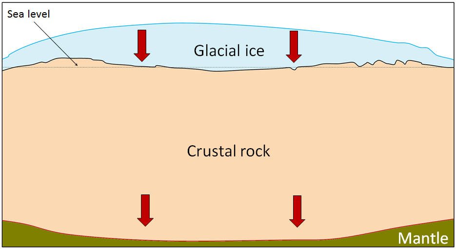
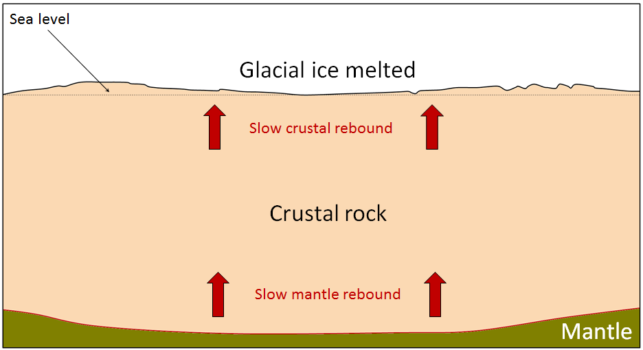
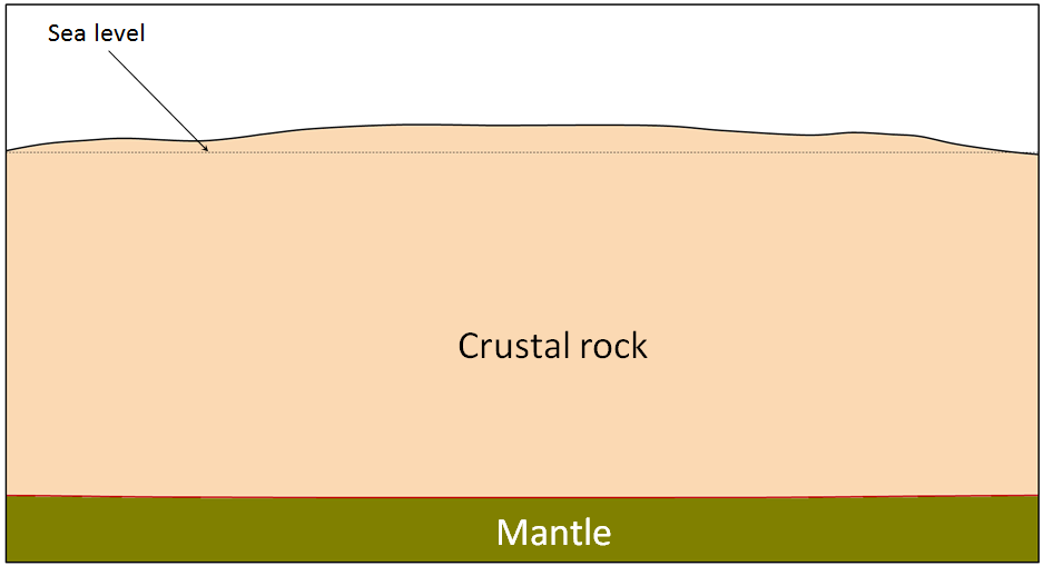
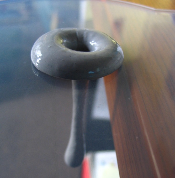

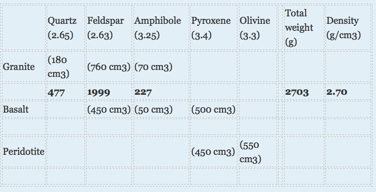

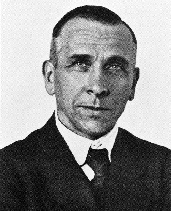
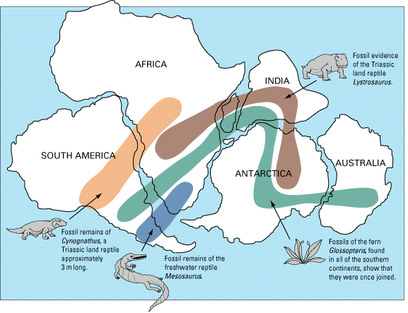

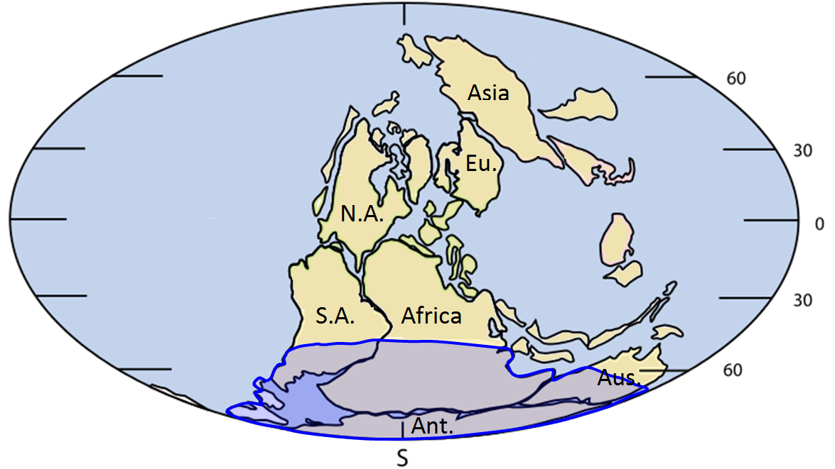
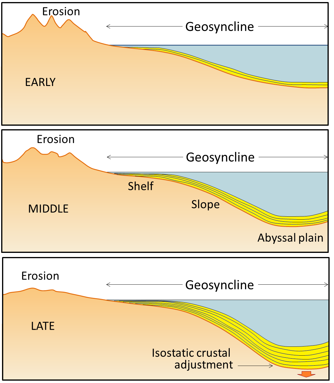
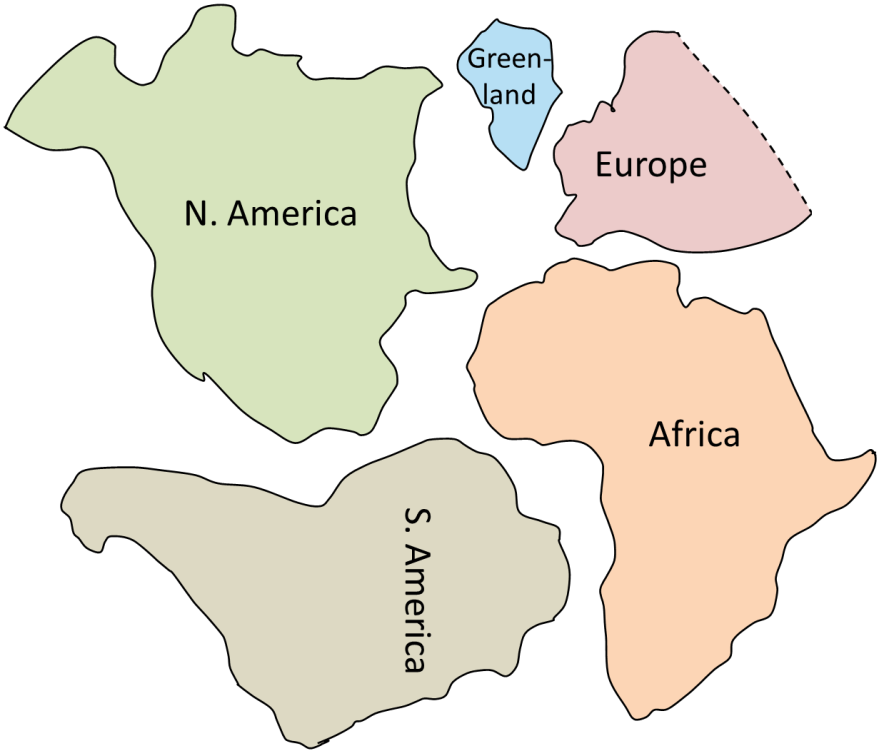
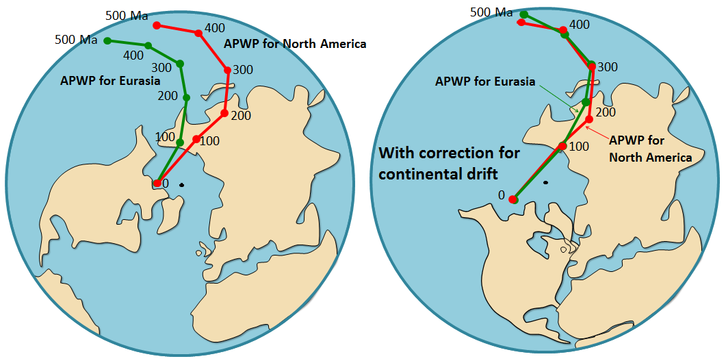
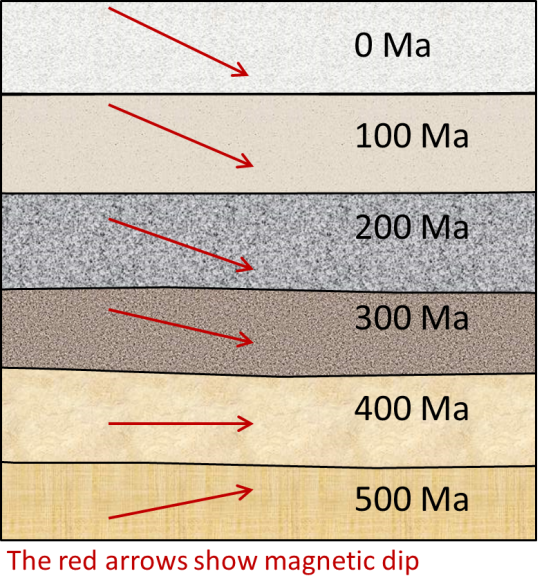
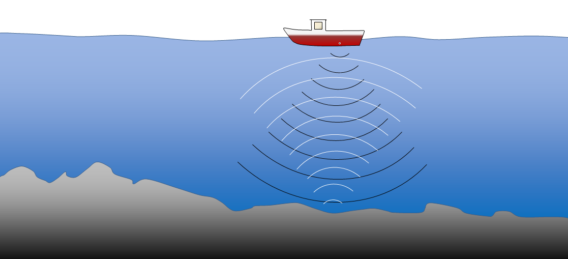
![Figure 10.8 Ocean floor bathymetry (and continental topography). Inset (a): the mid-Atlantic ridge, (b): the Newfoundland continental shelf, (c): the Nazca trench adjacent to South America, and (d): the Hawaiian Island chain. [SE after NOAA, http://upload.wikimedia.org/wikipedia/commons/9/93/Elevation.jpg]](https://opentextbc.ca/physicalgeologyearle/wp-content/uploads/sites/145/2016/03/bathymetry-2.png)
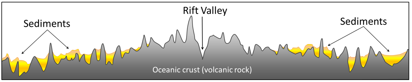

![Figure 10.11 Pattern of sea-floor magnetism off of the west coast of British Columbia and Washington [SE after http://geomaps.wr.usgs.gov/parks/noca/nocageol4c.html, adapted from: Raff, A and Mason, R, 1961, Magnetic survey off the west coast of North America, 40˚ N to 52˚ N latitude, Geol. Soc. America Bulletin, V. 72, p. 267-270.]](https://opentextbc.ca/physicalgeologyearle/wp-content/uploads/sites/145/2016/03/raff-mason.gif)
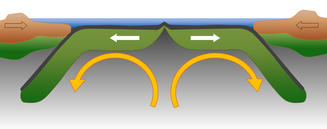
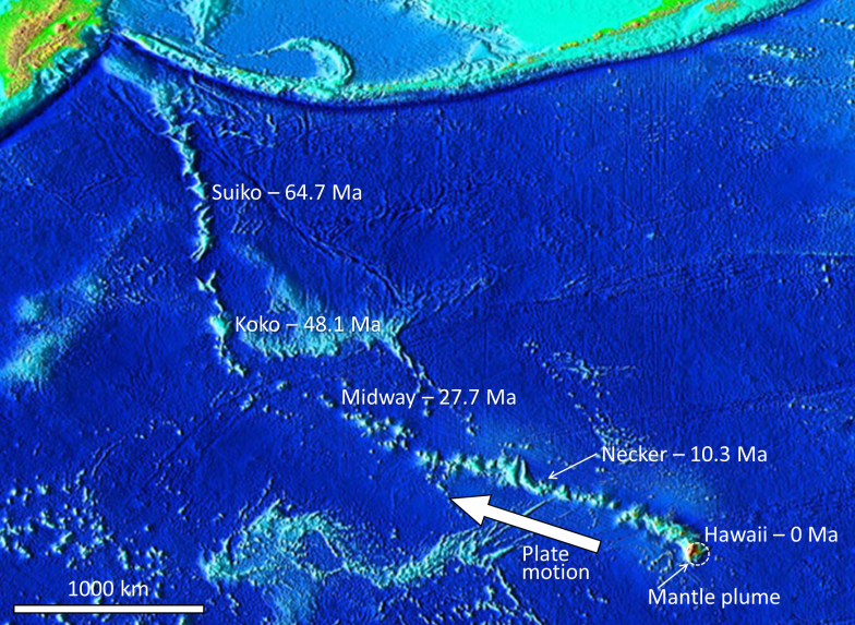
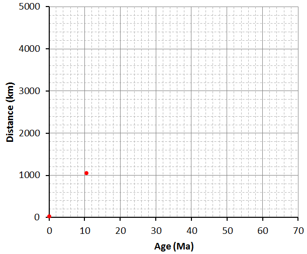
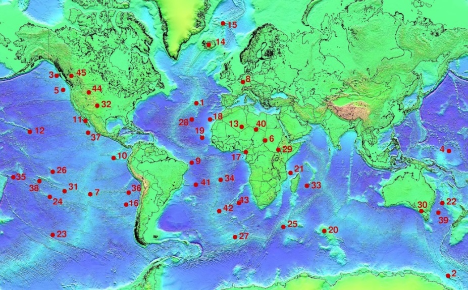
![Figure 10.15 A part of the mid-Atlantic ridge near the equator. The double white lines are spreading ridges. The solid white lines are fracture zones. As shown by the yellow arrows, the relative motion of the plates on either side of the fracture zones can be similar (arrows pointing the same direction) or opposite (arrows pointing opposite directions). Transform faults (red lines) are in between the ridge segments, where the yellow arrows point in opposite directions. [SE]](https://opentextbc.ca/physicalgeologyearle/wp-content/uploads/sites/145/2016/03/tranforms-2.png)
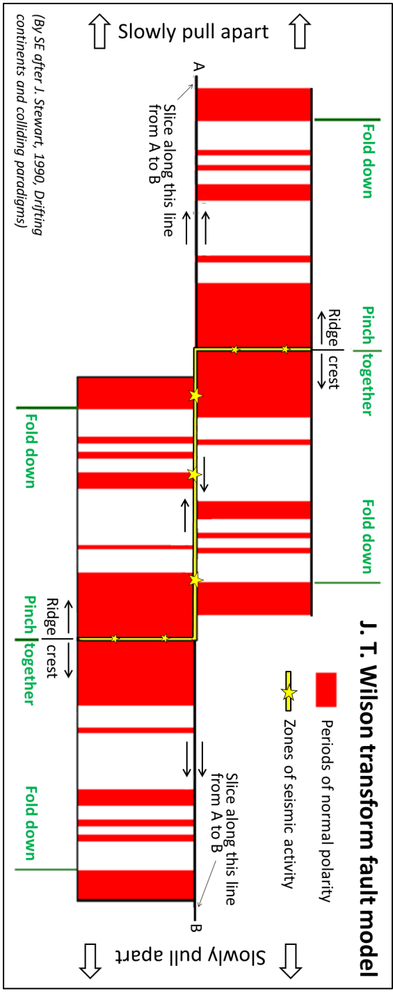
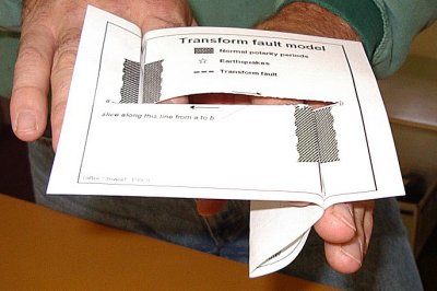
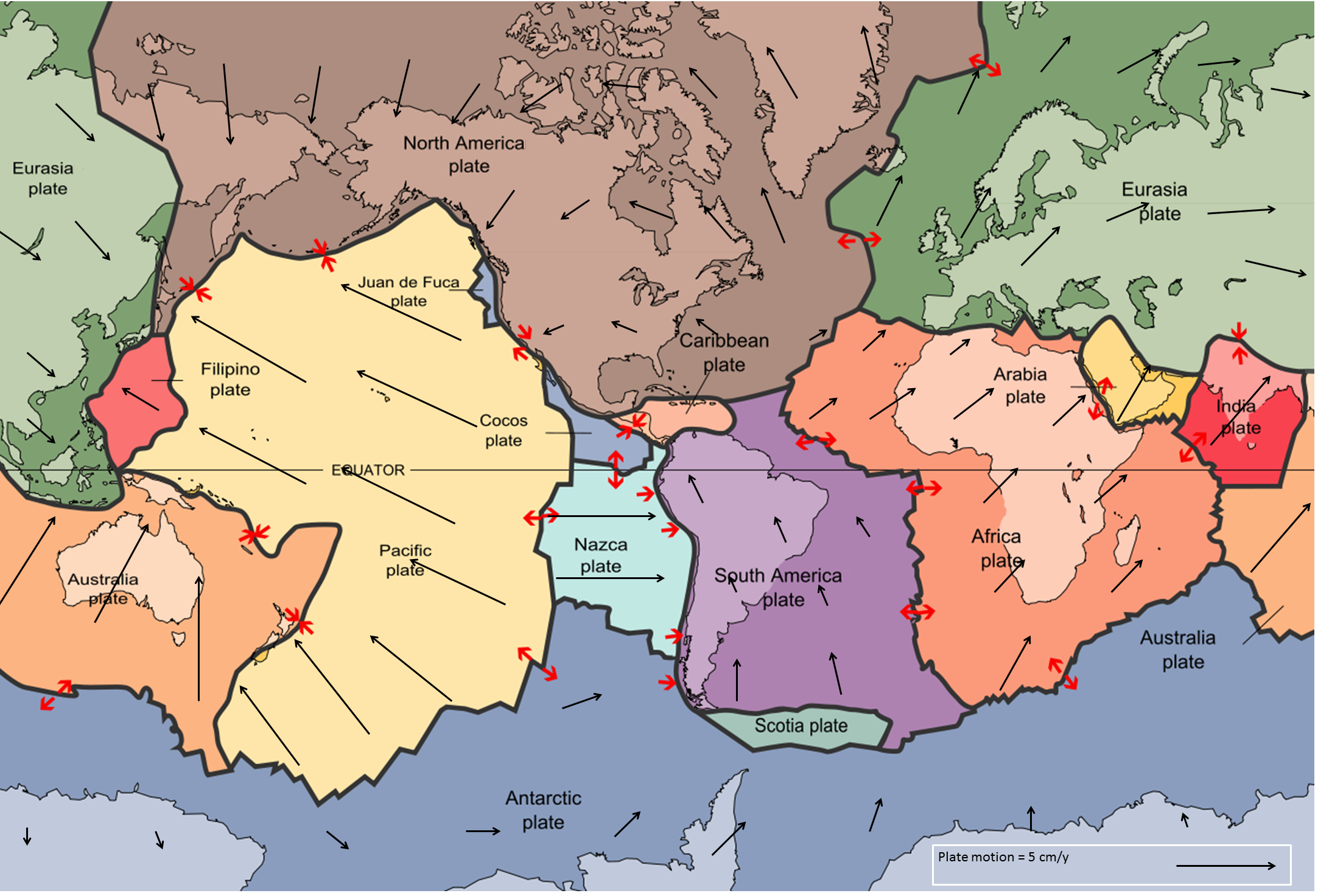

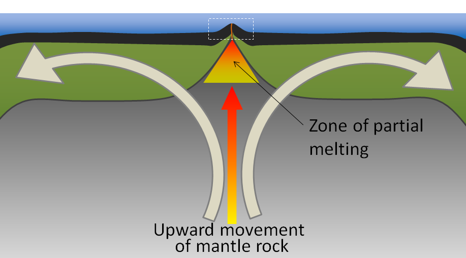
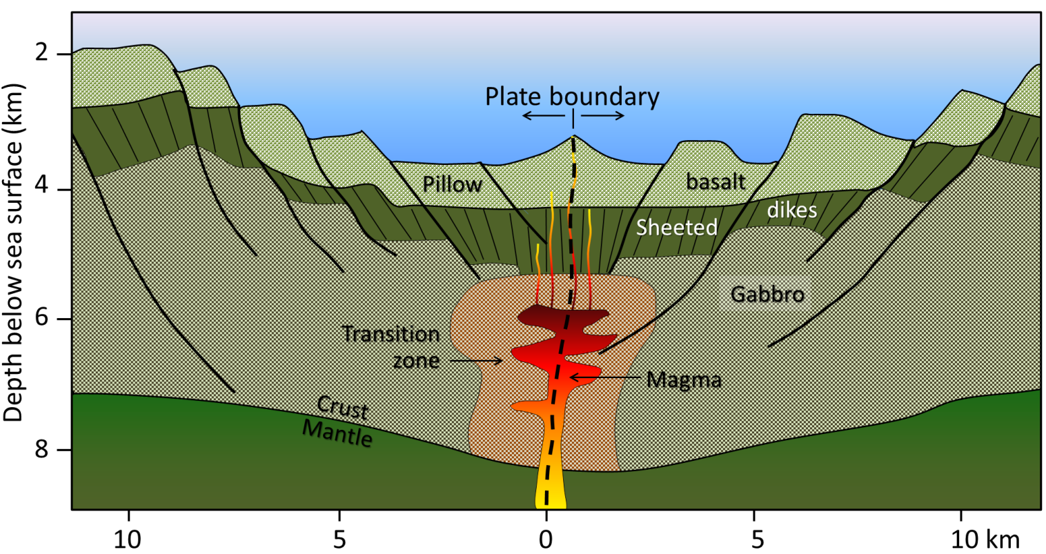
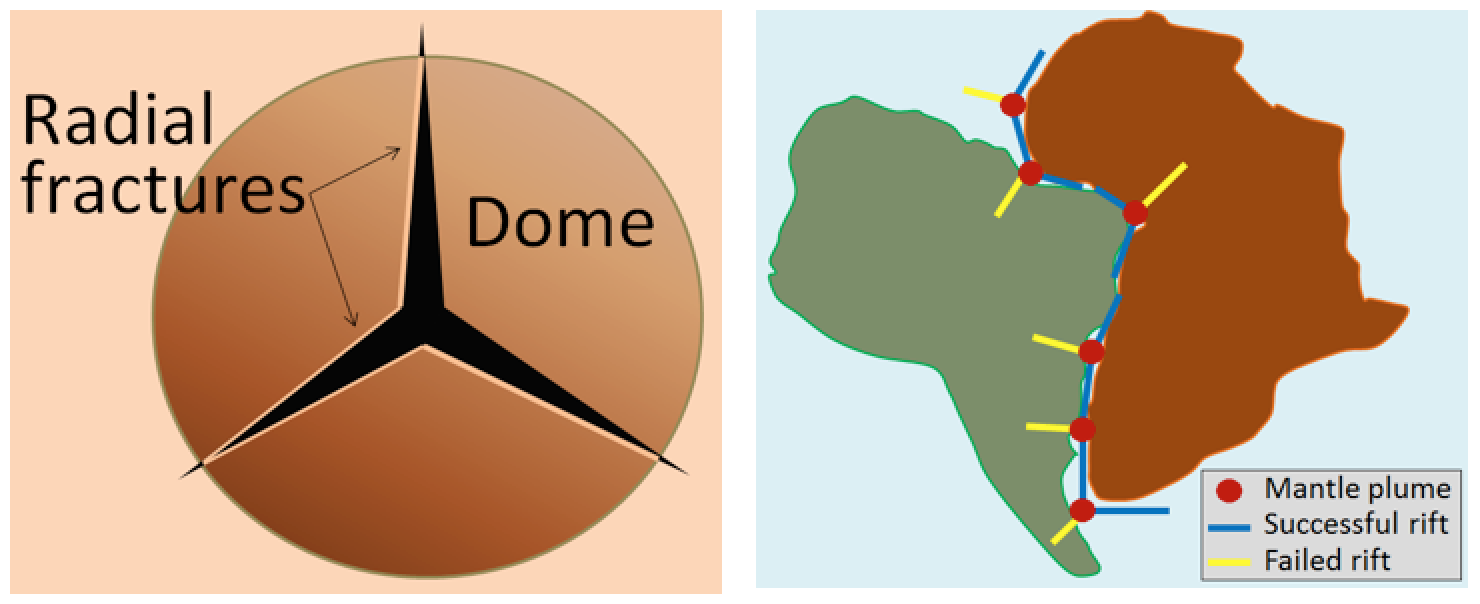
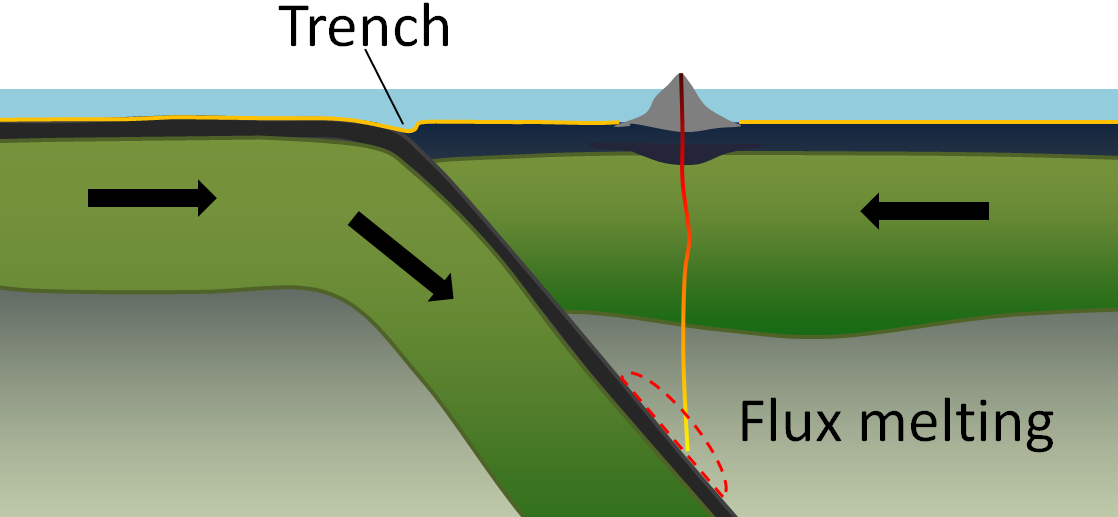
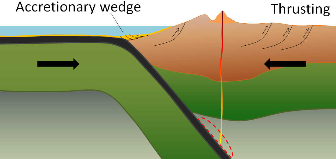
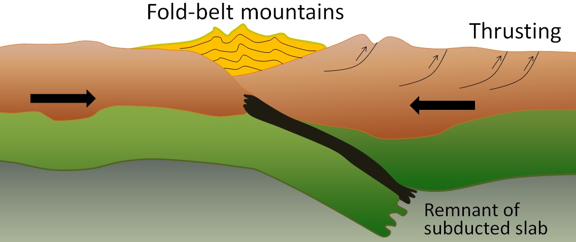
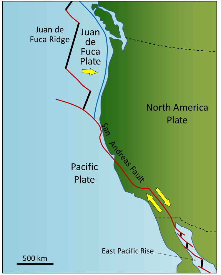
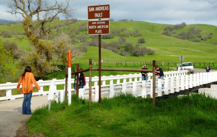
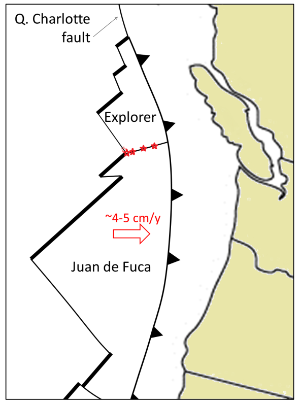
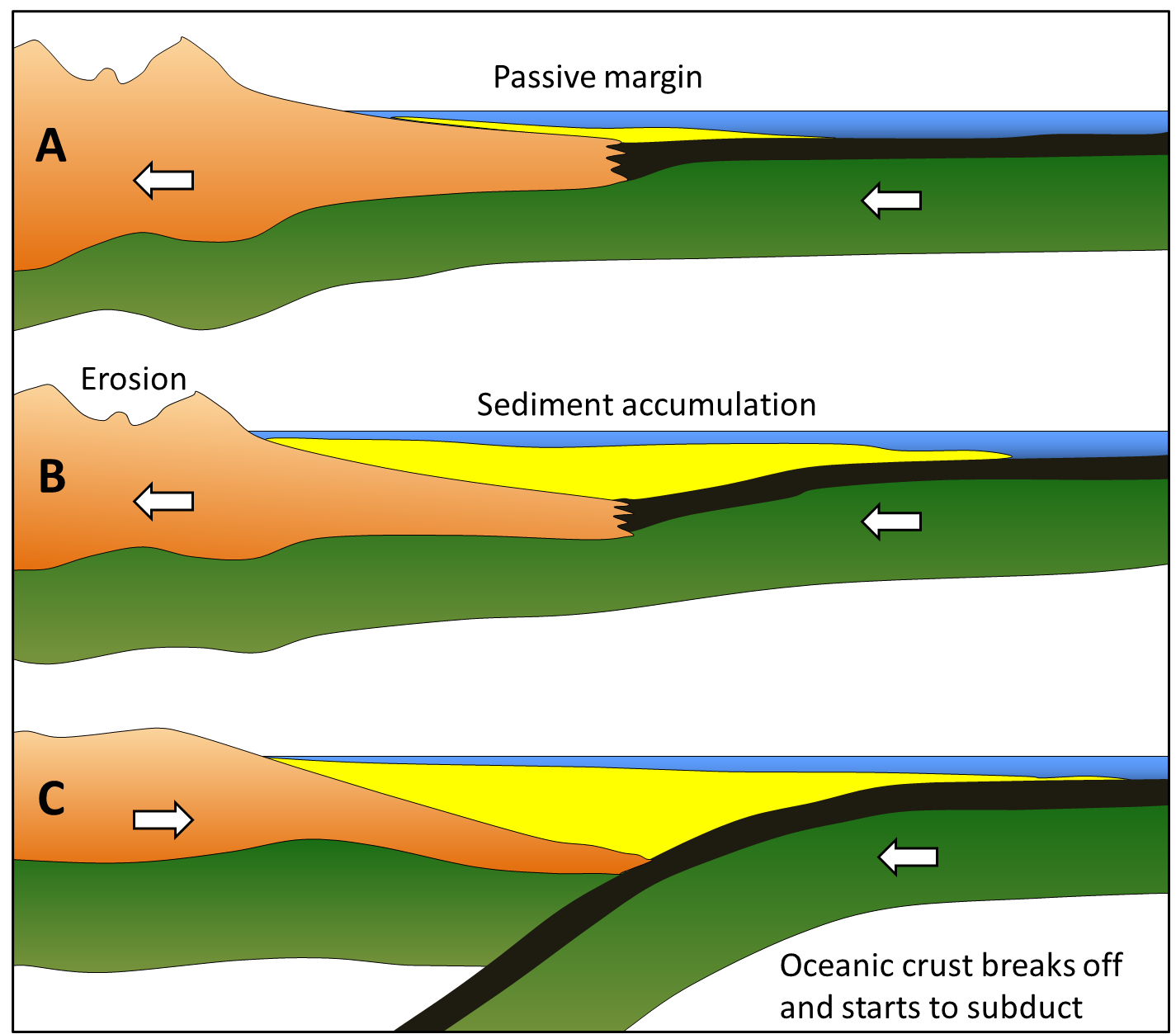
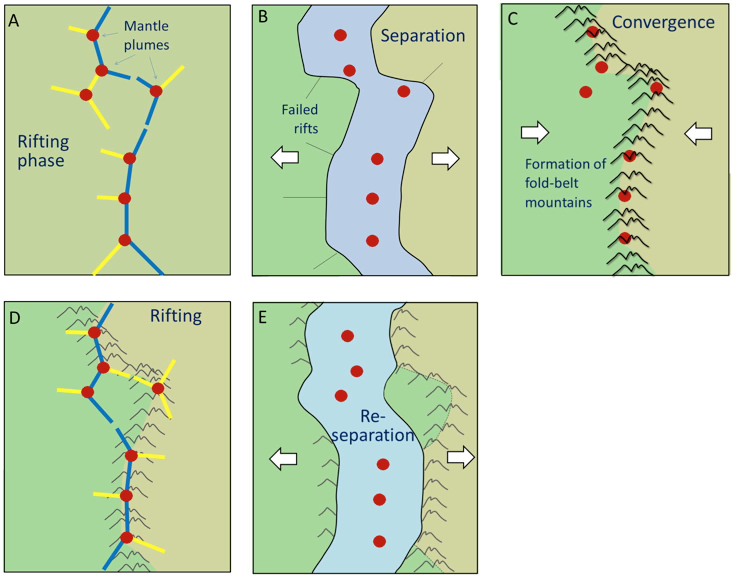

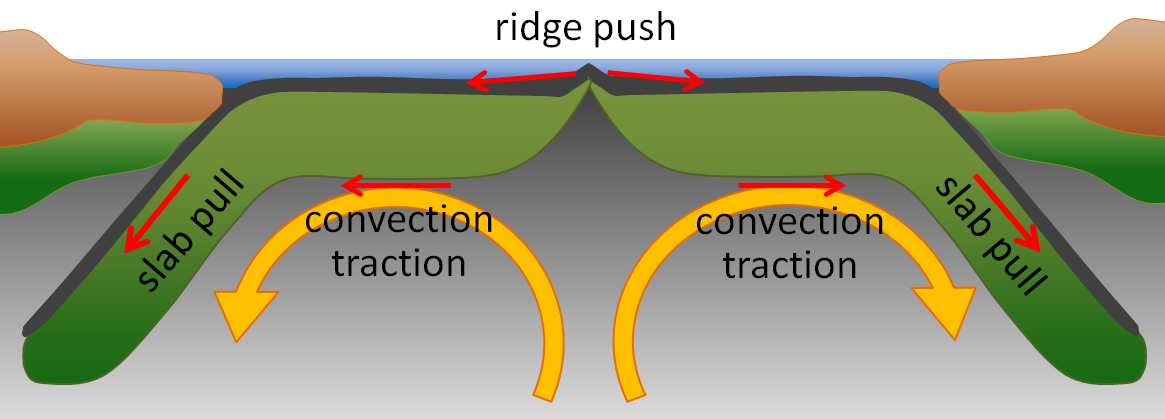
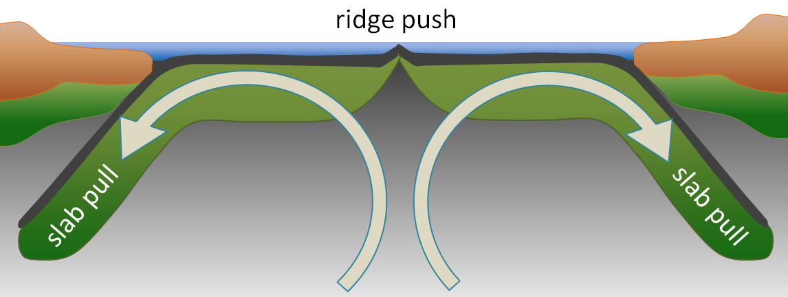


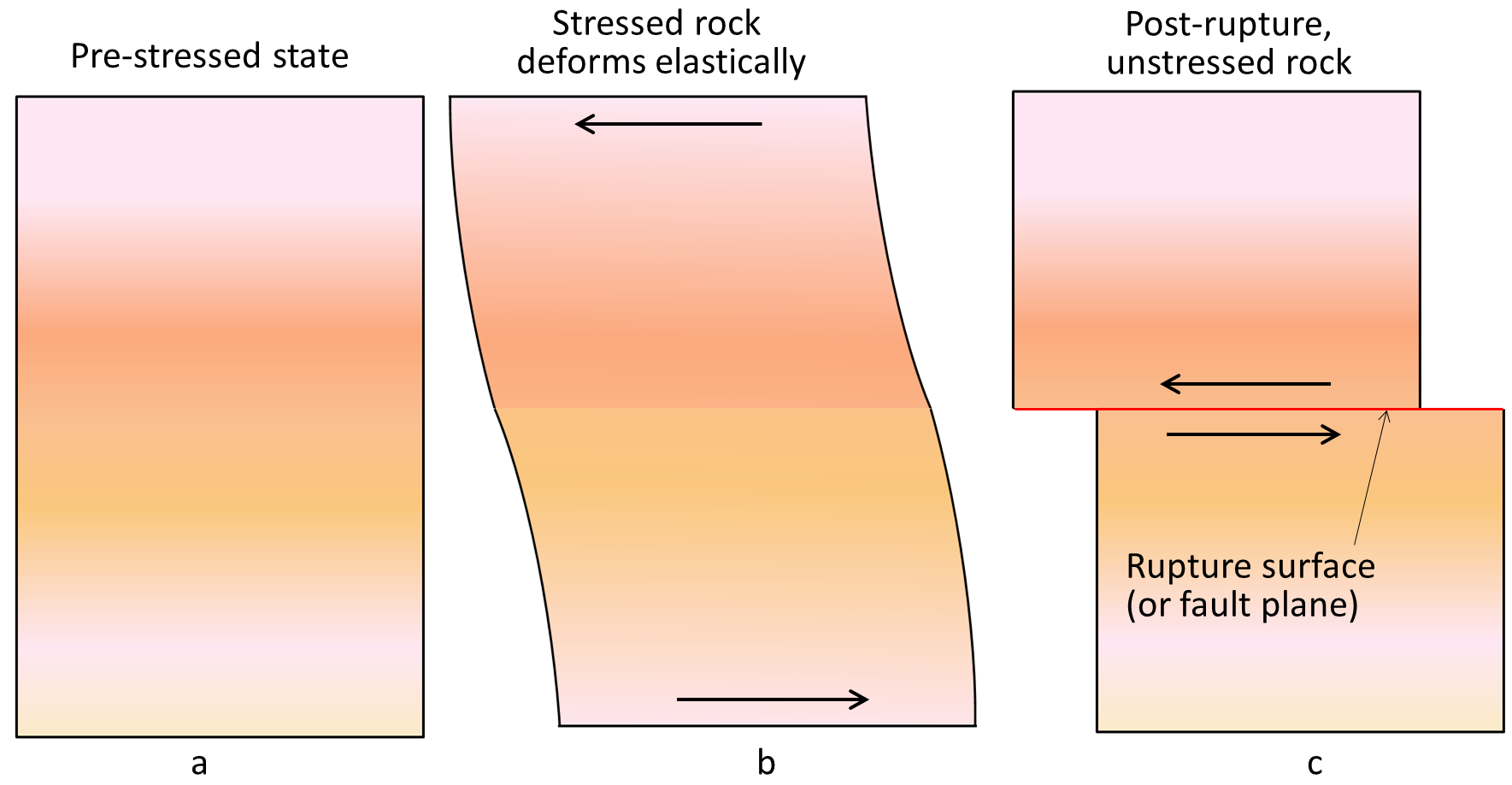
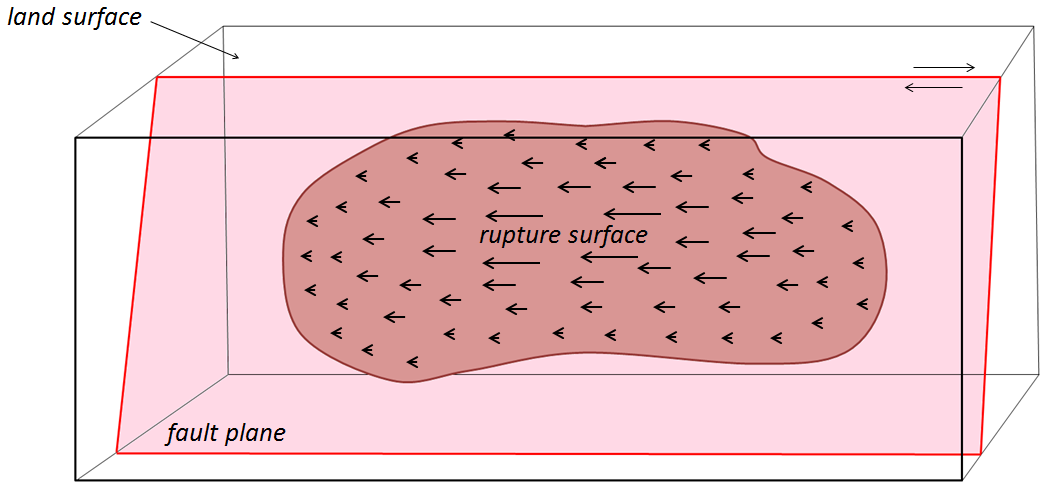
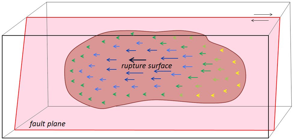

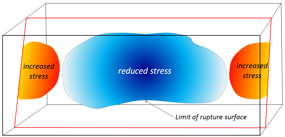
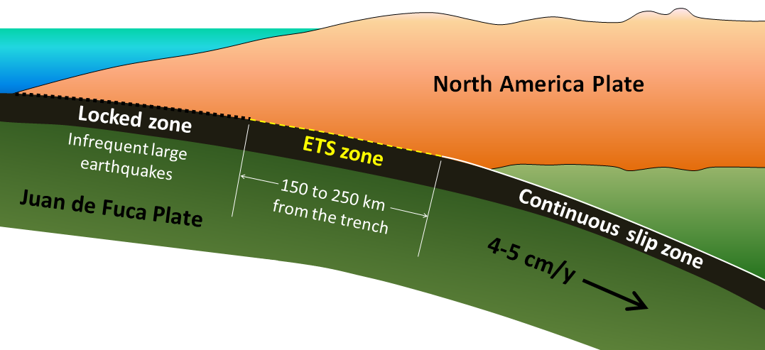
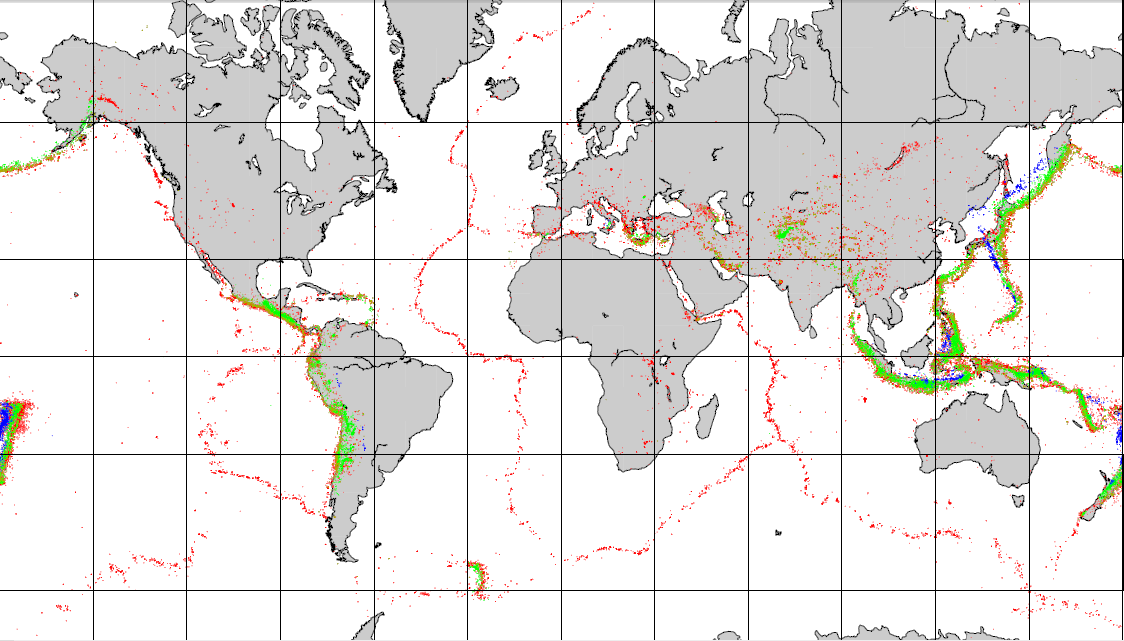
![Figure 11.8 Distribution of earthquakes of M4 and greater in the area of the mid-Atlantic ridge near the equator from 1990 to 1996. All are at a depth of 0 to 33 km [SE after Dale Sawyer, Rice University, http://plateboundary.rice.edu]](https://opentextbc.ca/physicalgeologyearle/wp-content/uploads/sites/145/2016/06/transform-quakes-2.png)
![Figure 11.9 Distribution of earthquakes of M4 and greater in the Central America region from 1990 to 1996 (red: 0-33 km, orange: 33-70 km, green: 70-300 km, blue: 300-700 km) (Spreading ridges are heavy lines, subduction zones are toothed lines, and transform faults are light lines.) [SE after Dale Sawyer, Rice University, http://plateboundary.rice.edu]](https://opentextbc.ca/physicalgeologyearle/wp-content/uploads/sites/145/2016/06/caribbean-2.png)
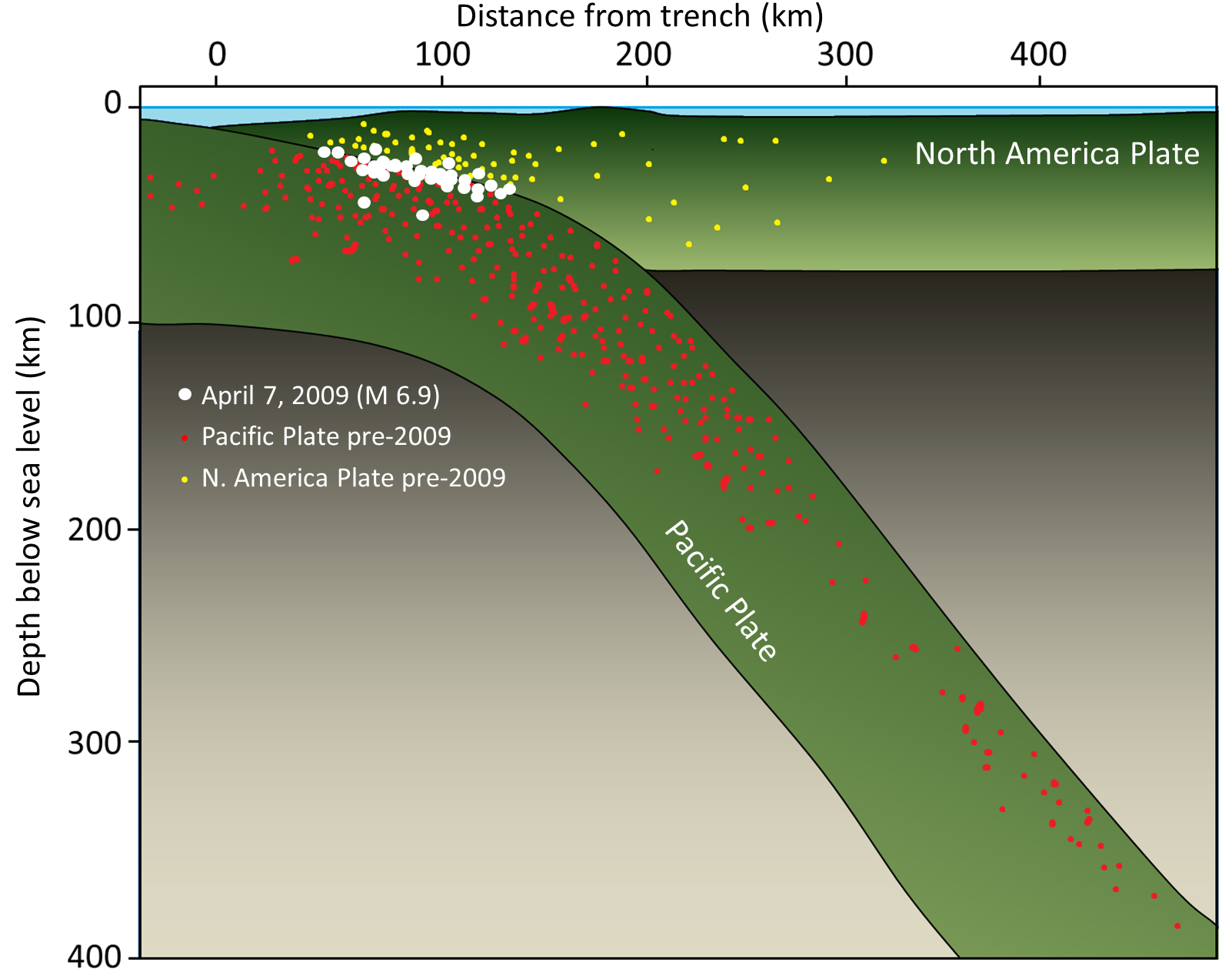
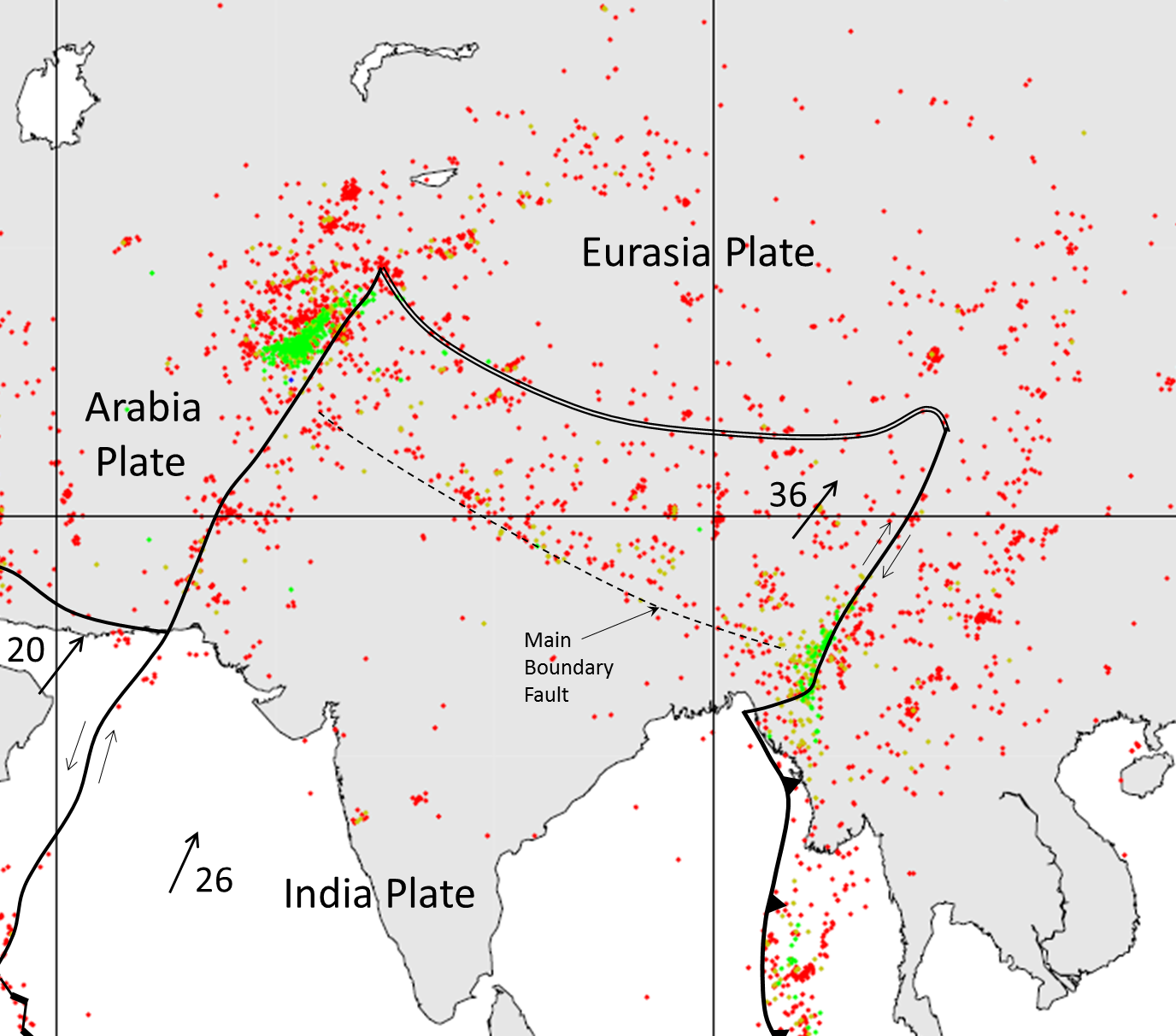

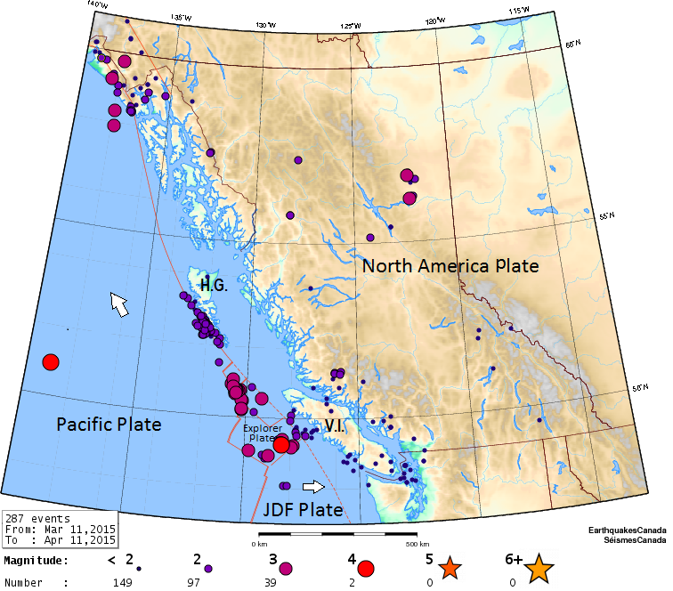
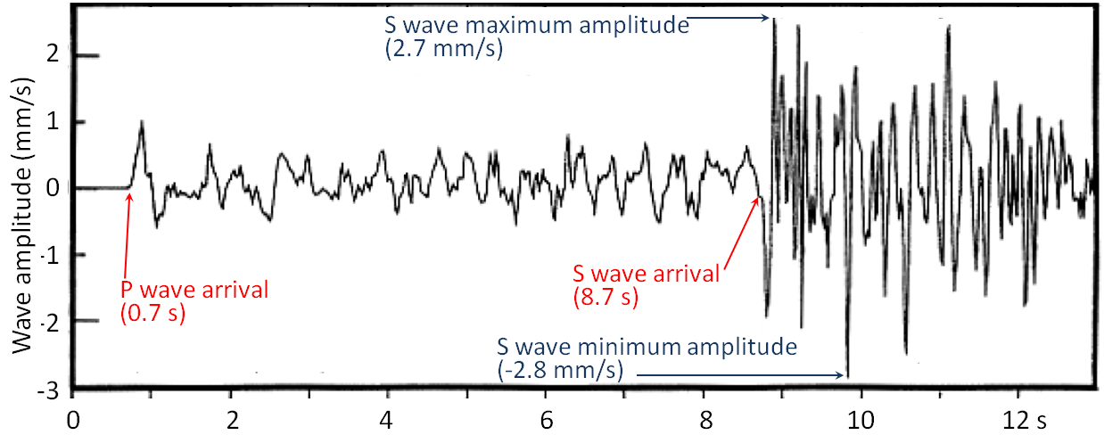
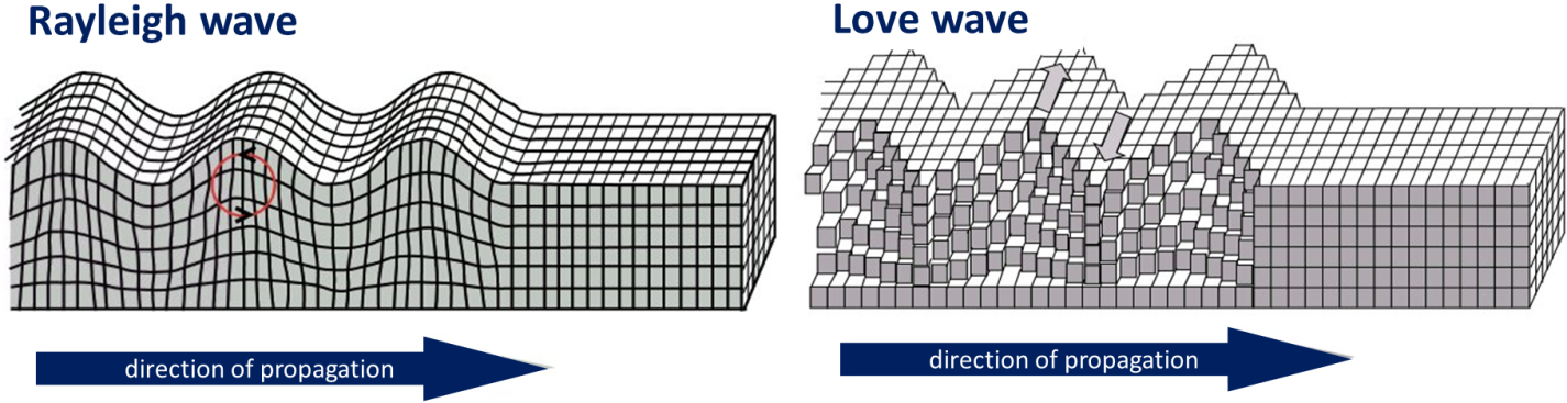
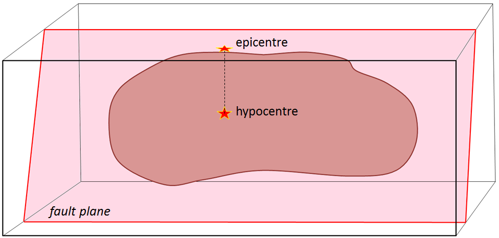
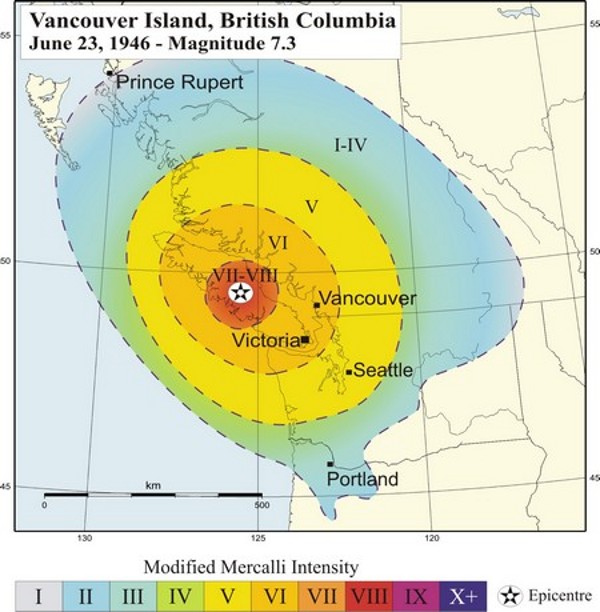
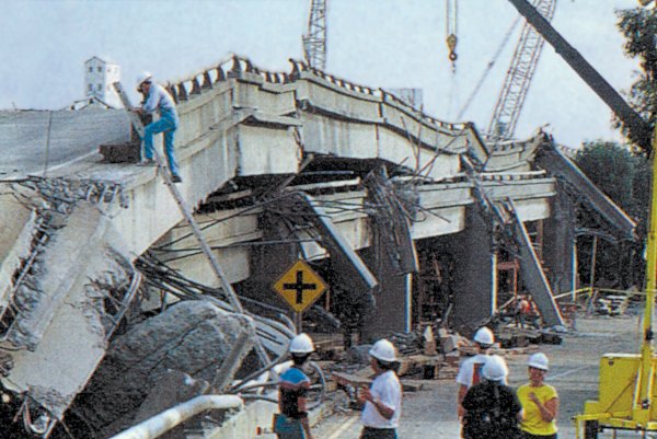
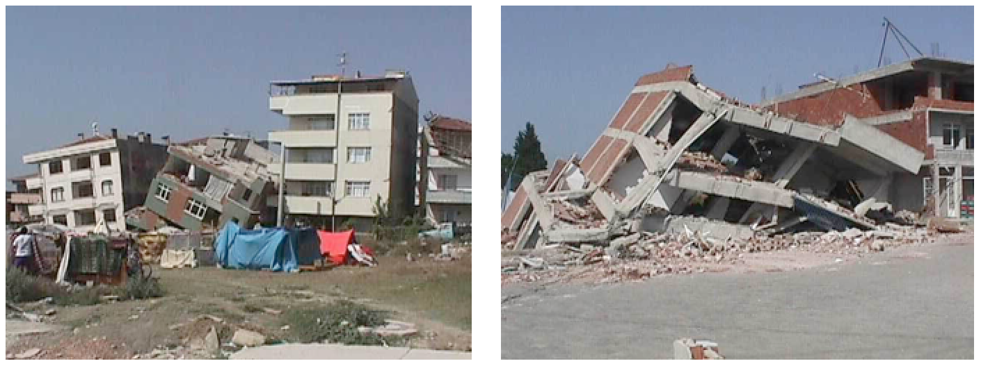
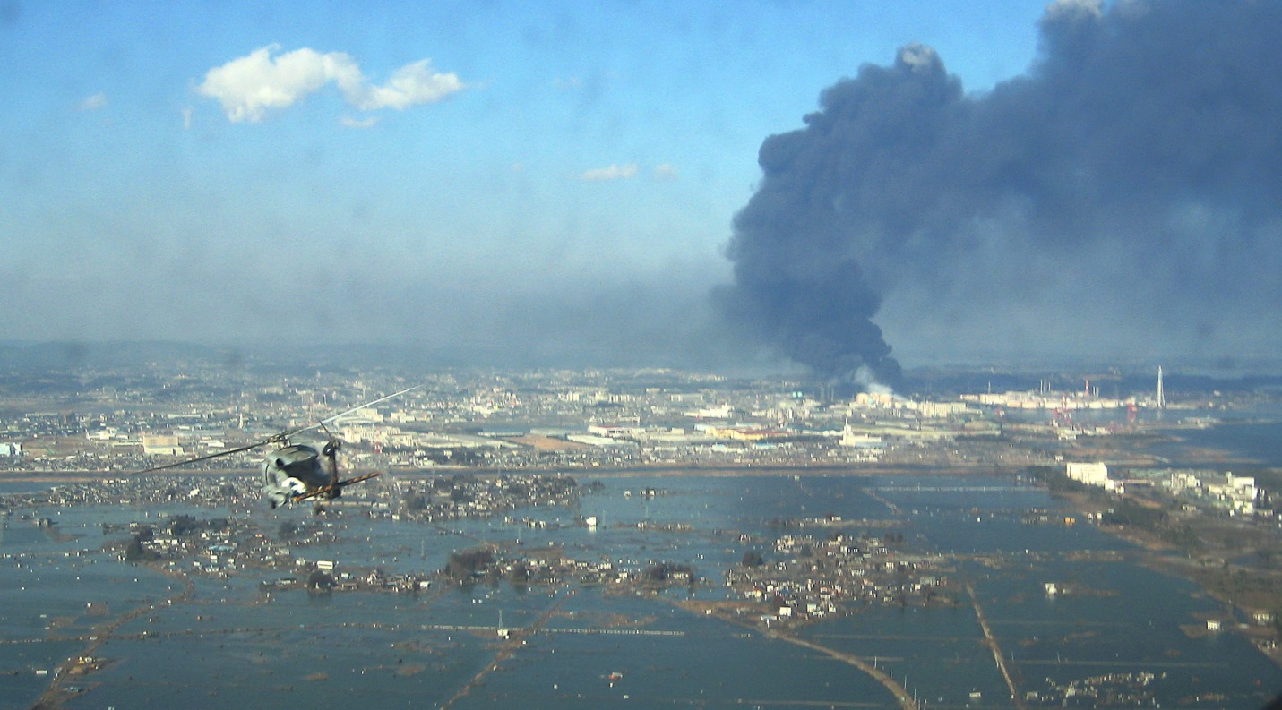
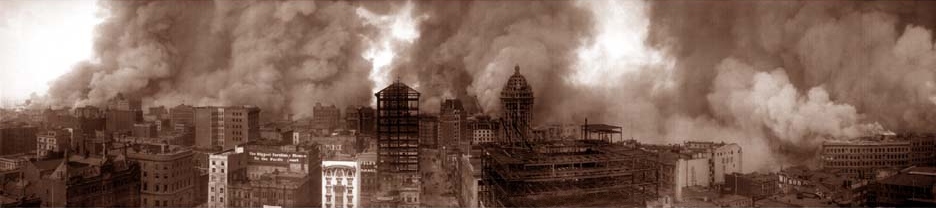
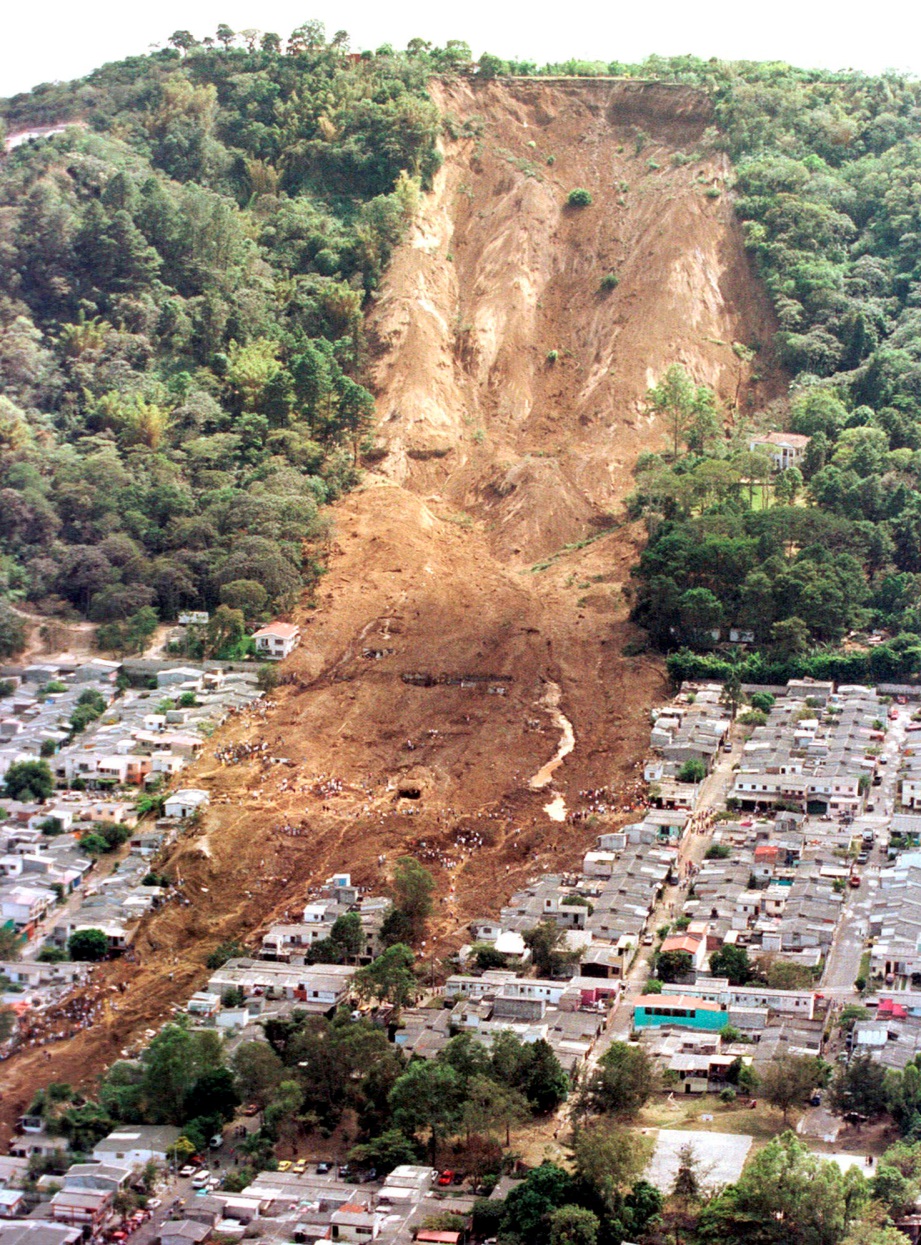

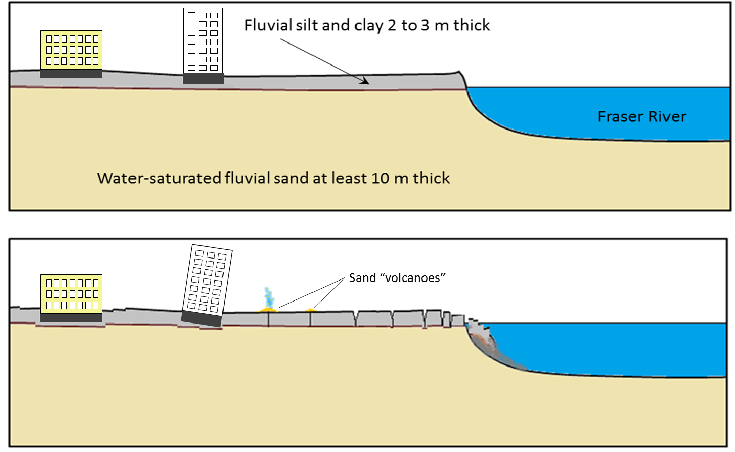
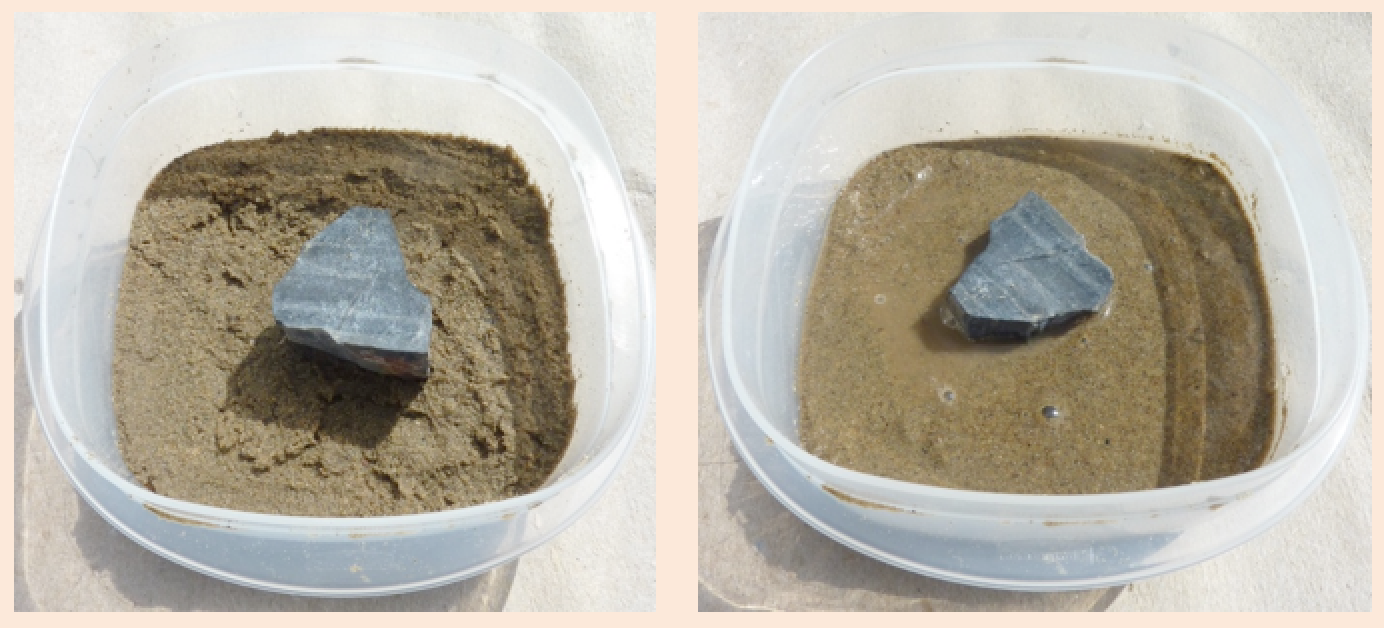
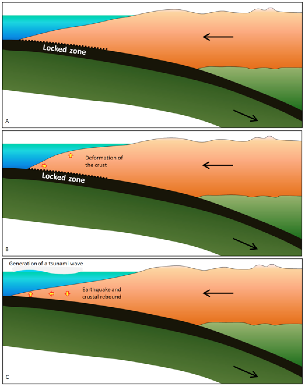
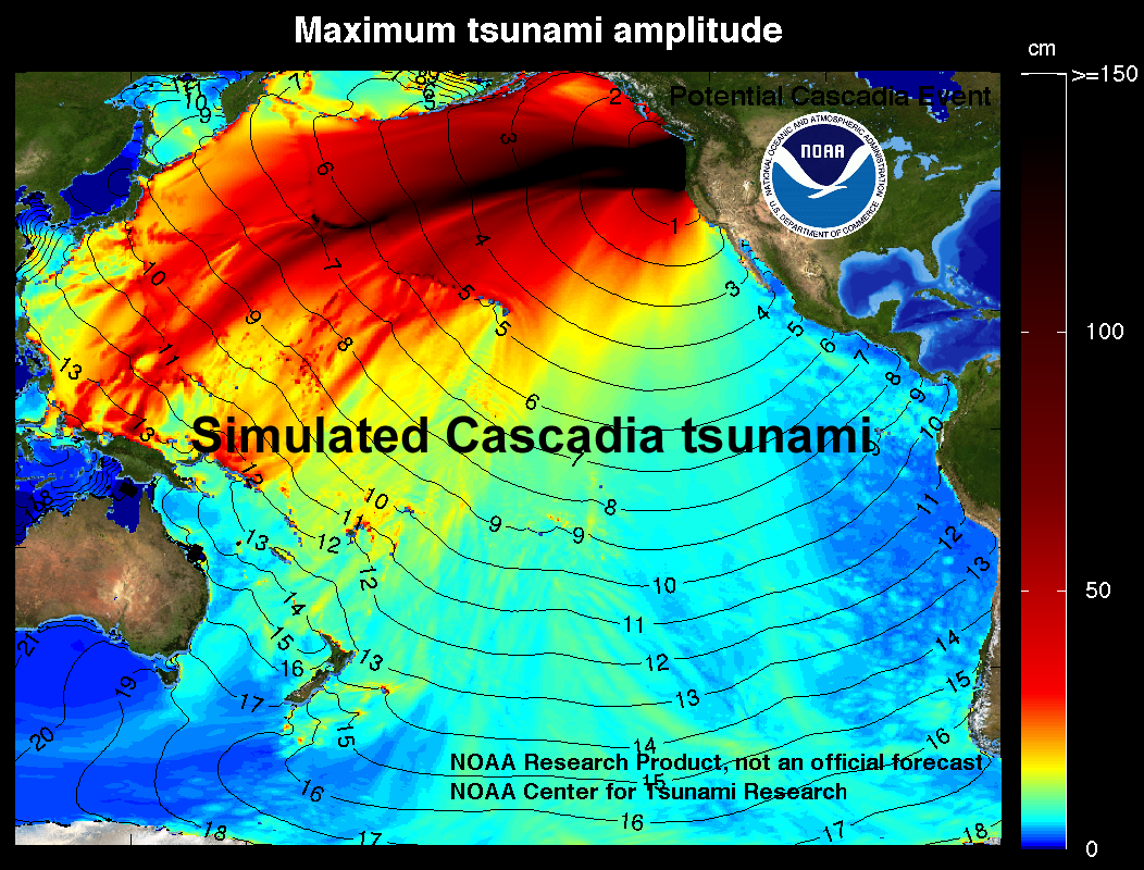

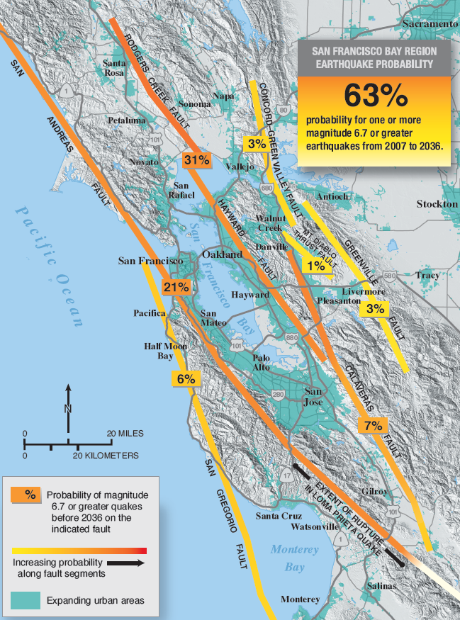

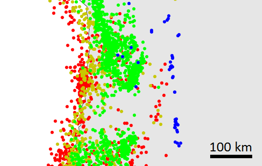
![Figure 12.1 Folds in sedimentary rocks near to Golden and the Kickinghorse River, BC. [SE]](http://opentextbc.ca/geology/wp-content/uploads/sites/110/2015/08/sedimentary-rocks.jpg)
![Figure 12.2 Depiction of the stress applied to rocks within the crust. The stress can be broken down into 3 components. Assuming that we’re looking down in this case, the green arrows represent north-south stress, the red arrows east-west stress, and the blue arrows (the one underneath is not visible) represent up-down stress. On the left all of the stress components are the same. On the right the north-south stress is least and the up-down stress is greatest. [SE]](http://opentextbc.ca/geology/wp-content/uploads/sites/110/2015/08/stress-applied-to-rocks-within-the-crust.png)
![Figure 12.3 The varying types of response of geological materials to stress. The straight dashed parts are elastic strain and the curved parts are plastic strain. In each case the X marks where the material fractured. A, the strongest material deforms relatively little and breaks at a high stress level. B, strong but brittle, shows no plastic deformation and breaks after relatively little elastic deformation. C, the most deformable, only breaks after significant elastic and plastic strain. The three deformation diagrams on the right show A and C before breaking and B after breaking. [SE]](http://opentextbc.ca/geology/wp-content/uploads/sites/110/2015/08/response-of-geological-materials-to-stress.png)
![Figure 12.4 Rock structures caused by various types of strain within rocks that have been stressed [all by SE]](https://opentextbc.ca/physicalgeologyearle/wp-content/uploads/sites/145/2016/03/structures-2.png)
![Figure 12.5 Examples of different types of folds and fold nomenclature. Axial planes are only shown for the anticlines, but synclines also have axial planes. [SE]](http://opentextbc.ca/geology/wp-content/uploads/sites/110/2015/08/folds-and-fold-nomenclature.png)
![Figure 12.6 An isoclinal recumbent fold [SE]](http://opentextbc.ca/geology/wp-content/uploads/sites/110/2015/08/isoclinal-recumbent-fold.png)
![Figure 12.7 Folded limestone (grey) and chert (rust-coloured) in Triassic Quatsino Fm. rocks on Quadra Island, BC. The image is about 1 m across. [SE]](http://opentextbc.ca/geology/wp-content/uploads/sites/110/2015/08/Triassic-Quatsino.jpg)
![Figure 12.8 Example of the topography in an area of folded rocks that has been eroded. In this case the blue and grey rocks are most resistant to erosion, and are represented by hills. [SE]](http://opentextbc.ca/geology/wp-content/uploads/sites/110/2015/08/topography-in-an-area-of-folded-rocks-that-has-been-eroded.png)

![Figure 12.9 Granite in the Coquihalla Creek area, B.C. (left) and sandstone at Nanoose, B.C. (right), both showing fracturing that has resulted from expansion due to removal of overlying rock. [SE]](https://opentextbc.ca/physicalgeologyearle/wp-content/uploads/sites/145/2016/03/fractures-2.png)
![Figure 12.10 A depiction of joints developed in the hinge area of folded rocks. Note that in this situation some rock types are more likely to fracture than others. [SE]](http://opentextbc.ca/geology/wp-content/uploads/sites/110/2015/08/depiction-of-joints.png)
![Figure 12.11 A depiction of joints developed in a rock that is under stress. [SE]](http://opentextbc.ca/geology/wp-content/uploads/sites/110/2015/08/joints-developed-in-a-rock.png)
![Figure 12.12 A fault (white dashed line) in intrusive rocks on Quadra Island, BC. The pink dike has been offset by the fault and the extent of the offset is shown by the white arrow (approx. 10 cm). Because the far side of the fault has move to the right, this is a right-lateral fault. If the photo was taken from the other side of the fault, it would still appear to have a right-lateral offset. [SE]](http://opentextbc.ca/geology/wp-content/uploads/sites/110/2015/08/intrusive-rocks-on-Quadra-Island.png)
![Figure 12.13 Depiction of reverse, normal and strike-slip faults. Reverse faults happen during compression while normal faults happen during extension. Most strike-slip faults are related to transform boundaries. [SE after: http://www.nature.nps.gov/geology/education/images/GRAPHICS/fault_types_2.jpg]](http://opentextbc.ca/geology/wp-content/uploads/sites/110/2015/08/reverse-normal-and-strike-slip-faults.png)
![Figure 12.14 Depiction of graben and horst structures that form in extensional situations. All of the faults are normal faults. [SE]](http://opentextbc.ca/geology/wp-content/uploads/sites/110/2015/08/graben-and-horst-structures.png)
![Figure 12.15 Depiction a thrust fault. Top: prior to faulting. Bottom: after significant fault offset. [SE]](https://opentextbc.ca/physicalgeologyearle/wp-content/uploads/sites/145/2016/03/thrust-2.png)
![Figure 12.16 Depiction of the McConnell Thrust in the eastern part of the Rockies. The rock within the faded area has been eroded. [SE]](http://opentextbc.ca/geology/wp-content/uploads/sites/110/2015/08/McConnell-Thrust.png)
![Figure 12.17 The McConnell Thrust at Mt. Yamnuska near to Exshaw, Alberta. Carbonate rocks (limestone) of Cambrian age have been thrust over top of Cretaceous mudstone. [SE]](http://opentextbc.ca/geology/wp-content/uploads/sites/110/2015/08/McConnell-Thrust-at-Mt.-Yamnuska.png)
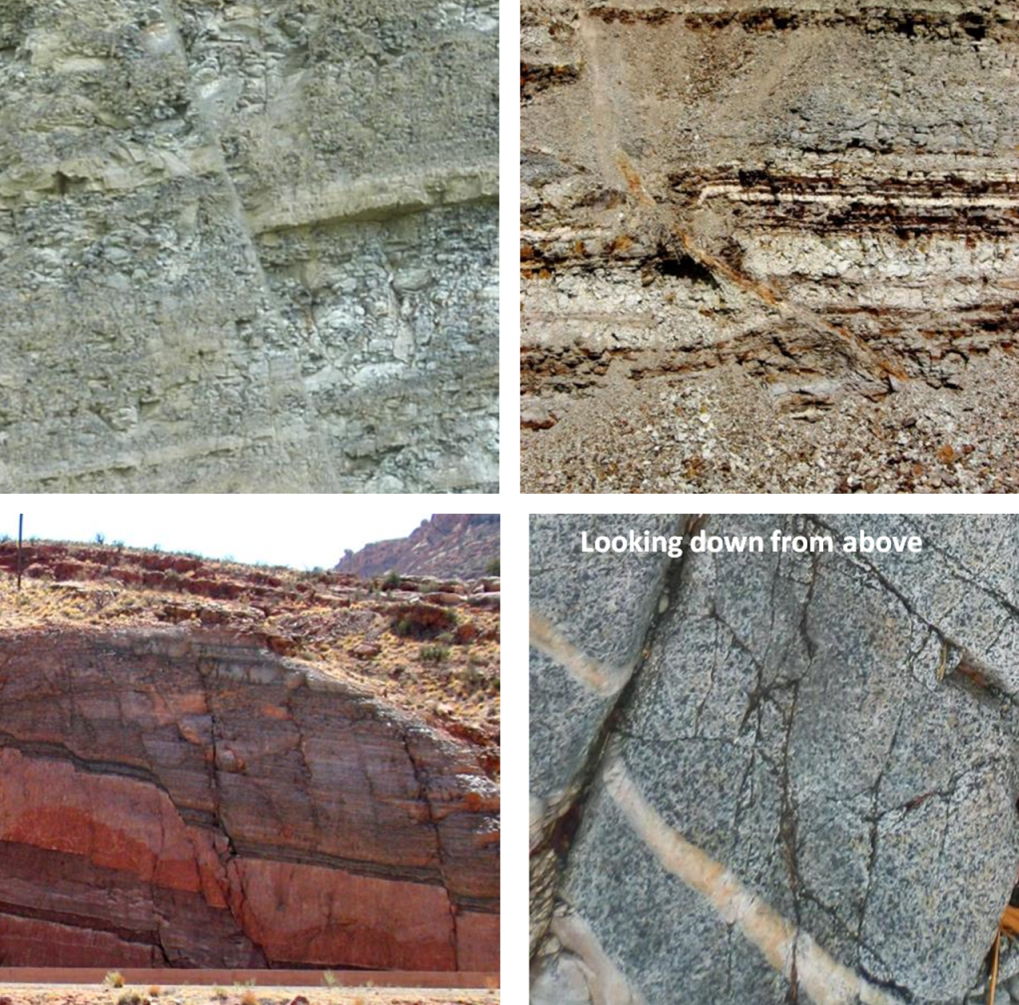
![Figure 12.18 A depiction of the strike and dip of some tilted sedimentary beds and the notation for expressing strike and dip on a map. [SE]](http://opentextbc.ca/geology/wp-content/uploads/sites/110/2015/08/strike-and-dip-of-some-tilted-sedimentary-beds.png)
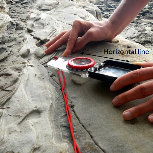
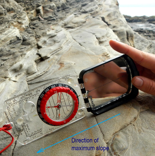
![Figure 12.20 A depiction of an anticline and a dyke in cross-section (looking from the side) and in map view (a.k.a. plan view) with the appropriate strike-dip and anticline symbols. [SE]](http://opentextbc.ca/geology/wp-content/uploads/sites/110/2015/08/anticline-and-a-dyke-in-cross-section.png)

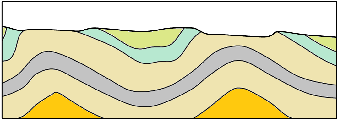
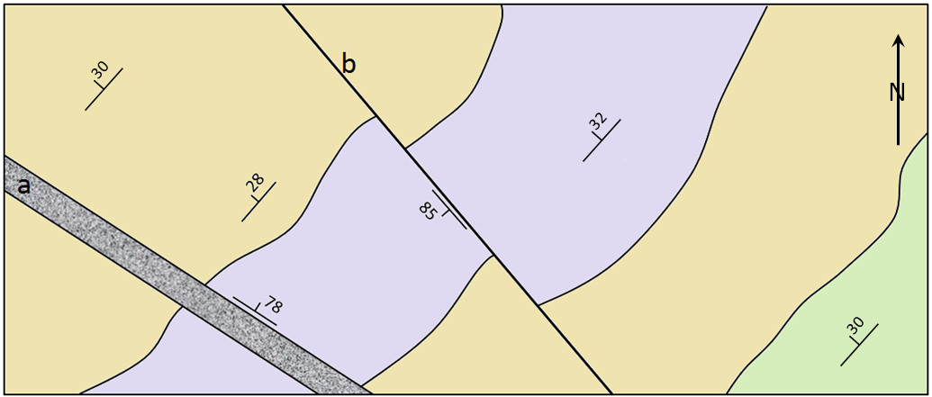
![Figure 13.1 A small waterfall on Johnston Creek in Johnston Canyon, Banff National Park, AB [SE]](http://opentextbc.ca/geology/wp-content/uploads/sites/110/2015/08/Johnston-Creek-.jpg)
![Figure 13.2 The various components of the water cycle. Black or white text indicates the movement or transfer of water from one reservoir to another. Yellow text indicates the storage of water. [SE after Wikipedia: http://upload.wikimedia.org/wikipedia/commons/5/54/Water_cycle_blank.svg]](http://opentextbc.ca/geology/wp-content/uploads/sites/110/2015/08/water-cycle.png)
![Figure 13.3a The storage reservoirs for water on Earth. Glacial ice is represented by the white band, groundwater the red band and surface water the very thin blue band at the top. The 0.001% stored in the atmosphere is not shown. [SE using data from: https://water.usgs.gov/edu/ watercyclefreshstorage.html]](http://opentextbc.ca/geology/wp-content/uploads/sites/110/2015/08/storage-reservoirs.png)
![Figure 13.3b Representation of the Earth’s water as a 1 L jug. The three drops represent all of the fresh water in lakes, streams and wetlands, plus all of the water in the atmosphere. [SE]](http://opentextbc.ca/geology/wp-content/uploads/sites/110/2015/08/Earth’s-water.png)
![Figure 13.4 Cawston Creek near Keremeos, B.C. The blue line shows the extent of the drainage basin. The dashed red line is the drainage basin of one of its tributaries. [SE]](https://opentextbc.ca/physicalgeologyearle/wp-content/uploads/sites/145/2016/06/cawston-2.png)
![Figure 13.5 Profile of the main stem of Cawston Creek near Keremeos, B.C. The maximum elevation of the drainage basin is about 1,840 m, near Mount Kobau. The base level is 275 m, at the Similkameen River. As shown, the gradient of the stream can be determined by dividing the change in elevation between any two points (rise) by the distance between those two points (run). [SE]](http://opentextbc.ca/geology/wp-content/uploads/sites/110/2015/08/Cawston-Creek-profile.png)
![Figure 13.6 The three drainage basins that are used for the Metro Vancouver water supply. [Used with permission of Metro Vancouver]](http://opentextbc.ca/geology/wp-content/uploads/sites/110/2015/08/three-drainage-basins.jpg)
![Figure 13.7 Typical dendritic, trellis, and rectangular stream drainage patterns. [SE]](http://opentextbc.ca/geology/wp-content/uploads/sites/110/2015/08/dendritic.png)
![Figure 13.8 Left: a typical deranged pattern; right: a typical radial drainage pattern developed around a mountain or hill. [SE]](https://opentextbc.ca/physicalgeologyearle/wp-content/uploads/sites/145/2016/06/deranged-radial-2.png)
![Figure 13.9 The topographic profile of a typical graded stream. [SE]](http://opentextbc.ca/geology/wp-content/uploads/sites/110/2015/08/typical-graded-stream.png)
![Figure 13.10 An example of a change in the base level of a small stream that flows into the Similkameen river near Keremeos. The previous base level was near the top of the sandy bank. The current base level is the river. [SE]](http://opentextbc.ca/geology/wp-content/uploads/sites/110/2015/08/Similkameen-river.jpg)
![Figure 13.11 Two streams with a lowered base level on the Juan de Fuca Trail, southwestern Vancouver Island. [SE]](https://opentextbc.ca/physicalgeologyearle/wp-content/uploads/sites/145/2016/06/jdf-waterfalls-2.png)
![Revelstoke Dam and Revelstoke Lake on the Columbia River at Revelstoke, BC [SE]](http://opentextbc.ca/geology/wp-content/uploads/sites/110/2015/08/Revelstoke-Dam-and-Revelstoke-Lake.jpg)
![Figure 13.12 Terraces on the Fraser River at High Bar. [Marie Betcher photo, used with permission]](http://opentextbc.ca/geology/wp-content/uploads/sites/110/2015/08/Fraser-River.jpg)
![Figure 13.13 A depiction of the Davis cycle of erosion: a: initial stage, b: youthful stage, c: mature stage, and d: old age. [SE]](http://opentextbc.ca/geology/wp-content/uploads/sites/110/2015/08/Davis-cycle-of-erosion.png)
![Figure 13.14 The relative velocity of stream flow depending on whether the stream channel is straight or curved (left), and with respect to the water depth (right). [SE]](https://opentextbc.ca/physicalgeologyearle/wp-content/uploads/sites/145/2016/06/meandering.png)
![Figure 13.15 Modes of transportation of sediments and dissolved ions (represented by red dots with + and – signs) in a stream. [SE]](http://opentextbc.ca/geology/wp-content/uploads/sites/110/2015/08/transportation-of-sediments.png)
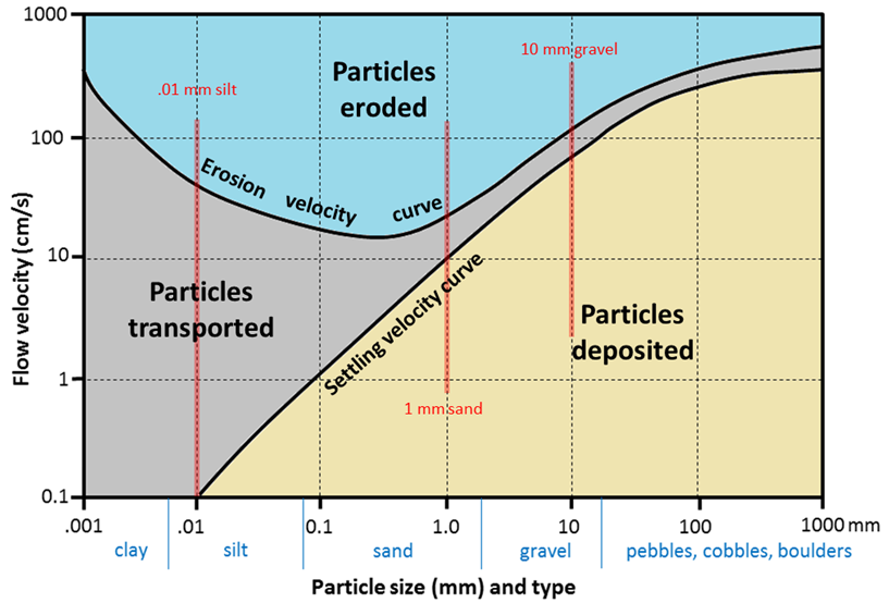
![Figure 13.17 The development of natural levées during flooding of a stream. The sediments of the levée become increasingly fine away from the stream channel, and even finer sediments — clay, silt, and fine sand — are deposited across most of the flood plain. [SE]](http://opentextbc.ca/geology/wp-content/uploads/sites/110/2015/08/natural-levées.png)
![Figure 13.18 The Cascade Falls area of the Kettle River, near Christina Lake, B.C. This stream has a step-pool morphology and a deep bedrock channel. [SE]](http://opentextbc.ca/geology/wp-content/uploads/sites/110/2015/08/Cascade-Falls-area.jpg)
![Figure 13.19 The braided channel of the Kicking Horse River at Field, B.C. [SE]](http://opentextbc.ca/geology/wp-content/uploads/sites/110/2015/08/Kicking-Horse-River.jpg)
![Figure 13.20 The braided Coldwater River, Mount St. Helens, Washington. [SE]](http://opentextbc.ca/geology/wp-content/uploads/sites/110/2015/08/Coldwater-River.jpg)
![Figure 13.21 The meandering channel of the Bonnell Creek, Nanoose, B.C. The stream is flowing toward the viewer. The sand and gravel point bar must have formed when the creek was higher and the flow faster than it was when the photo was taken. [SE]](http://opentextbc.ca/geology/wp-content/uploads/sites/110/2015/08/Bonnell-Creek.jpg)
![Figure 13.22 The meandering channel of the Nowitna River, Alaska. Numerous oxbow lakes are present and another meander cutoff will soon take place. [Oliver Kumis, http://commons.wikimedia.org/wiki/File:Nowitna_river.jpg]](http://opentextbc.ca/geology/wp-content/uploads/sites/110/2015/08/Nowitna-River.jpg)
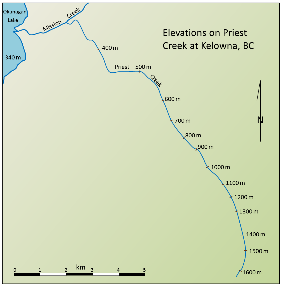
![Figure 13.23 The delta of the Fraser River and the plume of sediment that extends across the Strait of Georgia. The land outlined in red has formed over the past 10,000 years. [September 2011, SE after NASA: http://earthobservatory.nasa.gov/IOTD/view.php?id=77368]](http://opentextbc.ca/geology/wp-content/uploads/sites/110/2015/08/delta-of-the-Fraser-River.jpg)
![Figure 13.24 Variations in discharge of the Stikine River during 2013. [SE from data at Water Survey of Canada, Environment Canada, http://www.ec.gc.ca/rhc-wsc/]](http://opentextbc.ca/geology/wp-content/uploads/sites/110/2015/08/Stikine-River.png)
![Figure 13.25 Variations in discharge of the Qualicum River during 2013. [SE from data at Water Survey of Canada, Environment Canada, http://www.ec.gc.ca/rhc-wsc/]](http://opentextbc.ca/geology/wp-content/uploads/sites/110/2015/08/Qualicum-River.png)
![Figure 13.26 Map of the Red River Floodway around Winnipeg, Manitoba (left), and aerial view of the southern (inlet) end of the floodway (right). [Map from http://en.wikipedia.org/wiki/1997_Red_River_Flood#/media/File:Rednorthfloodwaymap.png and photo from Natural Resources Canada 2012, courtesy of the Geological Survey of Canada (Photo 2000-118 by G.R. Brooks).]](https://opentextbc.ca/physicalgeologyearle/wp-content/uploads/sites/145/2016/06/winnipeg-2.png)
![Figure 13.27 Map of the communities most affected by the 2013 Alberta floods (in orange) [SE]](http://opentextbc.ca/geology/wp-content/uploads/sites/110/2015/08/Alberta-floods.png)
![Figure 13.28 Flooding in Calgary (June 21, left) and Okotoks (June 20, right) during the 2013 southern Alberta flood [http://upload.wikimedia.org/wikipedia/commons/6/6a/Riverfront_Ave_Calgary_Flood_2013.jpg http://upload.wikimedia.org/wikipedia/en/9/9b/Okotoks_-_June_20%2C_2013_-_Flood_waters_in_local_campground_playground-03.JPG]](https://opentextbc.ca/physicalgeologyearle/wp-content/uploads/sites/145/2016/06/calgary-okotoks-2.png)
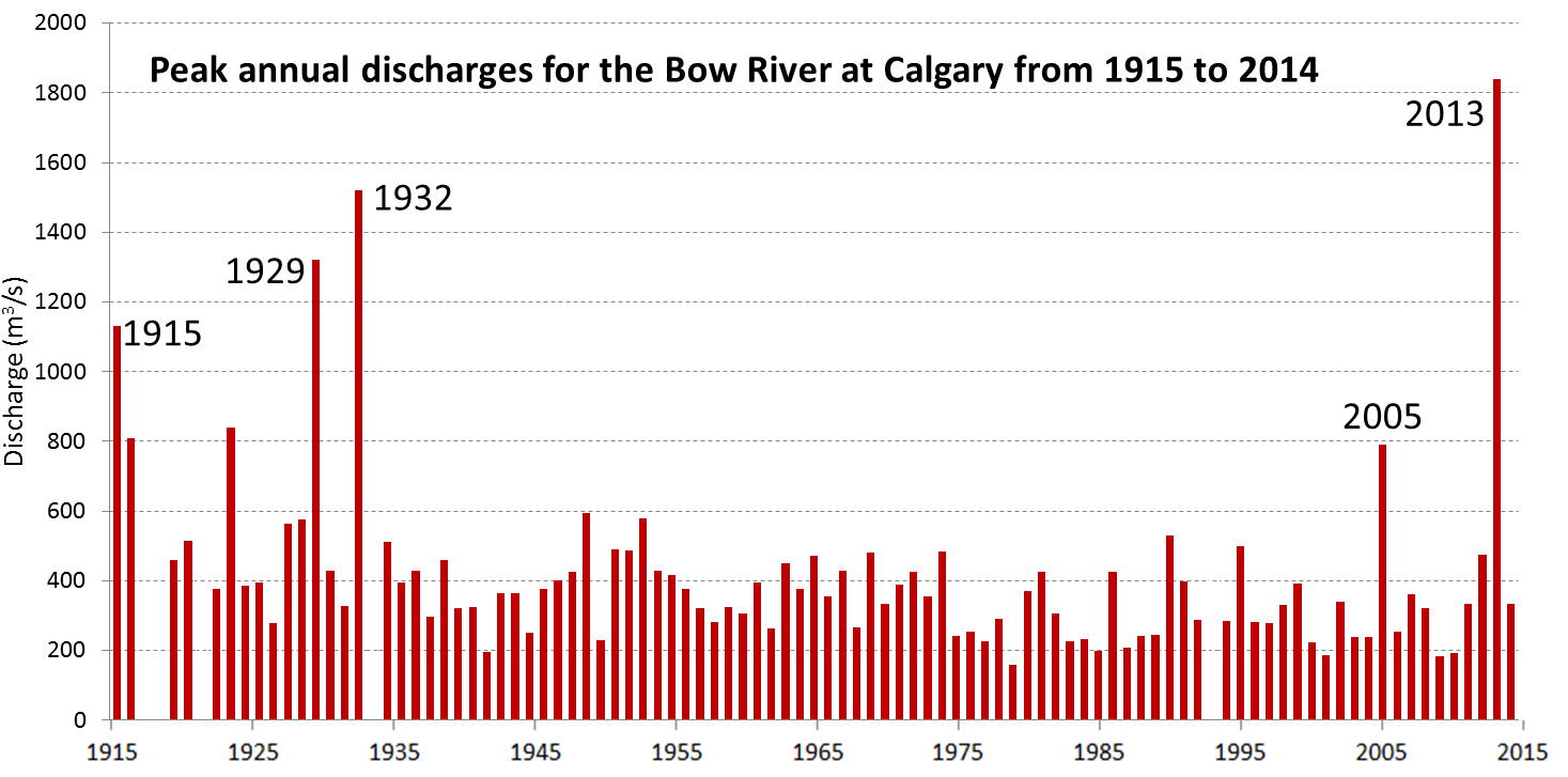
![Figure 14.1 A spring flowing from a limestone cave on Quadra Island, B.C. [SE]](http://opentextbc.ca/geology/wp-content/uploads/sites/110/2015/08/limestone-cave-on-Quadra-Island.jpg)
![Figure 14.2 Variations in porosity of unconsolidated materials (in red) and rocks (in blue) [SE]](http://opentextbc.ca/geology/wp-content/uploads/sites/110/2015/08/Variations-in-porosity.png)
![Figure 14.3 Variations in hydraulic conductivity (in metres/second) of unconsolidated materials (in red) and of rocks (in blue) [SE]](http://opentextbc.ca/geology/wp-content/uploads/sites/110/2015/08/Variations-in-hydraulic-conductivity.png)
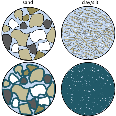
![Figure 14.4 A cross-section showing materials that might serve as aquifers and confining layers. The relative permeabilities are denoted by hydraulic conductivity (K = m/s). The pink rock is granite; the other layers are various sedimentary layers. [SE]](http://opentextbc.ca/geology/wp-content/uploads/sites/110/2015/08/aquifers-and-confining-layers.png)
![Figure 14.5 A depiction of the water table in cross-section, with the saturated zone below and the unsaturated zone above. The water table is denoted with a small upside-down triangle. [SE]](http://opentextbc.ca/geology/wp-content/uploads/sites/110/2015/08/water-table.png)
![Figure 14.6 A depiction of the water table and the potentiometric surface of a confined aquifer. [SE]](http://opentextbc.ca/geology/wp-content/uploads/sites/110/2015/08/water-table-and-the-potentiometric-surface.png)
![Figure 14.7 A perched aquifer above a regular unconfined aquifer. [SE]](http://opentextbc.ca/geology/wp-content/uploads/sites/110/2015/08/perched-aquifer.png)
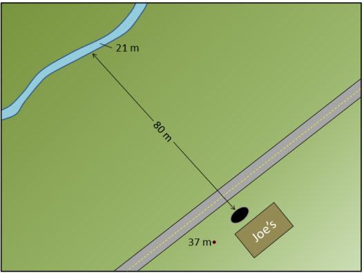
![Figure 14.8 Predicted equipotential lines (orange) and groundwater flow paths (blue) in an unconfined aquifer. The orange numbers are the elevations of the water table at the locations shown, and therefore they represent the pressure along the equipotential lines. [SE]](http://opentextbc.ca/geology/wp-content/uploads/sites/110/2015/08/unconfined-aquifer.png)
![Figure 14.9 Groundwater in a limestone karst region. The water in the caves above the water table does not behave like true groundwater because its flow is not controlled by water pressure, only by gravity. The water below the water table does behave like true groundwater. [SE]](http://opentextbc.ca/geology/wp-content/uploads/sites/110/2015/08/limestone-karst-region.png)
![Figure 14.10 A water-well drilling rig in operation in the Cassidy area, near Nanaimo, B.C. In the photo on the right the well is being test-pumped with air pressure. The casing (yellow arrow) is about 40 cm in diameter. [SE]](https://opentextbc.ca/physicalgeologyearle/wp-content/uploads/sites/145/2016/03/well-drilling-2.png)

![Figure 14.12 A similar scenario to that in Figure 14.11, but in this case, wells B and C have been pumped unsustainably for a long time. The cone of depression from well C has reached well B and has contributed to it going dry. [SE]](http://opentextbc.ca/geology/wp-content/uploads/sites/110/2015/08/cone-of-depression.png)
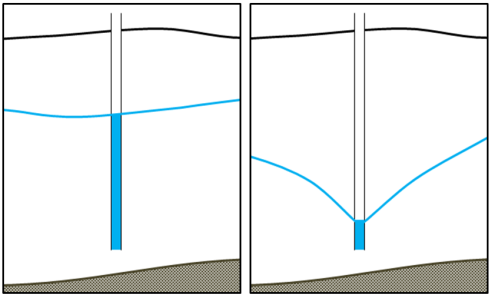
![Figure 14.13 B.C. observation well 232 near Cassidy Airport, Vancouver Island. The installation also has a solar panel, which is not visible in this view. [SE]](https://opentextbc.ca/physicalgeologyearle/wp-content/uploads/sites/145/2016/03/obs-well-2.png)
![Figure 14.14 Water level data for B.C. observation well 232 on Harby Rd., Lantzville, Vancouver Island. From 1979 to 2003, depths were recorded monthly. Automated equipment was installed in 2003, and the depths were recorded hourly since that time. [SE from data at: http://www.env.gov.bc.ca/wsd/data_searches/obswell/map/]](http://opentextbc.ca/geology/wp-content/uploads/sites/110/2015/08/Water-level-data-for-B.C.-observation-well.png)
![Figure 14.15 Water level data for B.C. observation well 232 for the period 1996 to 2000, showing seasonal variations [SE from data at: http://www.env.gov.bc.ca/wsd/data_searches/obswell/map/]](http://opentextbc.ca/geology/wp-content/uploads/sites/110/2015/08/1996-to-2000.png)
![Figure 14.16 Changes in water levels in wells in California over the period from 2011 to 2013 [SE from State of California Department of Water Resources data]](http://opentextbc.ca/geology/wp-content/uploads/sites/110/2015/08/Changes-in-water-levels.png)
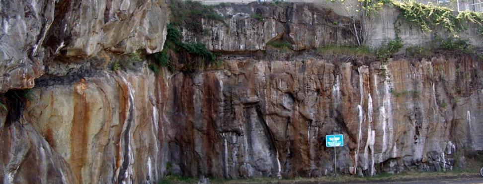
![Figure 14.18 The distribution of arsenic in groundwater in Bangladesh. The WHO recommended safe level for arsenic is 10 μg/L. All of the green, orange, and red areas on the map exceed that limit. [From: BGS and DPHE. 2001. Arsenic contamination of groundwater in Bangladesh. Kinniburgh, D G and Smedley, P L (Editors). British Geological Survey Technical Report WC/00/19. British Geological Survey: Keyworth. (http://www.bgs.ac.uk/arsenic/bangladesh/) ]](http://opentextbc.ca/geology/wp-content/uploads/sites/110/2015/08/distribution-of-arsenic.png)
![Figure 14.19 The vulnerability to anthropogenic contamination of aquifers on southern Vancouver Island. Much of the island is not mapped (shown as white) because of a lack of aquifer information in areas without wells. [From: Newton, P. and Gilchrist, A. 2010. Technical summary of intrinsic vulnerability mapping methods of Vancouver Island, Vancouver Island Water Resources Vulnerability Mapping Project, Vancouver Island University, 45pp. Used with permission. https://web.viu.ca/groundwater/PDF/VI_DRASTIC_Summary_Phase2_2010.pdf]](http://opentextbc.ca/geology/wp-content/uploads/sites/110/2015/08/anthropogenic-contamination.png)
![Figure 14.20 A cross-section of a typical modern landfill [SE]](http://opentextbc.ca/geology/wp-content/uploads/sites/110/2015/08/typical-modern-landfill.png)
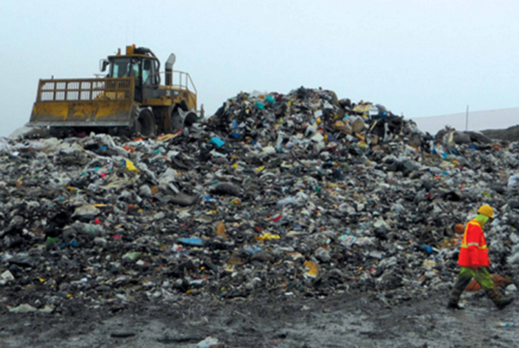
![Figure 14.21 The Trail lead-zinc smelter in 1929 [http://upload.wikimedia.org /wikipedia/commons/2/20 /Trail_Smelter_in_Year_1929.png]](http://opentextbc.ca/geology/wp-content/uploads/sites/110/2015/08/lead-zinc-smelter.png)
![Figure 14.22 Acidic runoff at the abandoned Mt. Washington Mine near Courtenay, B.C. [SE]](http://opentextbc.ca/geology/wp-content/uploads/sites/110/2015/08/Acidic-runoff.jpg)
![Figure 14.23 A closed and fenced gas station site in Nanaimo, B.C. The white pipes in the background are wells for monitoring groundwater contamination on the site. [SE]](http://opentextbc.ca/geology/wp-content/uploads/sites/110/2015/08/fenced-gas-station-site.jpg)
![Figure 14.24 A depiction of the fate of different components of a petroleum spill from an underground storage tank. [SE]](http://opentextbc.ca/geology/wp-content/uploads/sites/110/2015/08/petroleum-spill.png)
![Figure 14.25 A typical septic system. [SE]](http://opentextbc.ca/geology/wp-content/uploads/sites/110/2015/08/septic-system.png)
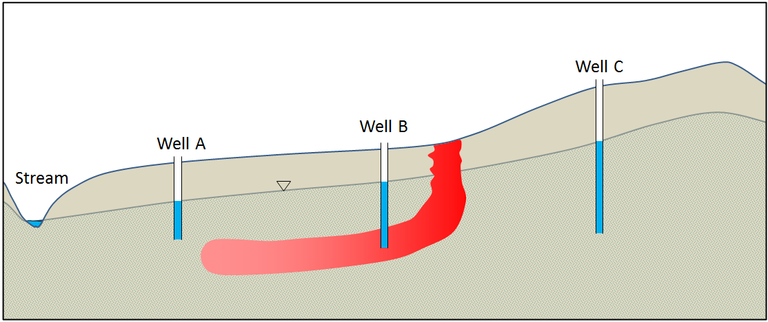
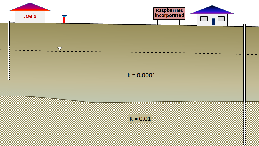
![Photograph of the site of the 1965 Hope Slide as seen in 2014. The initial failure is thought to have taken place along the foliation planes and sill within the area shown in the inset. [SE]](http://opentextbc.ca/geology/wp-content/uploads/sites/110/2015/08/1965-Hope-Slide-as-seen-in-2014.png)
![Figure 15.2 Differences in the shear and normal components of the gravitational force on slopes with differing steepness. The gravitational force is the same in all three cases. In (a) the shear force is substantially less than the shear strength, so the block should be stable. In (b) the shear force and shear strength are about equal, so the block may or may not move. In (c) the shear force is substantially greater than the shear strength, so the block is very likely to move. [SE]](http://opentextbc.ca/geology/wp-content/uploads/sites/110/2015/08/Differences-in-the-shear-and-normal-components.png)
![Relative stability of slopes as a function of the orientation of weaknesses (in this case bedding planes) relative to the slope orientations. [SE]](http://opentextbc.ca/geology/wp-content/uploads/sites/110/2015/08/Relative-stability-of-slopes-as-a-function-of-the-orientation-of-weaknesses.png)
![Figure 15.4 Left: Glacial outwash deposits at Point Grey, in Vancouver. The dark lower layer is made up of sand, silt, and clay. The light upper layer is well-sorted sand. Right: Glacial till on Quadra Island, B.C. The till is strong enough to have formed a near-vertical slope. [SE]](https://opentextbc.ca/physicalgeologyearle/wp-content/uploads/sites/145/2016/06/quadra-sand-2.png)
![Depiction of dry, moist, and saturated sand [SE]](http://opentextbc.ca/geology/wp-content/uploads/sites/110/2015/08/Depiction-of-dry-moist-and-saturated-sand.png)
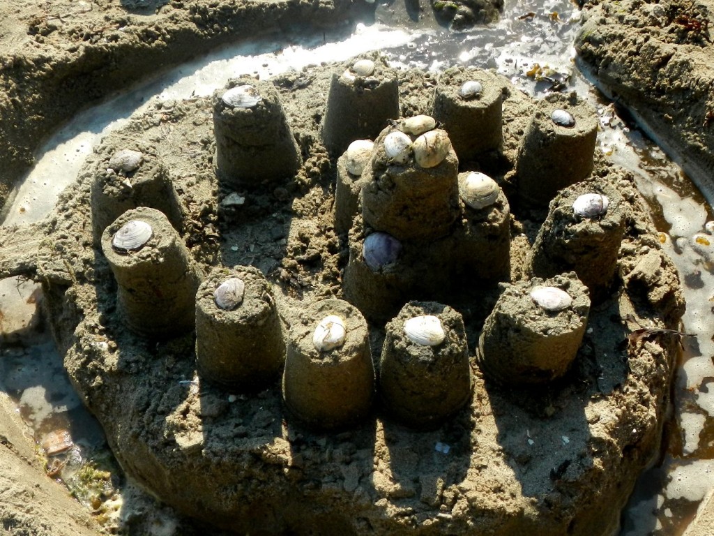
![Figure 15.6 The debris flow in the Riverside Drive area of North Vancouver in January, 2005 happened during a rainy period, but was likely triggered by excess runoff related to the roads at the top of this slope and by landscape features, including a pool, in the area surrounding the house visible here. [The Province, used with permission]](http://opentextbc.ca/geology/wp-content/uploads/sites/110/2015/08/debris-flow-in-the-Riverside-Drive-area-of-North-Vancouver-.jpg)
![Figure 15.7 The contribution of freeze-thaw to rock fall [SE]](http://opentextbc.ca/geology/wp-content/uploads/sites/110/2015/08/contribution-of-freeze-thaw-to-rock-fall.png)
![Figure 15.8 Left: A talus slope near Keremeos, B.C., formed by rock fall from the cliffs above. Right: The results of a rock fall onto a highway west of Keremeos in December 2014. [SE]](https://opentextbc.ca/physicalgeologyearle/wp-content/uploads/sites/145/2016/06/keremeos-2.png)
![Figure 15.9 The Downie Slide, a sackung, on the shore of the Revelstoke Reservoir (above the Revelstoke Dam). The head scarp is visible at the top and a side-scarp along the left side. [from Google Earth]](http://opentextbc.ca/geology/wp-content/uploads/sites/110/2015/08/The-Downie-Slide.png)
![Figure 15.10 Site of the 2008 rock slide at Porteau Cove. Notice the prominent fracture set parallel to the surface of the slope. The slope has been stabilized with rock bolts (top) and holes have been drilled into the rock to improve drainage (one is visible in the lower right). Risk to passing vehicles from rock fall has been reduced by hanging mesh curtains (background). [SE photo 2012]](http://opentextbc.ca/geology/wp-content/uploads/sites/110/2015/08/Site-of-the-2008-rock-slide-at-Porteau-Cove.jpg)
![Figure 15.11 The 2010 Mt. Meager rock avalanche, showing where the slide originated (arrow, 4 km upstream). It then raced down a steep narrow valley, and out into the wider valley in the foreground. [Mika McKinnon photo, http://www.geomika.com/blog/2011/01/05/the-trouble-with-landslides/ Used with permission.]](http://opentextbc.ca/geology/wp-content/uploads/sites/110/2015/08/2010-Mt.-Meager-rock-avalanche-.png)
![Figure 15.12 A depiction of the contribution of freeze-thaw to creep. The blue arrows represent uplift caused by freezing in the wet soil underneath, while the red arrows represent depression by gravity during thawing. The uplift is perpendicular to the slope, while the drop is vertical. [SE]](http://opentextbc.ca/geology/wp-content/uploads/sites/110/2015/08/depiction-of-the-contribution-of-freeze-thaw.png)
![Figure 15.13 Evidence of creep (tilted grave markers) at a cemetery in Nanaimo, BC [SE]](http://opentextbc.ca/geology/wp-content/uploads/sites/110/2015/08/Evidence-of-creep.jpg)
![Figure 15.14 A depiction of the motion of unconsolidated sediments in an area of slumping [SE]](http://opentextbc.ca/geology/wp-content/uploads/sites/110/2015/08/motion-of-unconsolidated-sediments-in-an-area-of-slumping-.png)
![Figure 15.15 A slump along the banks of a small coulee near Lethbridge, Alberta. The main head-scarp is clearly visible at the top, and a second smaller one is visible about one-quarter of the way down. The toe of the slump is being eroded by the seasonal stream that created the coulee. [SE 2005]](http://opentextbc.ca/geology/wp-content/uploads/sites/110/2015/08/slump-along-the-banks-of-a-small-coulee-near-Lethbridge.jpg)
![Figure 15.16 A slump (left) and an associated mudflow (centre) at the same location as Figure 15.15, near Lethbridge, Alberta. [SE]](https://opentextbc.ca/physicalgeologyearle/wp-content/uploads/sites/145/2016/06/lethbridge-2.png)
![Figure 15.17 The lower part of debris flow within a steep stream channel near Buttle Lake, B.C., in November 2006. [SE]](https://opentextbc.ca/physicalgeologyearle/wp-content/uploads/sites/145/2016/06/buttle.png)
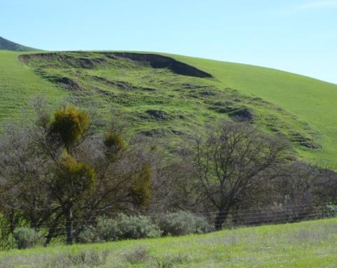
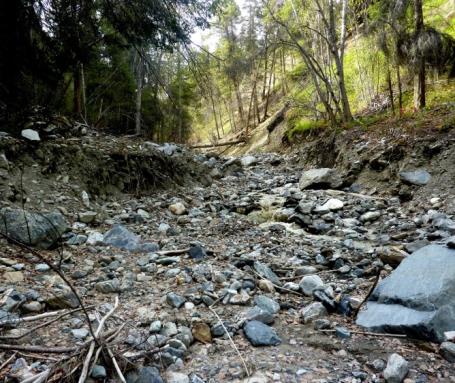
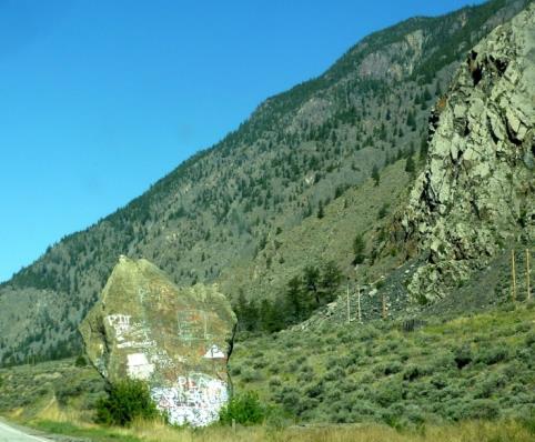
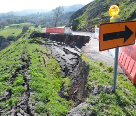
![Figure 15.18 An example of a road constructed by cutting into a steep slope and the use of the cut material as fill. [SE]](http://opentextbc.ca/geology/wp-content/uploads/sites/110/2015/08/road-constructed-by-cutting-into-a-steep-slope.png)
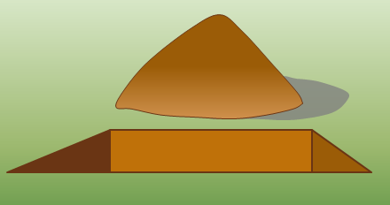
![Figure 15.19 Part of a motion-monitoring device at the Checkerboard Slide near Revelstoke, B.C. The lower end of the cable is attached to a block of rock that is unstable. Any incremental motion of that block will move the cable and this will be detectable on this device. [SE]](http://opentextbc.ca/geology/wp-content/uploads/sites/110/2015/08/motion-monitoring-device-at-the-Checkerboard-Slide-near-Revelstoke.jpg)
![Figure 15.20 Mount Rainier, Washington, from Tacoma. [By Lynn Topinka, US Geological Survey, http://en.wikipedia.org/wiki/Mount_ Rainier#/media/File:Mount_Rainier_over_Tacoma.jpg]](http://opentextbc.ca/geology/wp-content/uploads/sites/110/2015/08/Mount-Rainier.jpg)
![Figure 15.21 A snow avalanche shelter on the Coquihalla Highway. The expected path of the avalanche is the steep un-treed slope above. [SE]](https://opentextbc.ca/physicalgeologyearle/wp-content/uploads/sites/145/2016/06/snow-shed-2.png)
![Figure 15.22 Two strategies for mitigating debris flows on the Sea-to-Sky Highway. Left: A concrete –lined channel on Alberta Creek allows debris to flow quickly through to the ocean. Right: A debris-flow catchment basin on Charles Creek. In 2010, a debris flow filled the basin to the level of the dotted white line. [SE]](https://opentextbc.ca/physicalgeologyearle/wp-content/uploads/sites/145/2016/06/alberta-charles-2.png)
![Figure 15.23 The Barrier, south of Whistler, B.C., was the site of a huge rock avalanche in 1855, which extended from the cliff visible here 4 km down the valley and across the current location of the Sea-to-Sky Highway and the Cheakamus River. [SE]](http://opentextbc.ca/geology/wp-content/uploads/sites/110/2015/08/The-Barrier.jpg)
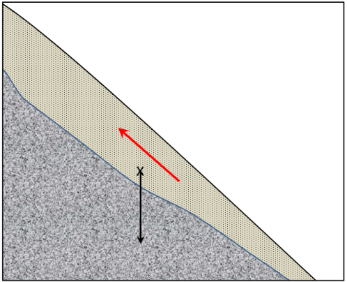
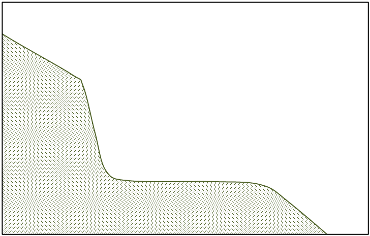
![Figure 16.1 Glaciers in the Alberta Rockies: Athabasca Glacier (centre left), Dome Glacier (right), and the Columbia Icefield (visible above both glaciers). The Athabasca Glacier has prominent lateral moraines on both sides. [SE]](https://opentextbc.ca/physicalgeologyearle/wp-content/uploads/sites/145/2016/03/athabasca-2.png)
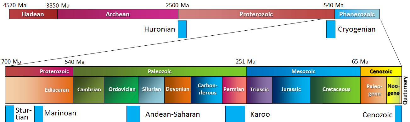
![Figure 16.3 The global temperature trend over the past 65 Ma (the Cenozoic). From the end of the Paleocene to the height of the Pleistocene Glaciation, global average temperature dropped by about 14°C. (PETM is the Palecene-Eocene thermal maximum) [SE after Routledge, 2013, http://www.alpineanalytics.com/Climate/DeepTime.html ]](https://opentextbc.ca/physicalgeologyearle/wp-content/uploads/sites/145/2016/03/cenozoic-t-2.png)
![Figure 16.4 The Antarctic Circumpolar Current (red arrows) prevents warm water from the rest of Earth’s oceans from getting close to Antarctica. [SE]](http://opentextbc.ca/geology/wp-content/uploads/sites/110/2015/07/Antarctic-Circumpolar.png)
![Figure 16.5 Foram oxygen isotope record for the past 5 million years based on O isotope data from sea-floor sediments. [created by SE using from data at http://www.lorraine-lisiecki.com/stack.html, Lisiecki and Raymo, 2005]](http://opentextbc.ca/geology/wp-content/uploads/sites/110/2015/07/Foram-oxygen-isotope-record.png)
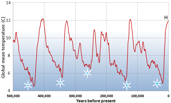
![Figure 16.6 The extent of the Cordilleran and Laurentide Ice Sheets near the peak of the Wisconsin Glaciation, around 15 ka. [re-drawn by SE based on a map at: https://www.ncdc.noaa.gov/paleo/glaciation.html]](http://opentextbc.ca/geology/wp-content/uploads/sites/110/2015/07/Cordilleran-and-Laurentide-Ice-Sheets.png)
![Figure 16.7 Part of the continental ice sheet in Greenland, with some outflow alpine glaciers in the foreground. [SE]](http://opentextbc.ca/geology/wp-content/uploads/sites/110/2015/07/Greenland.jpg)
![Figure 16.8 Simplified cross-sectional profiles the continental ice sheets in Greenland and Antarctica – both drawn to the same scale. [SE]](https://opentextbc.ca/physicalgeologyearle/wp-content/uploads/sites/145/2016/03/antarctic-greenland-2.png)
![Figure 16.9 Schematic ice-flow diagram for the Antarctic Ice Sheet. [SE]](https://opentextbc.ca/physicalgeologyearle/wp-content/uploads/sites/145/2016/06/antarctic-flow-2.png)
![Figure 16.10 Schematic ice-flow diagram for an alpine glacier. [SE]](https://opentextbc.ca/physicalgeologyearle/wp-content/uploads/sites/145/2016/03/ice-flow-2.png)
![Figure 16.11 Steps in the process of formation of glacial ice from snow, granules, and firn. [SE]](http://opentextbc.ca/geology/wp-content/uploads/sites/110/2015/07/formation-of-glacial-ice.png)
![Figure 16.12 The approximate location of the equilibrium line (red) in September 2013 on the Overlord Glacier, near Whistler, B.C. [SE, after Isaac Earle, used with permission]](http://opentextbc.ca/geology/wp-content/uploads/sites/110/2015/07/equilibrium-line.png)
![Figure 16.13 Stress within a valley glacier (red numbers) as determined from the slope of the ice surface and the depth within the ice. The ice will deform and flow where the stress is greater than 100 kilopascals, and the relative extent of that deformation is depicted by the red arrows. Any deformation motion in the lower ice will be transmitted to the ice above it, so although the red arrows get shorter toward the top, the ice velocity increases upward (blue arrows). The upper ice (above the red dashed line) does not flow, but it is pushed along with the lower ice. [SE]](https://opentextbc.ca/physicalgeologyearle/wp-content/uploads/sites/145/2016/03/ice-stress-2.png)
![Figure 16.14 Crevasses on Overlord Glacier in the Whistler area, B.C. [Isaac Earle, used with permission]](http://opentextbc.ca/geology/wp-content/uploads/sites/110/2015/07/Overlord-Glacier.jpg)
![Figure 16.15 Differences in glacial ice motion with basal sliding (left) and without basal sliding (right). The dashed red line indicates the upper limit of plastic internal flow. [SE]](https://opentextbc.ca/physicalgeologyearle/wp-content/uploads/sites/145/2016/03/flow-rates-2.png)
![Figure 16.16 Thrust faults at the leading edge of the Athabasca Glacier, Alberta. The arrows show how the trailing ice has been thrust over the leading ice. (The dark vertical stripes are mud from sediments that have been washed off of the lateral moraine lying on the surface of the ice.) [SE]](https://opentextbc.ca/physicalgeologyearle/wp-content/uploads/sites/145/2016/03/thrusting-2.png)
![Figure 16.17 Markers on an alpine glacier move forward over a period of time. [SE]](https://opentextbc.ca/physicalgeologyearle/wp-content/uploads/sites/145/2016/03/flow-before-after-2.png)
![Figure 16.18 Mt. Robson, the tallest peak in the Canadian Rockies, Berg Glacier (centre), and Berg Lake. Although there were no icebergs visible when this photo was taken, the Berg Glacier loses mass by shedding icebergs into Berg Lake. [SE]](http://opentextbc.ca/geology/wp-content/uploads/sites/110/2015/07/Mt.-Robson.jpg)
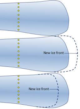
![Figure 16.19 Drumlins — streamlined hills formed beneath a glacier, here made up of sediment — in the Amundsun Gulf region of Nunavut. The drumlins are tens of metres high, a few hundred metres across and a few kilometres long. One of them is highlighted with a dashed white line. [http://earthobservatory.nasa.gov/IOTD/view.php?id=85506]](http://opentextbc.ca/geology/wp-content/uploads/sites/110/2015/07/Drumlins-e1438086592891.png)
![Figure 16.20 A depiction of a U-shaped valley occupied by a large glacier. [SE]](https://opentextbc.ca/physicalgeologyearle/wp-content/uploads/sites/145/2016/03/u-valley-2.png)
![Figure 16.21 The view down the U-shaped valley of Mill Creek valley toward the U-shaped valley of Howe Sound, with the village of Britannia on the opposite side. [http://commons.wikimedia.org/wiki/File:Woodf1a.jpg]](http://opentextbc.ca/geology/wp-content/uploads/sites/110/2015/07/Mill-Creek-valley.jpg)
![Figure 16.22 A view from the International Space Station of the Swiss Alps in the area of the Aletsch Glacier. The prominent peaks labelled “Horn” are the Eiger (left) and Wetterhorn (right). A variety of alpine glacial erosion features are labelled. [SE after http://earthobservatory.nasa.gov/IOTD/view.php?id=7195]](https://opentextbc.ca/physicalgeologyearle/wp-content/uploads/sites/145/2016/03/aletsch-2.png)
![Figure 16.23 A diagram of some of the important alpine-glaciation erosion features. [SE after http://commons.wikimedia.org/wiki/ File:Glacial_landscape_LMB.png]](http://opentextbc.ca/geology/wp-content/uploads/sites/110/2015/07/alpine-glaciation-erosion.png)
![[SE after http://en.wikipedia.org/wiki/Mount_Assiniboine#/media/File:Mount_Assiniboine_Sunburst_Lake.jpg]](http://opentextbc.ca/geology/wp-content/uploads/sites/110/2015/07/Glacial-Erosion-Features.png)
![Figure 16.24 Bowyer Island, a drumlin in Howe Sound, B.C. Ice flow was from right to left. [SE]](https://opentextbc.ca/physicalgeologyearle/wp-content/uploads/sites/145/2016/03/bowyer-2.png)
![Figure 16.25 Left: Roches moutonées with glacial striae near Squamish, B.C. Right: Glacial striae at the same location near Squamish. Ice flow was from right to left in both cases. [SE]](https://opentextbc.ca/physicalgeologyearle/wp-content/uploads/sites/145/2016/03/squamish-2.png)
![Figure 16.26 Lower Thornton Lake, a tarn, in the Northern Cascades National Park, Washington. [http://commons.wikimedia.org/wiki/File:Trappers_Peak_and_lower_Thornton_Lake.jpg ]](http://opentextbc.ca/geology/wp-content/uploads/sites/110/2015/07/Lower-Thornton-Lake.jpg)
![Figure 16.27 Peyto Lake in the Alberta Rockies, is both a finger lake and a moraine lake as it is dammed by an end moraine, on the right. [http://commons.wikimedia.org/wiki/File:1_Peyto_lake_panorama_2006.jpg]](https://opentextbc.ca/physicalgeologyearle/wp-content/uploads/sites/145/2016/03/peyto-2.png)
![Figure 16.28 Potholes Coulee near Wenatchee, Washington, one of many basins that received Lake Missoula floodwaters during the late Pleistocene. Here the water flowed from right to left, over the cliff and into this basin. [SE]](http://opentextbc.ca/geology/wp-content/uploads/sites/110/2015/07/Potholes-Coulee.jpg)
![Figure 16.29 Part of the Bering Glacier in southeast Alaska, the largest glacier in North America. It is about 14 km across in the centre of this view. [http://water.usgs.gov/edu/gallery/glacier-satellite.html]](https://opentextbc.ca/physicalgeologyearle/wp-content/uploads/sites/145/2016/03/alaska-2.jpg)
![Figure 16.30 A depiction of the various types of sediments associated with glaciation. The glacier is shown in cross-section. [http://water.usgs.gov/edu/gallery/glacier-satellite.html]](https://opentextbc.ca/physicalgeologyearle/wp-content/uploads/sites/145/2016/03/glacier-cross-section-2.png)
![Figure 16.31 Examples of glacial till: a: lodgement till from the front of the Athabasca Glacier, Alberta; b: ablation till at the Horstman Glacier, Blackcomb Mountain, B.C. [SE]](https://opentextbc.ca/physicalgeologyearle/wp-content/uploads/sites/145/2016/03/till-2.png)
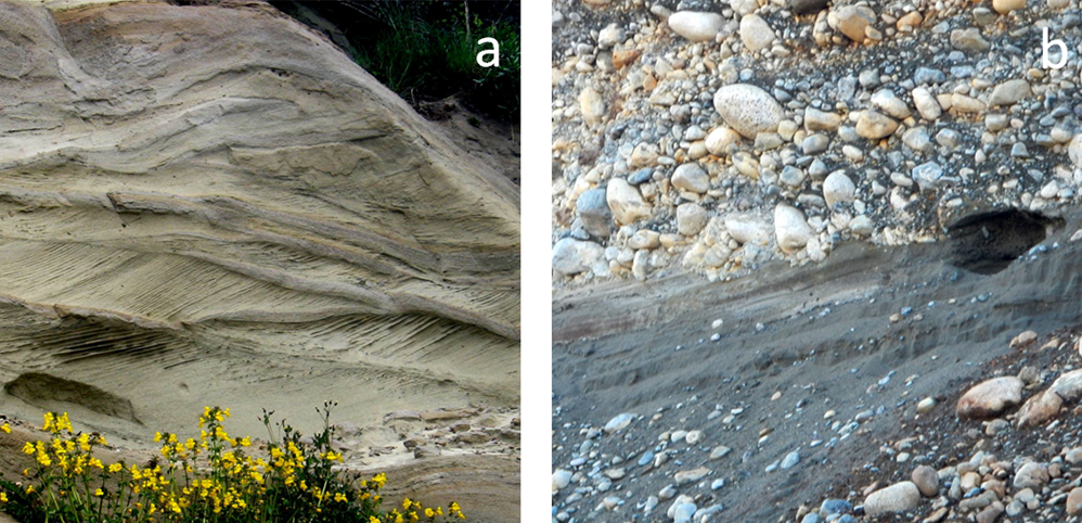
![Figure 16.33 A kettle lake amid vineyards and orchards in the Osoyoos area of B.C. [SE]](https://opentextbc.ca/physicalgeologyearle/wp-content/uploads/sites/145/2016/03/kettle-2.png)
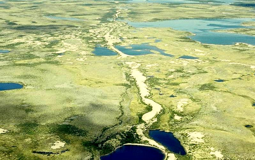
![Figure 16.35 Examples of glacial sediments formed in quiet water: a: glaciolacustrine sediment with a drop stone, Nanaimo, B.C.; and b: a laminated glaciomarine sediment, Englishman River, B.C. Although not visible in this photo, the glaciomarine sediment has marine shell fossils. [SE]](https://opentextbc.ca/physicalgeologyearle/wp-content/uploads/sites/145/2016/03/gl-gm-2.png)
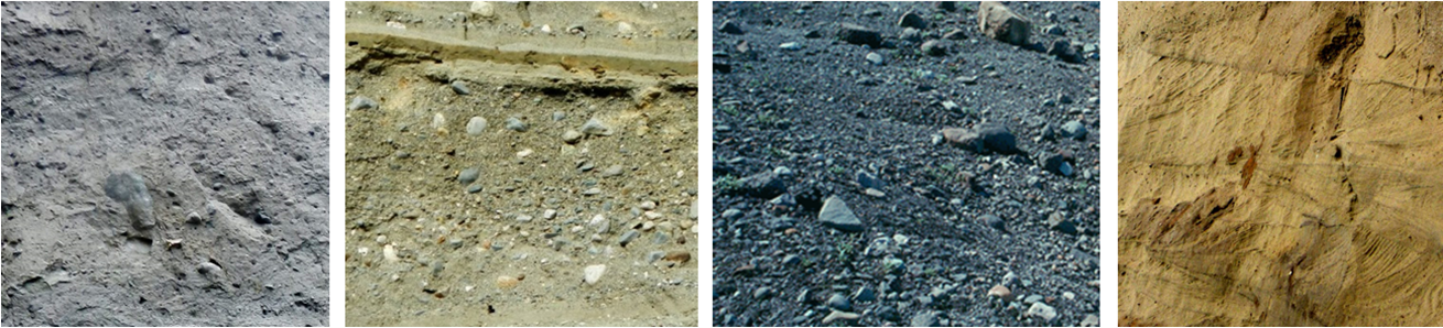
![Figure 17.1 Chesterman Beach near Tofino on the west coast Vancouver Island. The strip of sediment connecting the main beach to the rocky island is a tombolo. [Photo by Todd Byrnes, used with permission of Chesterman Beach B and B]](http://opentextbc.ca/geology/wp-content/uploads/sites/110/2015/08/Chesterman-Beach-near-Tofino.png)
![Figure 17.2 The parameters of water waves [SE]](http://opentextbc.ca/geology/wp-content/uploads/sites/110/2015/08/The-parameters-of-water-waves.png)
![Figure 17.3 The orbital motion of a parcel of water (black dot) as a wave moves across the surface. [SE]](http://opentextbc.ca/geology/wp-content/uploads/sites/110/2015/08/orbital-motion-of-a-parcel-of-water.png)
![Figure 17.4 The effect of waves approaching a sandy shore [SE]](http://opentextbc.ca/geology/wp-content/uploads/sites/110/2015/08/The-effect-of-waves-approaching-a-sandy-shore.png)
![Figure 17.5 Waves breaking on the shore at Greensand Beach, Hawaii (the sand is green because it is made up mostly of the mineral olivine eroded from the nearby volcanic rocks) [SE]](http://opentextbc.ca/geology/wp-content/uploads/sites/110/2015/08/Greensand-Beach.jpg)
![Figure 17.6 Waves approaching the shore of Long Beach in Pacific Rim National Park. As the waves (depicted by white lines) approach shore, they are refracted to become more parallel to the beach, and their wavelength decreases. [SE]](http://opentextbc.ca/geology/wp-content/uploads/sites/110/2015/08/Long-Beach-in-Pacific-Rim-National-Park.png)
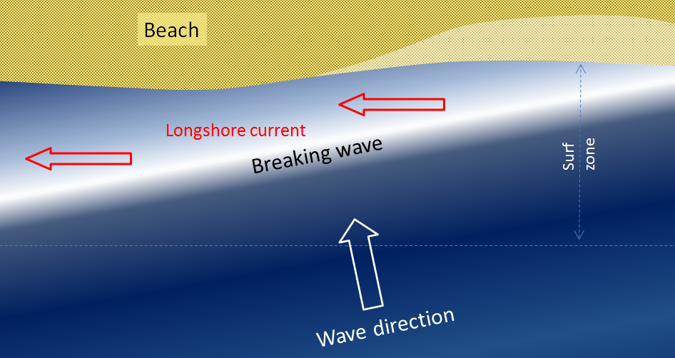
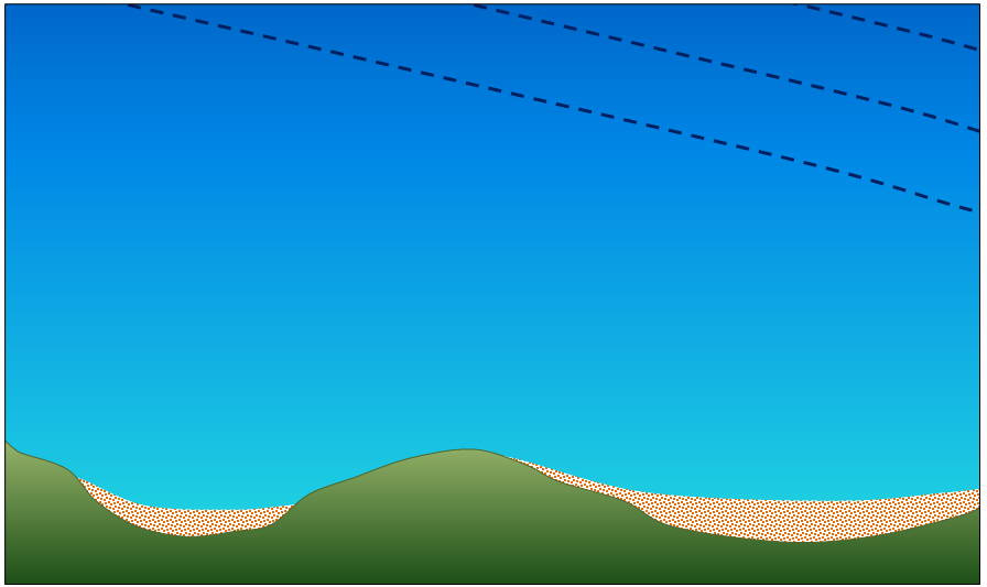
![Figure 17.8 The movement of particles on a beach as a result of swash and backwash [SE]](http://opentextbc.ca/geology/wp-content/uploads/sites/110/2015/08/swash-and-backwash.png)
![Figure 17.9 The formation of rip currents on a beach with strong surf [SE]](http://opentextbc.ca/geology/wp-content/uploads/sites/110/2015/08/rip-currents-on-a-beach-with-strong-surf.png)
![Figure 17.10 Rip currents on Tunquen Beach in central Chile [From NOAA http://www.ripcurrents.noaa.gov/images/Tunquen_Chile.jpg]](http://opentextbc.ca/geology/wp-content/uploads/sites/110/2015/08/Rip-currents-on-Tunquen-Beach.png)
![Figure 17.11 The approach of waves (white lines) in the Cox Bay area of Long Beach, Vancouver Island. The red arrows represent wave energy; most of that energy is focused on the headlands of Frank Island and Cox Point. [SE]](https://opentextbc.ca/physicalgeologyearle/wp-content/uploads/sites/145/2016/03/cox-2.png)
![Figure 17.12 A wave-cut platform in bedded sedimentary rock on Gabriola Island, B.C. The wave-eroded surface is submerged at high tide. [SE]](http://opentextbc.ca/geology/wp-content/uploads/sites/110/2015/08/A-wave-cut-platform.jpg)
![Figure 17.13 A stack on the Juan de Fuca Trail section of the southwestern shore of Vancouver Island. The rock surrounding the stack is part of a wave-cut platform. [SE]](http://opentextbc.ca/geology/wp-content/uploads/sites/110/2015/08/stack-on-the-Juan-de-Fuca-Trail.jpg)
![Figure 17.14 Top: An arch in tilted sedimentary rock at the mouth of the Barachois River, Newfoundland, July 2012. Bottom: The same location in June 2013. The arch has collapsed and a small stack remains. [Photo: Dr. David Murphy, used with permission]](https://opentextbc.ca/physicalgeologyearle/wp-content/uploads/sites/145/2016/03/barachois-2.png)
![Figure 17.15 Evolution of a straightened coast through the erosion to stacks and arches, sea cliffs, and wave-cut platforms [SE]](https://opentextbc.ca/physicalgeologyearle/wp-content/uploads/sites/145/2016/03/straightening-2.png)
![Figure 17.16 The components of a sandy marine beach [SE]](http://opentextbc.ca/geology/wp-content/uploads/sites/110/2015/08/components-of-a-sandy-marine-beach.png)
![Figure 17.17 The differences between summer and winter on beaches in areas where the winter conditions are rougher and waves have a shorter wavelength but higher energy. In winter, sand from the beach is stored offshore. [SE]](http://opentextbc.ca/geology/wp-content/uploads/sites/110/2015/08/differences-between-summer-and-winter-on-beaches.png)
![Figure 17.18 The formation of Goose Spit at Comox on Vancouver Island. The sand that makes up Goose Spit is derived from the erosion of Pleistocene Quadra Sand (a thick glaciofluvial sand deposit, as illustrated in the photo on the right). [SE]](https://opentextbc.ca/physicalgeologyearle/wp-content/uploads/sites/145/2016/03/comox-2.png)
![Figure 17.19 The Quadra Sand cliff at Comox, and the extensive concrete and rip-rap barrier that has been constructed to reduce erosion. Note that the waves (dashed lines) are approaching the shore at an angle, contributing to the longshore current. [SE]](http://opentextbc.ca/geology/wp-content/uploads/sites/110/2015/08/The-Quadra-Sand-cliff.png)
![Figure 17.20 A depiction of a baymouth bar and a tombolo [SE]](http://opentextbc.ca/geology/wp-content/uploads/sites/110/2015/08/baymouth-bar-and-a-tombolo.png)
![Figure 17.21 The process of formation of a tombolo in a wave shadow behind a nearshore island [SE]](http://opentextbc.ca/geology/wp-content/uploads/sites/110/2015/08/formation-of-a-tombolo-in-a-wave-shadow.png)
![Figure 17.22 A stack (with a wave-cut platform) connected to the mainland by a tombolo, Leboeuf Bay, Gabriola Island, B.C. [SE]](http://opentextbc.ca/geology/wp-content/uploads/sites/110/2015/08/A-stack-connected-to-the-mainland-by-a-tombolo.jpg)
![Figure 17.23 Assateague Island on the Maryland coast, U.S.A. This barrier island is about 60 km long and only 1 km to 2 km wide. The open Atlantic Ocean is to the right and the lagoon is to the left. This part of Assateague Island has recently been eroded by a tropical storm, which pushed massive amounts of sand into the lagoon. [http://soundwaves.usgs.gov/2014/04/images/DelmarvaAssateague_aerial_ViewCV.jpg]](http://opentextbc.ca/geology/wp-content/uploads/sites/110/2015/08/Assateague-Island-on-the-Maryland-coast.jpg)
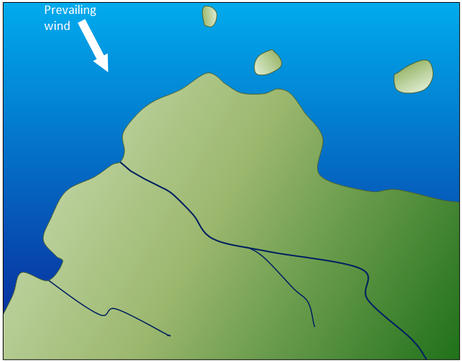
![Figure 17.24 Cross-section through a typical barrier or fringing reef [SE]](http://opentextbc.ca/geology/wp-content/uploads/sites/110/2015/08/Cross-section-through-a-typical-barrier-or-fringing-reef.png)
![Figure 17.25 Eustatic sea-level curve for the past 24 ka (sea-level rise resulting from the melting of glacial ice). Sea-level rise is global; the locations listed in the caption are the places where data were acquired to create this diagram. [https://en.wikipedia.org/wiki/Sea_level_rise#/media/File:Post-Glacial_Sea_Level.png]](http://opentextbc.ca/geology/wp-content/uploads/sites/110/2015/08/Eustatic-sea-level-curve-for-the-past-24-ka.png)
![Figure 17.26 This stream is on the southwest coast of Vancouver Island near Sooke. Like many other streams along this coast, it used to flow directly into the ocean, but the land has been uplifted by post-glacial isostatic rebound. [SE]](http://opentextbc.ca/geology/wp-content/uploads/sites/110/2015/08/uplifted-by-post-glacial-isostatic-rebound.jpg)
![Figure 17.27 Howe Sound, north of Vancouver, is a fiord with well-defined glacial erosion features. [SE]](http://opentextbc.ca/geology/wp-content/uploads/sites/110/2015/08/Howe-Sound.jpg)
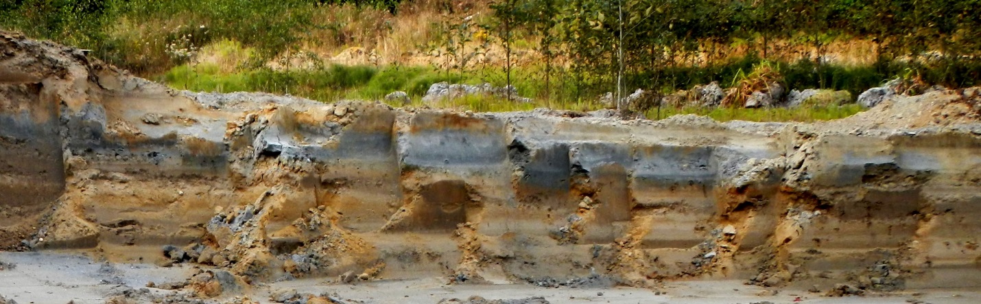
![Figure 17.28 The seawall at Stanley Park, Vancouver [https://commons.wikimedia.org/wiki/File:Seawall2.jpg]](https://opentextbc.ca/physicalgeologyearle/wp-content/uploads/sites/145/2016/03/stanley-2.png)
![Figure 17.29 Map of the impact of breakwaters (or groynes) on beach formation at Sunset Beach, Vancouver [SE]](http://opentextbc.ca/geology/wp-content/uploads/sites/110/2015/08/Map-of-the-impact-of-breakwaters-.png)
![Figure 17.30 Photograph of the impact of breakwaters on beach development at Sunset Beach, Vancouver [by Isaac Earle, used with permission]](http://opentextbc.ca/geology/wp-content/uploads/sites/110/2015/08/impact-of-breakwaters-on-beach-development-at-Sunset-Beach.jpg)
![Figure 17.31 A groyne at Crescent Beach, Surrey, B.C. [https://commons.wikimedia.org/wiki/File:Cresbeach-groyne.jpg]](http://opentextbc.ca/geology/wp-content/uploads/sites/110/2015/08/groyne-at-Crescent-Beach.jpg)
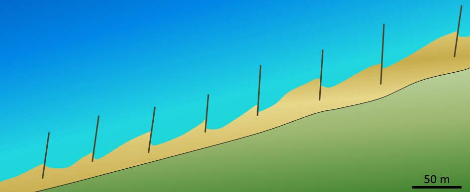


![Figure 18.1 Oceanic crust (pillow basalt) from the Paleogene Metchosin Igneous Complex, near Sooke, on Vancouver Island. The view is about 1.5 m across. [SE]](http://opentextbc.ca/geology/wp-content/uploads/sites/110/2015/08/Oceanic-crust-from-the-Paleogene-Metchosin-Igneous-Complex.jpg)
![Figure 18.2 The topography of the Atlantic Ocean sea floor between 0° and 50° north. Red and yellow colours indicate less than 2,000 m depth; green less than 3,000 m; blue 4,000 m to 5,000 m; and purple greater than 6,000 m. [from NASA/CNES at: http://topex.ucsd.edu/marine_topo/jpg_images/topo8.jpg]](http://opentextbc.ca/geology/wp-content/uploads/sites/110/2015/08/The-topography-of-the-Atlantic-Ocean-sea-floor.jpg)
![Figure 18.3 The generalized topography of the Pacific Ocean sea floor between Japan and British Columbia. The vertical exaggeration is approximately 200 times. [SE]](http://opentextbc.ca/geology/wp-content/uploads/sites/110/2015/08/generalized-topography-of-the-Pacific-Ocean-sea-floor.png)
![Figure 18.4 The generalized topography of the Atlantic Ocean floor within 300 km of Nova Scotia. The vertical exaggeration is approximately 25 times. The panel at the bottom shows the same profile without vertical exaggeration. [SE]](http://opentextbc.ca/geology/wp-content/uploads/sites/110/2015/08/Atlantic-Ocean-floor-within-300-km-of-Nova-Scotia.png)
![Figure 18.5 The generalized topography of the Pacific Ocean floor in the area of the Marianas Trench, near Guam. The dashed grey line represents the subduction of the Pacific Plate (to the right) beneath the Philippine Plate (to the left). [SE]](http://opentextbc.ca/geology/wp-content/uploads/sites/110/2015/08/Pacific-Ocean-floor-in-the-area-of-the-Marianas-Trench.png)
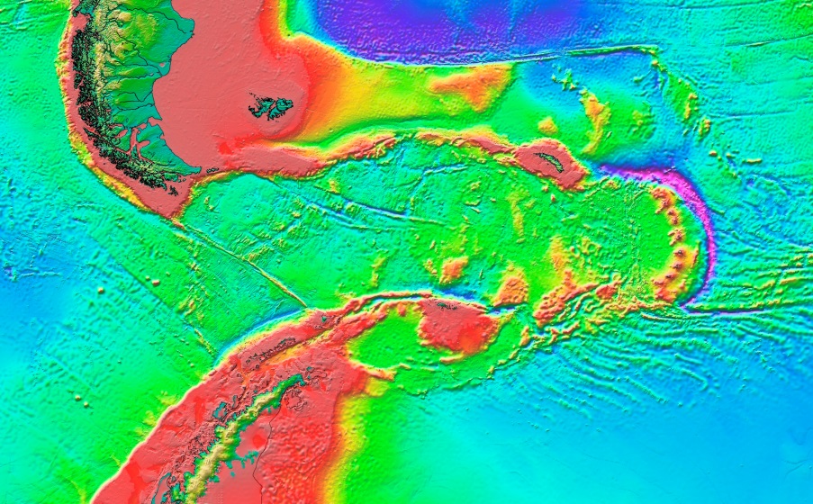
![Figure 18.6 Schematic representation of the lithologic layers of typical oceanic crust [SE]](http://opentextbc.ca/geology/wp-content/uploads/sites/110/2015/08/Schematic-representation-of-the-lithologic-layers.png)
![Figure 18.7 The age of the oceanic crust [SE after NOAA at http://www.ngdc.noaa.gov/mgg/ocean_age/data/2008/image/age_oceanic_lith.jpg]](http://opentextbc.ca/geology/wp-content/uploads/sites/110/2015/08/The-age-of-the-oceanic-crust.png)
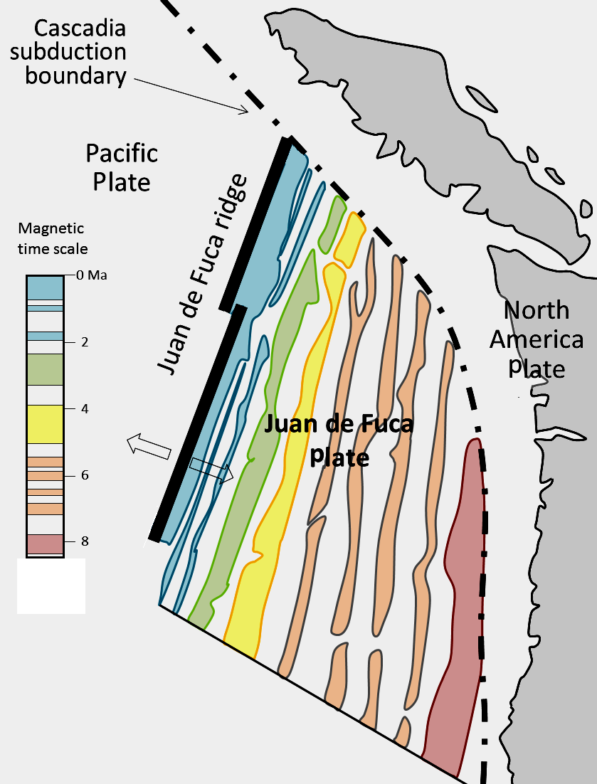
![Figure 18.8 The formation of a fringing reef, a barrier reef, and an atoll around a subsiding tropical volcanic island. [SE]](http://opentextbc.ca/geology/wp-content/uploads/sites/110/2015/08/fringing-reef-a-barrier-reef-and-an-atoll.png)
![Figure 18.9 The distribution of sediment types on the sea floor. Within each coloured area, the type of material shown is what dominates, although other materials are also likely to be present. [SE]](http://opentextbc.ca/geology/wp-content/uploads/sites/110/2015/08/distribution-of-sediment-types-on-the-sea-floor.png)
![Figure 18.10 Foraminifera from the Ambergris Caye area of Belize. Most of the shells are about 1 mm across. [SE]](http://opentextbc.ca/geology/wp-content/uploads/sites/110/2015/08/Ambergris-Caye-area-of-Belize.jpg)
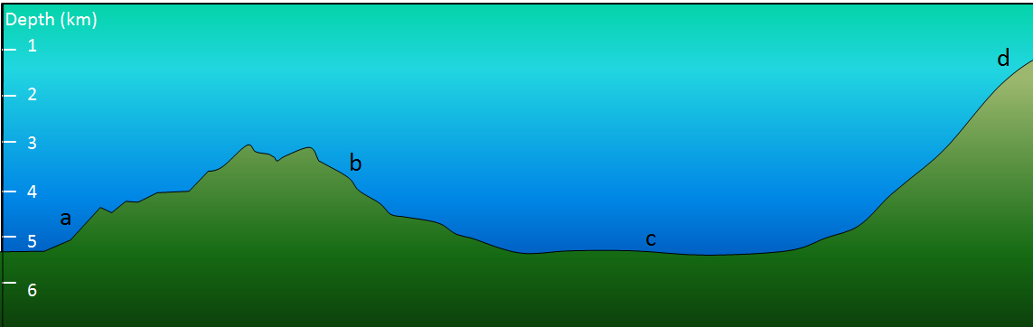
![Figure 18.11 Left: Methane hydrate within muddy sea-floor sediment from an area offshore from Oregon. [https://upload.wikimedia.org/wikipedia/commons/4/49/Gashydrat_im_Sediment.JPG] Right: Methane hydrate on fire [http://www.usgs.gov/blogs/features/files/2012/01/New-Image.jpg]](https://opentextbc.ca/physicalgeologyearle/wp-content/uploads/sites/145/2016/03/methane-hydrate-2.png)
![Figure 18.12 The proportions (by weight) of the major dissolved elements in ocean water [SE]](http://opentextbc.ca/geology/wp-content/uploads/sites/110/2015/08/proportions-of-the-major-dissolved-elements-in-ocean-water.png)
![Figure 18.13 The distribution of salinity in Earth’s oceans and major seas [https://upload.wikimedia.org/wikipedia/commons/d/d5/WOA09_sea-surf_SAL_AYool.png]](http://opentextbc.ca/geology/wp-content/uploads/sites/110/2015/08/distribution-of-salinity-in-Earth’s-oceans.png)
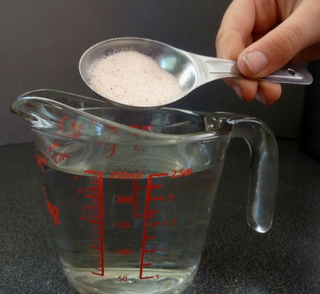
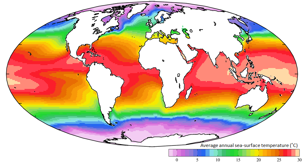
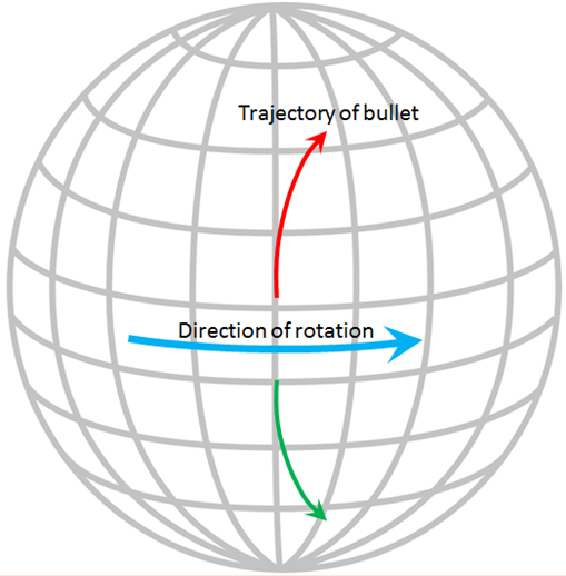
![Figure 18.15 Overview of the main open-ocean currents. Red arrows represent warm water moving toward colder regions. Blue arrows represent cold water moving toward warmer regions. Black arrows represent currents that don’t involve significant temperature changes. [From: https://upload.wikimedia.org/wikipedia/commons/9/9b/Corrientes-oceanicas.png]](http://opentextbc.ca/geology/wp-content/uploads/sites/110/2015/08/the-main-open-ocean-currents.png)
![Figure 18.16 An iceberg floating past Exploits Island, on the Newfoundland Current [https://commons.wikimedia.org/wiki/File:Newfoundland_Iceberg_just_off_Exploits_Island.jpg]](http://opentextbc.ca/geology/wp-content/uploads/sites/110/2015/08/iceberg-floating-past-Exploits-Island.jpg)
![Figure 18.17 A depiction of the vertical movement of water along a north-south cross-section through the Atlantic basin [SE]](http://opentextbc.ca/geology/wp-content/uploads/sites/110/2015/08/vertical-movement-of-water-along-a-north-south-cross-section.png)
![Figure 18.18 The thermohaline circulation system, also known as the Global Ocean Conveyor [from NASA at: https://en.wikipedia.org/wiki/Thermohaline_circulation#/media/File:Thermohaline_Circulation_2.png]](http://opentextbc.ca/geology/wp-content/uploads/sites/110/2015/08/thermohaline-circulation-system.png)
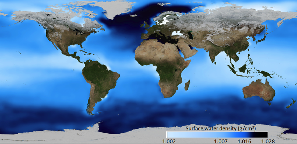
![Figure 19.1 Core from Ocean Drilling Program hole 1220b (southeast of Hawaii) showing the boundary between the Paleocene and the Eocene (at 55.8 Ma). Marine life was decimated during the 100,000 years of the Paleocene-Eocene thermal maximum, and the dark part of the core represents the absence of carbonate sediment from planktonic organisms. The scale is in centimetres. [SE, after Ocean Drilling Program, used with permission]](http://opentextbc.ca/geology/wp-content/uploads/sites/110/2015/08/Core-from-Ocean-Drilling-Program-hole.png)
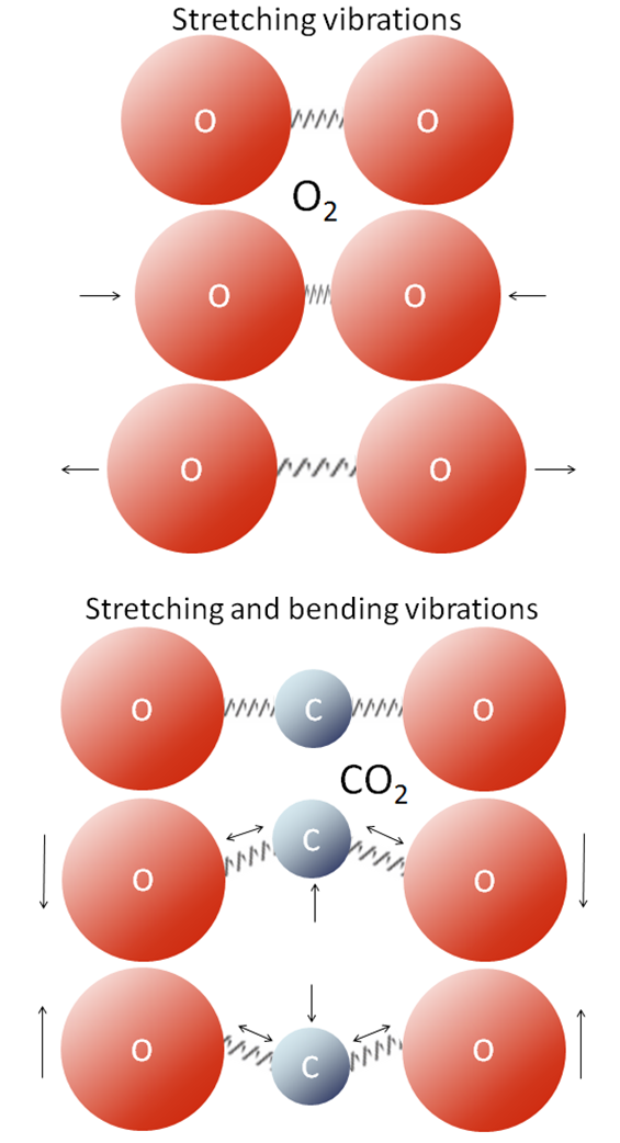
![Figure 19.2 The life cycle of our Sun and of other similar stars [from https://upload.wikimedia.org/wikipedia/commons/thumb/5/55/Solar_Life_Cycle.svg/2000px-Solar_Life_Cycle.svg.png]](http://opentextbc.ca/geology/wp-content/uploads/sites/110/2015/08/life-cycle-of-our-Sun.png)
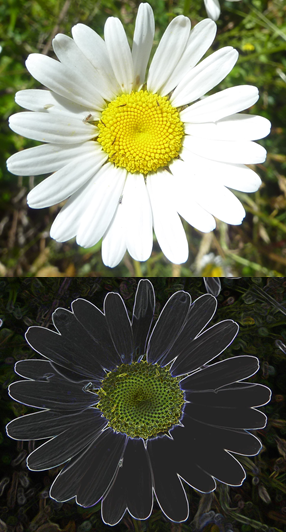
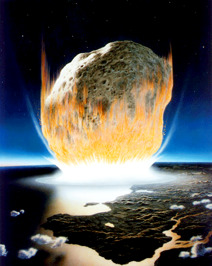
![Figure 19.3 The cycles of Earth’s orbit and rotation [a: SE after https://upload.wikimedia.org/wikipedia/commons/thumb/d/da/Eccentricity_zero.svg/1163px-Eccentricity_zero.svg.png], b: https://upload.wikimedia.org/wikipedia/commons/thumb/a/ae/Earth_obliquity_range.svg/2000px-Earth_obliquity_range.svg.png] c: https://upload.wikimedia.org/wikipedia/commons/thumb/4/43/ Earth_precession.svg/2000px-Earth_precession.svg.png]](https://opentextbc.ca/physicalgeologyearle/wp-content/uploads/sites/145/2016/03/milankovitch.png)
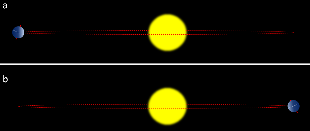
![Figure 19.5 Insolation at 65° N in July compared with Antarctic ice core temperatures [By SE, using data from Valerie Masson-Delmotte, EPICA Dome C ice core 800KYr deuterium data and temperature estimates WDCA Contribution Series Number : 2007 -091 NOAA/NCDC Paleoclimatology Program, Boulder CO, USA. Retrieved from: ftp://ftp.ncdc.noaa.gov/pub/data/paleo/icecore/antarctica/epica_domec/edc3deuttemp2007.txt and from Berger, A. and Loutre, M.F. (1991). Insolation values for the climate of the last 10 million years. Quaternary Science Reviews, 10, 297-317.]](http://opentextbc.ca/geology/wp-content/uploads/sites/110/2015/08/Insolation-at-65N-in-July.png)
![Figure 19.6 Variations in the ENSO index from 1950 to mid-2016 [SE after NOAA at: http://www.esrl.noaa.gov/psd/enso/mei/]](https://opentextbc.ca/physicalgeologyearle/wp-content/uploads/sites/145/2016/03/enso-2016.png)
![Figure 19.7 Typical albedo values for Earth surfaces [SE]](http://opentextbc.ca/geology/wp-content/uploads/sites/110/2015/08/Typical-albedo-values-for-Earth-surfaces.png)
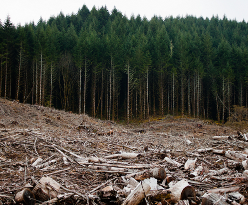
![Figure 19.8 A degrading permafrost site on the north coast of Alaska [http://alaska.usgs.gov/science/interdisciplinary_science/cae/images/theme2_fig2_lg.jpg]](http://opentextbc.ca/geology/wp-content/uploads/sites/110/2015/08/degrading-permafrost-site.jpg)
![Figure 19.9 World population growth over the past 12,000 years [by SE from data at: http://ourworldindata.org/roser/graphs/WorldPopulationAnnual12000years_interpolated_HYDEandUN/WorldPopulationAnnual12000years_interpolated_HYDEandUN.csv]](http://opentextbc.ca/geology/wp-content/uploads/sites/110/2015/08/World-population-growth-over-the-past-12000-years-.png)
![Figure 19.10 Global mean annual temperatures for the period from 1880 to 2015 [by SE from data at NASA at: http://data.giss.nasa.gov/gistemp/tabledata_v3/GLB.Ts+dSST.txt]](https://opentextbc.ca/physicalgeologyearle/wp-content/uploads/sites/145/2016/03/giss-ls-2015.png)
![Figure 19.11 The relative importance of factors that are contributing to anthropogenic warming [from http://www.ipcc.ch/report/graphics/index.php?t=Assessment%20Reports&r=AR5%20-%20WG1&f=SPM]](http://opentextbc.ca/geology/wp-content/uploads/sites/110/2015/08/importance-of-factors-that-are-contributing-to-anthropogenic-warming.jpg)
![Figure 19.12 Projected global temperature increases for the 21st century based on a range of different IPCC scenarios of future political and technological variables [from https://www.ipcc.ch/publications_and_data/ar4/wg1/en/fig/figure-spm-5-l.png]](https://opentextbc.ca/physicalgeologyearle/wp-content/uploads/sites/145/2016/03/scenarios-2.png)
![Figure 19.13 Projected sea-level increases to 2100, showing likely range (grey) and possible maximum [Adapted by SE from: http://nca2014.globalchange.gov/report/our-changing-climate/sea-level-rise#intro-section-2 based on data in Parris et al., 2012, NOAA]](http://opentextbc.ca/geology/wp-content/uploads/sites/110/2015/08/Projected-sea-level-increases-to-2100.png)
![Figure 19.14 Damage to the Casino Pier, Seaside Heights, New Jersey, from Hurricane Sandy, November 2012 [https://upload.wikimedia.org/wikipedia/commons/c/cb/Hurricane_Sandy_New_Jersey_Pier.jpg]](http://opentextbc.ca/geology/wp-content/uploads/sites/110/2015/08/Damage-to-the-Casino-Pier.jpg)
![Figure 19.15 Relationship between Atlantic tropical storm cumulative annual intensity and Atlantic sea-surface temperatures [By SE from data at: http://wind.mit.edu/~emanuel/Papers_data_graphics.htm]](http://opentextbc.ca/geology/wp-content/uploads/sites/110/2015/08/Relationship-between-Atlantic-tropical-storm-cumulative-annual-intensity-and-Atlantic-sea-surface-temperatures.png)
![Figure 19.16 Global precipitation anomalies compared with the average over the period from 1901 to 2000 [By NASA, from: http://www.epa.gov/climatechange/science/indicators/weather-climate/precipitation.html]](https://opentextbc.ca/physicalgeologyearle/wp-content/uploads/sites/145/2016/03/precipitation-2.png)
![Figure 19.17 Change in precipitation amounts over the period 1945 to 2005 for 29 stations in British Columbia [By SE, using data from Environment Canada]](http://opentextbc.ca/geology/wp-content/uploads/sites/110/2015/08/Change-in-precipitation-amounts-over-the-period-1945-to-2005.png)
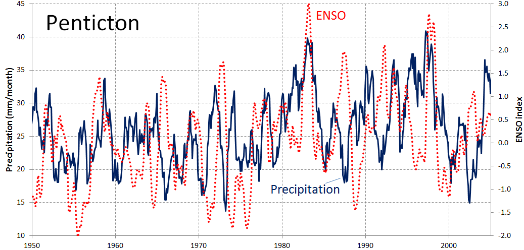
![Figure 19.18 Mountain pine beetle damage in Manning Park, British Columbia [https://upload.wikimedia.org/wikipedia/en/7/7c/Pine_Beetle_in_Manning_Park.jpg]](http://opentextbc.ca/geology/wp-content/uploads/sites/110/2015/08/Mountain-pine-beetle-damage.jpg)
![Figure 19.19 Numbers of various types of disasters between 1971 and 2010 [From WMO atlas of mortality and economic Losses from weather, climate and water extremes, 2014]](http://opentextbc.ca/geology/wp-content/uploads/sites/110/2015/08/Numbers-of-various-types-of-disasters-between-1971-and-2010.png)
![Figure 19.20 Temperature anomalies across Russia and neighbouring regions during July 2010 [http://earthobservatory.nasa.gov/IOTD/view.php?id=45069]](http://opentextbc.ca/geology/wp-content/uploads/sites/110/2015/08/Temperature-anomalies-across-Russia.png)
![Figure 20.1 The open pit (background) and waste-rock piles (middle) of the Highland Valley Copper Mine at Logan Lake, British Columbia [Photo by Russell Hartlaub, used with permission]](http://opentextbc.ca/geology/wp-content/uploads/sites/110/2015/08/Highland-Valley-Copper-Mine-at-Logan-Lake.jpg)
![Figure 20.2 The main components of a tablet computer [SE, base photograph from https://upload.wikimedia.org/wikipedia/commons/8/8d/IPad_Air.png]](http://opentextbc.ca/geology/wp-content/uploads/sites/110/2015/08/main-components-of-a-tablet-computer.png)
![[https://upload.wikimedia.org/wikipedia/commons/f/fd/Ballpoint-pen-parts.jpg]](https://opentextbc.ca/physicalgeologyearle/wp-content/uploads/sites/145/2016/06/ball-point-2.png)
![Figure 20.3 The value of various Canadian mining sectors in 2013 [SE from data at http://www.nrcan.gc.ca/mining-materials/publications/8772]](http://opentextbc.ca/geology/wp-content/uploads/sites/110/2015/08/value-of-various-Canadian-mining-sectors-in-2013.png)
![Figure 20.4 The nickel smelter at Thompson, Manitoba [https://en.wikipedia.org/wiki/Thompson,_Manitoba#/media/File:Vale_Nickel_Mine.JPG]](http://opentextbc.ca/geology/wp-content/uploads/sites/110/2015/08/nickel-smelter-at-Thompson.jpg)
![Figure 20.5 Left: A black smoker on the Juan de Fuca Ridge off the west coast of Vancouver Island. Right: A model of the formation of a volcanogenic massive sulphide deposit on the sea floor. [left: NOAA at: http://oceanexplorer.noaa.gov/okeanos/explorations/10index/background/plumes/media/black_smoker.html, right: SE]](https://opentextbc.ca/physicalgeologyearle/wp-content/uploads/sites/145/2016/06/black-smoker-2.png)
![Figure 20.6 A model for the formation of a porphyry deposit around an upper-crustal porphyritic stock and associated vein deposits. [SE]](http://opentextbc.ca/geology/wp-content/uploads/sites/110/2015/08/the-formation-of-a-porphyry-deposit.png)
![Figure 20.7 Banded iron formation from an unknown location in North America on display at a museum in Germany. The rock is about 2 m across. The dark grey layers are magnetite and the red layers are hematite. Chert is also present. [https://upload.wikimedia.org/wikipedia/commons/5/5f/Black-band_ironstone_%28aka%29.jpg]](http://opentextbc.ca/geology/wp-content/uploads/sites/110/2015/08/Banded-iron-formation.jpg)
![Figure 20.8 Model of the formation of unconformity-type uranium deposits of the Athabasca Basin, Saskatchewan [SE]](https://opentextbc.ca/physicalgeologyearle/wp-content/uploads/sites/145/2016/06/athabasca-3.png)
![Figure 20.9 Underground at the Myra Falls Mine, Vancouver Island. [SE]](http://opentextbc.ca/geology/wp-content/uploads/sites/110/2015/08/Underground-at-the-Myra-Falls-Mine.jpg)
![Figure 20.10 Schematic cross-section of a typical underground mine. [SE]](http://opentextbc.ca/geology/wp-content/uploads/sites/110/2015/08/Schematic-cross-section-of-a-typical-underground-mine.png)
![Figure 20.11 Entrance to an exploratory decline (white arrow) for the New Afton Mine situated in the side of the open pit of the old Afton Mine, near Kamloops, B.C. [SE]](http://opentextbc.ca/geology/wp-content/uploads/sites/110/2015/08/Entrance-to-an-exploratory-decline.png)
![Figure 20.12 The tailings pond at the Myra Falls Mine on Vancouver Island. The dry rock in the middle of the image is waste rock. The structure on the right is the headframe for the mine shaft. Myra Creek flows between the tailings pond and the headframe. [SE]](http://opentextbc.ca/geology/wp-content/uploads/sites/110/2015/08/tailings-pond-at-the-Myra-Falls-Mine.jpg)
![Figure 20.13 The tailings pond (lower left) at Myra Falls Mine with settling ponds (right) for processing water from the concentrator. [SE]](http://opentextbc.ca/geology/wp-content/uploads/sites/110/2015/08/The-tailings-pond-at-Myra-Falls-Mine-with-settling-ponds.jpg)
![Figure 20.14a The Mt. Polley Mine area prior to the dam breach of August 2014. The tailings were stored in the area labelled “retention basin.” [https://en.wikipedia.org/wiki/Mount_Polley_mine_disaster]](http://opentextbc.ca/geology/wp-content/uploads/sites/110/2015/08/The-Mt.-Polley-Mine-area-prior-to-the-dam-breach.jpg)
![Figure 20.14b The Mt. Polley Mine area after the tailings dam breach of August 2014. The water and tailings released flowed into Hazeltine Creek, and Polley and Quesnel Lakes. [https://en.wikipedia.org/wiki/Mount_Polley_mine_disaster]](http://opentextbc.ca/geology/wp-content/uploads/sites/110/2015/08/Mt.-Polley-Mine-area-after-the-tailings-dam-breach.jpg)
![Figure 20.15 Sand and gravel in an aggregate pit near Nanaimo, BC. [SE]](http://opentextbc.ca/geology/wp-content/uploads/sites/110/2015/08/Sand-and-gravel-in-an-aggregate-pit.jpg)
![Figure 20.16 Triassic Quatsino Formation limestone being quarried on Texada Island, B.C. [SE]](http://opentextbc.ca/geology/wp-content/uploads/sites/110/2015/08/Triassic-Quatsino-Formation-limestone.jpg)
![Figure 20.17 Slate used as a facing material on a concrete building column in Vancouver [SE]](http://opentextbc.ca/geology/wp-content/uploads/sites/110/2015/08/Slate-used-as-a-facing-material.jpg)
![Figure 20.18 Formation of coal: (a) accumulation of organic matter within a swampy area; (b) the organic matter is covered and compressed by deposition of a new layer of clastic sediments; (c) with greater burial, lignite coal forms; and (d) at even greater depths, bituminous and eventually anthracite coal form. [SE]](https://opentextbc.ca/physicalgeologyearle/wp-content/uploads/sites/145/2016/06/coal-2.png)
![Figure 20.19 The Highvale Mine (background) and the Sundance (right) and Keephills (left) generating stations on the southern shore of Wabamun Lake, Alberta [SE]](http://opentextbc.ca/geology/wp-content/uploads/sites/110/2015/08/Highvale-Mine-and-the-Sundance.jpg)
![Figure 20.20 The depth and temperature limits for biogenic gas, oil, and thermogenic gas [SE]](http://opentextbc.ca/geology/wp-content/uploads/sites/110/2015/08/depth-and-temperature-limits-for-biogenic-gas.png)
![Figure 20.21 Migration of oil and gas from source rocks into traps in reservoir rocks [SE]](http://opentextbc.ca/geology/wp-content/uploads/sites/110/2015/08/Migration-of-oil-and-gas.png)
![Figure 20.22 Seismic section through the East Breaks Field in the Gulf of Mexico. The dashed red line marks the approximate boundary between deformed rocks and younger undeformed rocks. The wiggly arrows are interpreted migration paths. The total thickness of this section is approximately 5 km. [SE after http://wiki.aapg.org/File:Sedimentary-basin-analysis_fig4-55.png]](http://opentextbc.ca/geology/wp-content/uploads/sites/110/2015/08/Seismic-section-through-the-East-Breaks-Field.png)
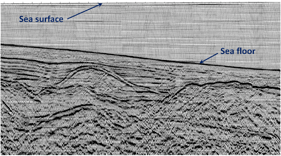
![Figure 20.23 Schematic cross-section of northern Alberta showing the source rocks and location of the Athabasca Oil Sands [SE]](http://opentextbc.ca/geology/wp-content/uploads/sites/110/2015/08/Schematic-cross-section-of-northern-Alberta.png)
![Figure 20.24 Depiction of the process of directional drilling and fracking to recover gas from impermeable rocks. The light blue arrows represent the potential for release of fracking chemicals to aquifers. [by SE, after https://en.wikipedia.org/wiki/Hydraulic_fracturing#/media/File:HydroFrac2.svg]](http://opentextbc.ca/geology/wp-content/uploads/sites/110/2015/08/Depiction-of-the-process-of-directional-drilling-and-fracking.png)
![Figure 20.25 Diamond mines in the Lac de Gras region, Nunavut. The twin pits of the Diavik Mine are visible in the lower right on an island within Lac de Gras. The five pits of the Ekati mine are also visible, on the left and the upper right. The two main mine centres are 25 km apart. [http://earthobservatory.nasa.gov/IOTD/view.php?id=84085&src=eoa-iotd]](http://opentextbc.ca/geology/wp-content/uploads/sites/110/2015/08/Diamond-mines-in-the-Lac-de-Gras-region.jpg)

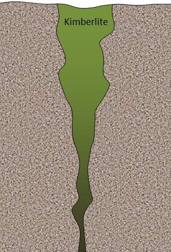
![Figure 21.1 Crowsnest Mountain in the southern Alberta Rockies is made up of Paleozoic rocks that were uplifted by continental convergence during the Mesozoic, and then eroded by glaciation during the Cenozoic [SE]](http://opentextbc.ca/geology/wp-content/uploads/sites/110/2015/08/Crowsnest-Mountain.jpg)
![Figure 21.2 The path of Laurentia over the past 650 Ma [SE]](http://opentextbc.ca/geology/wp-content/uploads/sites/110/2015/08/The-path-of-Laurentia.png)
![Figure 21.3 The main provinces of Laurentia. The pink areas are the oldest; light yellow are the youngest. All of the areas south and west of the dotted red line are now covered with younger rocks. The white areas represent rocks that were added to North America since 700 Ma. [SE]](http://opentextbc.ca/geology/wp-content/uploads/sites/110/2015/08/main-provinces-of-Laurentia.png)
![Figure 21.4 Geological map of Canada from the Geological Survey of Canada [http://geoscan.nrcan.gc.ca/starweb/geoscan/servlet.starweb?path=geoscan/fulle.web&search1=R=208175]](http://opentextbc.ca/geology/wp-content/uploads/sites/110/2015/08/Geological-map-of-Canada.png)
![Figure 21.5 Geological features of the Canadian Shield of western Canada. A.B.: Athabasca Basin, T.B.: Thelon Basin, and TMZ: Taltson Magmatic Zone [ By SE after: http://geoscan.nrcan.gc.ca/starweb/geoscan/servlet.starweb?path=geoscan/fulle.web&search1=R=208175]](http://opentextbc.ca/geology/wp-content/uploads/sites/110/2015/08/Canadian-Shield-of-western-Canada.png)
![Figure 21.6 A sample of the Acasta Gneiss on display at the Natural History Museum in Vienna [https://commons.wikimedia.org/wiki/File:Acasta_gneiss.jpg]](http://opentextbc.ca/geology/wp-content/uploads/sites/110/2015/08/Acasta-Gneiss.jpg)
![Figure 21.7 Precambrian rocks in southern B.C. and Alberta [ By SE after: http://geoscan.nrcan.gc.ca/starweb/geoscan/servlet.starweb?path=geoscan/fulle.web&search1=R=208175]](http://opentextbc.ca/geology/wp-content/uploads/sites/110/2015/08/Precambrian_rocks_in_southern-BC.png)
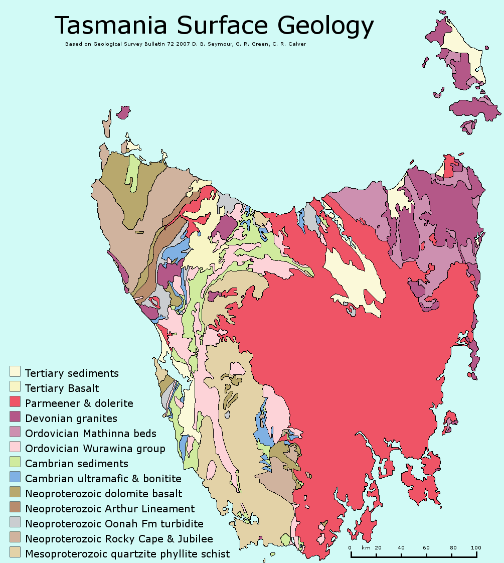
![Figure 21.8 Late Proterozoic Toby Formation mudstone with glacial dropstones south of Cranbrook, B.C. [SE]](https://opentextbc.ca/physicalgeologyearle/wp-content/uploads/sites/145/2016/03/toby-a.png)
![Figure 21.9 The Cambrian Burgess Shale at the Walcott Quarry, Yoho Park, B.C., with Wapta Mountain in the upper right. [SE]](http://opentextbc.ca/geology/wp-content/uploads/sites/110/2015/08/Cambrian-Burgess-Shale-at-the-Walcott-Quarry.jpg)
![Figure 21.10 The Paleozoic sedimentary rocks of southern Manitoba along a section extending from the Saskatchewan border on the left to the Winnipeg area on the right. The section is 400 km wide and 1,800 m high, and the vertical exaggeration is about 100 times. The dip of the beds is also exaggerated by 100 times; their original and current attitudes are close to horizontal. [SE]](http://opentextbc.ca/geology/wp-content/uploads/sites/110/2015/08/Paleozoic-sedimentary-rocks.png)
![Figure 21.11 The distribution of continents in the early Carboniferous, showing the terranes that later became attached to the west coast of North America. The light blue areas are continental shelves, the white is ice of the Karoo Glaciation, and the red line shows subduction of oceanic crust beneath Laurentia. Panthalassic is the name for the huge ocean that preceded the Pacific Ocean. [SE based on information from Christopher Scotese at http://www.scotese.com/]](http://opentextbc.ca/geology/wp-content/uploads/sites/110/2015/08/continents-in-the-early-Carboniferous.png)
![Figure 21.12 The Carboniferous Mt. Mark Formation on Vancouver Island is part of the Wrangellia Terrane, which arrived on the edge of North America during the Cretaceous. [SE]](http://opentextbc.ca/geology/wp-content/uploads/sites/110/2015/08/Carboniferous-Mt-Mark-Formation.jpg)
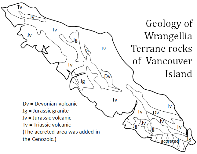
![Figure 21.13 Model of the accretion of the Intermontane and Insular Superterranes to the west coast of North America during the Mesozoic. Subduction zones are the red-toothed lines. The brown triangles represent volcanoes. [SE]](http://opentextbc.ca/geology/wp-content/uploads/sites/110/2015/08/Intermontane-and-Insular-Superterranes.png)
![Figure 21.14 A generalized overview of the accreted terranes of B.C., Yukon, and Alaska. The Intermontane terranes are in green, the Insular terranes in purple, and the Outboard terranes in yellow. The Coast Plutonic Complex (CPC) formed in situ and is not a terrane. [SE after Yukon and BC Geological Surveys]](http://opentextbc.ca/geology/wp-content/uploads/sites/110/2015/08/the-accreted-terranes-of-BC.png)
![Figure 21.15 Cross-section of the accretion of the Intermontane Superterrane to the west coast of North America and the resulting compression, folding, and thrusting of North American sedimentary rocks. In the Late Cretaceous, it was the accretion of the Insular Superterrane, pushing against the Intermontane Superterrane, that did most of the work. [SE]](http://opentextbc.ca/geology/wp-content/uploads/sites/110/2015/08/accretion-of-the-Intermontane-Superterrane.png)
![Figure 21.16 Tight folds in sedimentary rocks of the Rocky Mountains near Field, B.C. [SE]](http://opentextbc.ca/geology/wp-content/uploads/sites/110/2015/08/Tight-folds-in-sedimentary-rocks-of-the-Rocky-Mountains.jpg)
![Figure 21.17 Folding of sedimentary rocks at Mt. Rae, Alberta. [https://upload.wikimedia.org/wikipedia/commons/e/e5/Mt-Rae-Alberta-Canada-aerial1.jpg]](http://opentextbc.ca/geology/wp-content/uploads/sites/110/2015/08/Folding-of-sedimentary-rocks.jpg)
![Figure 21.18 The McConnell Thrust at Mt. Yamnuska near Exshaw, Alberta. Carbonate rocks of Cambrian age have been thrust over top of Cretaceous mudstone. [SE]](http://opentextbc.ca/geology/wp-content/uploads/sites/110/2015/08/McConnell-Thrust-at-Mt-Yamnuska.png)
![Figure 21.19 The Lewis Thrust at Crowsnest Mountain near Frank, Alberta. Carbonate rocks of Devonian and Carboniferous age have been pushed 80 km to the east and thrust over top of Cretaceous mudstone. [SE]](http://opentextbc.ca/geology/wp-content/uploads/sites/110/2015/08/Lewis-Thrust-at-Crowsnest-Mountain.png)
![Figure 21.20 Jurassic (J) and Cretaceous (K) granitic bodies in south-central B.C. [SE]](http://opentextbc.ca/geology/wp-content/uploads/sites/110/2015/08/Jurassic-and-Cretaceous-granitic-bodies.png)
![Figure 21.21 Cretaceous granite at The Lions, north of Vancouver, with Howe Sound in the background [Isaac Earle, used with permission]](http://opentextbc.ca/geology/wp-content/uploads/sites/110/2015/08/Cretaceous-granite-at-The-Lions.jpg)
![Figure 21.22 The distribution of Mesozoic sedimentary rocks in the Western Canada Sedimentary Basin. J stands for Jurassic and Pc for Paleocene. The lines of the cross-sections of Figures 21.10 and 21.23 are shown. [SE after Alberta Geological Survey]](http://opentextbc.ca/geology/wp-content/uploads/sites/110/2015/08/distribution-of-Mesozoi-sedimentary-rocks.png)
![Figure 21.23 A cross-section showing the Mesozoic sedimentary rocks in the WCSB from the Rocky Mountain foothills to north-central Saskatchewan [SE after Alberta Geological Survey]](http://opentextbc.ca/geology/wp-content/uploads/sites/110/2015/08/Mesozoic-sedimentary-rocks-in-the-WCSB.png)
![Figure 21.24 The Horseshoe Canyon Formation near Drumheller, Alberta [SE]](http://opentextbc.ca/geology/wp-content/uploads/sites/110/2015/08/Horseshoe-Canyon-Formation.jpg)
![Figure 21.25 Depiction of some of the large herbivorous dinosaurs from the upper part of the Dinosaur Park Formation. Left to right: the ceratopsian Pentaceratops , the hadrosaur Lambeosaurus eating from a tall tree, the ceratopsian Styracosaurus, the ankylosuar Scolosaurus, the hadrosaur Prosaurolophus (in the distance), the ankylosaur Panoplosaurus, and a herd of Styracosaurs in the background. [by J.T. Csotonyi at https://upload.wikimedia.org/wikipedia/commons/e/e9/Dinosaur_park_formation_fauna.png]](http://opentextbc.ca/geology/wp-content/uploads/sites/110/2015/08/large-herbivorous-dinosaurs.png)
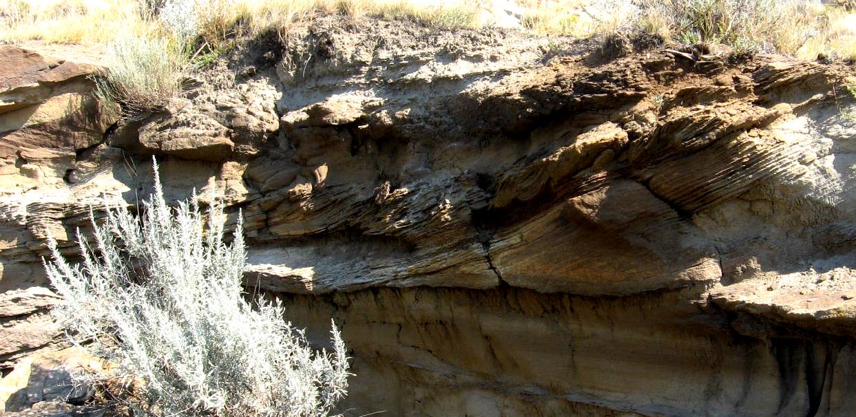
![Figure 21.26 East-west cross-section showing the accretion of the Pacific Rim and Crescent Terranes beneath Vancouver Island, and the ongoing subduction of the Juan de Fuca Plate. The dashed lines are inactive faults. [SE after Geological Survey of Canada]](http://opentextbc.ca/geology/wp-content/uploads/sites/110/2015/08/accretion-of-the-Pacific-Rim-and-Crescent-Terranes.png)
![Figure 21.27 The distribution of Pacific Rim and Crescent Terrane rocks on Vancouver Island [SE after Geological Survey of Canada]](http://opentextbc.ca/geology/wp-content/uploads/sites/110/2015/08/distribution-of-Pacific-Rim-and-Crescent-Terrane.png)
![Figure 21.28 The Geoffrey Formation of the Nanaimo Group on Ruxton Island, B.C. [SE]](http://opentextbc.ca/geology/wp-content/uploads/sites/110/2015/08/Geoffrey-Formation-of-the-Nanaimo-Group.jpg)
![Figure 21.29 The current plate situation along the western edge of northern North America. Blue lines are divergent boundaries, red lines are transform boundaries, and black lines with teeth are subduction boundaries. The dark red triangles are volcanoes. [SE]](http://opentextbc.ca/geology/wp-content/uploads/sites/110/2015/08/current-plate-situation-along-the-western-edge-of-northern-North-America.png)
![Figure 21.30 Oligocene to Pleistocene igneous complexes and volcanoes in southwestern B.C. and adjacent Washington [SE]](http://opentextbc.ca/geology/wp-content/uploads/sites/110/2015/08/Oligocene-to-Pleistocene-igneous-complexes.png)
![Figure 21.31 The Paskapoo Formation exposed on the banks of the Red Deer River, Alberta [https://commons.wikimedia.org/wiki/File:Paskapoo_Mudstones_Red_Deer.jpg]](http://opentextbc.ca/geology/wp-content/uploads/sites/110/2015/08/Paskapoo-Formation.jpg)
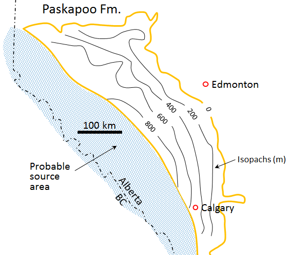
![Figure 21.32 The Tranquille Formation at the McAbee fossil site west of Kamloops, B.C. [SE]](http://opentextbc.ca/geology/wp-content/uploads/sites/110/2015/08/Tranquille-Formation-at-the-McAbee-fossil.jpg)
![Figure 21.33 Various glacial erosion features (top left) and glaciation at the Overlord Glacier, Coast Mountains, B.C. [Isaac Earle, used with permission]](http://opentextbc.ca/geology/wp-content/uploads/sites/110/2015/08/Various-glacial-erosion-features.jpg)
![Figure 21.34 A drumlin field with an esker (centre) in the Cree Lake area of northern Saskatchewan [NASA Landsat image, from Google Earth]](http://opentextbc.ca/geology/wp-content/uploads/sites/110/2015/08/drumlin-field-with-an-esker.png)

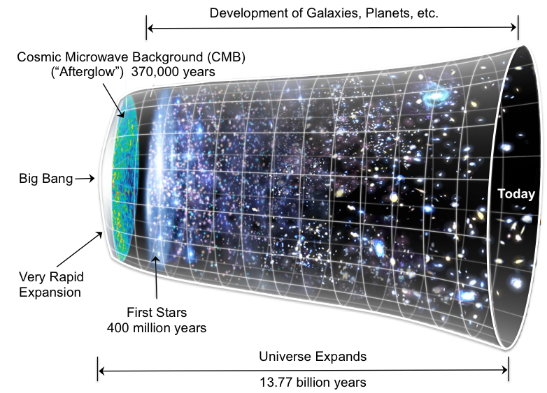
![Figure 22.2 Cosmic microwave background (CMB) map of the sky, a baby picture of the universe. The CMB is light from 375,000 years after the big bang. The colours reveal variations in density. Red patches have the highest density and blue patches have the lowest density. Regions of higher density eventually formed the stars, planets, and other objects we see in space today. [NASA/ WMAP Science Team http://bit.ly/CMBMap ]](https://opentextbc.ca/physicalgeologyearle/wp-content/uploads/sites/145/2016/03/cmwb-2.png)
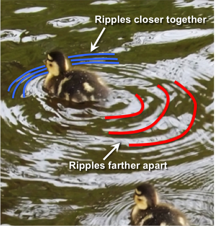

![Figure 22.5 Photograph of a nebula. The Pillars of Creation within the Eagle Nebula viewed in visible light (left) and near infrared light (right). Near infrared light captures heat from stars, and allows us to view stars that would otherwise be hidden by dust. This is why the picture on the right appears to have more stars than the picture on the left. [NASA, ESA, and the Hubble Heritage Team (STScI/AURA) http://bit.ly/1Dm2X5a]](http://opentextbc.ca/geology/wp-content/uploads/sites/110/2015/09/22.3.png)
![Figure 22.6 Public service announcement. If you don’t think housekeeping is important, then you don’t understand the gravity of the situation. [KP, with inspiration from NASA/JPL, http://1.usa.gov/1K1dVcU]](http://opentextbc.ca/geology/wp-content/uploads/sites/110/2015/09/22.6.png)
![Figure 22.7 Protoplanetary disks and Saturn’s rings. Upper left: An artists impression of a protoplanetary disk containing gas and dust, surrounding a new star. [NASA/ JPL-Caltech, http://1.usa.gov/1E5tFJR] Upper right: A photograph of the protoplanetary disk surrounding HL Tauri. The dark rings within the disk are thought to be gaps where newly forming planets are sweeping up dust and gas. [ALMA (ESO/NAOJ/NRAO) http://bit.ly/1KNCq0e]. Lower left: A photograph of Saturn showing similar gaps within its rings. The bright spot at the bottom is an aurora, similar to the northern lights on Earth. [NASA, ESA, J. Clarke (Boston University), and Z. Levay (STScI) http://bit.ly/1IfSCX5] Lower right: a close-up view of a gap in Saturn’s rings showing a small moon as a white dot. [NASA/JPL/Space Science Institute, http://1.usa.gov/1g2EeYw]](http://opentextbc.ca/geology/wp-content/uploads/sites/110/2015/09/22.7.png)
![Figure 22.8 Three types of planets. Jovian (or gas giant) planets such as Jupiter consist mostly of hydrogen and helium. They are the largest of the three types. Ice giant planets such as Uranus are the next largest. They contain water, ammonia, and methane ice. Terrestrial planets such as Earth are the smallest, and they have metal cores covered by rocky mantles. [KP, after public domain images by FrancescoA, WolfmanSF (http://bit.ly/1eP75P4), and NASA (http://1.usa.gov/1gFVsf6, http://1.usa.gov/1M89jI3)]](http://opentextbc.ca/geology/wp-content/uploads/sites/110/2015/09/22.8.png)
![Figure 22.9 Our solar system. Top: The solar system shown with distances to scale. Distances are in astronomical units (AU), where 1 AU is the average distance from Earth to the sun. The edge of the Kuiper belt extends to 50 AU (7.5 billion km), but this distance is miniscule compared to the size of the solar system as a whole, which extends to the edge of the Oort cloud, thought to be 15 trillion km away. Bottom: Solar system with sun and planets to scale. The gas giants are the largest planets, followed by the ice giants, and then the terrestrial planets. Note that the planets in this diagram likely do not reflect the entire population of planets in our solar system, because evidence suggests that large planets are present beyond the Kuiper belt. [KP, planet photographs courtesy of NASA via http://bit.ly/1M89xPs, Milky Way photo ForestWanderer (CC BY SA 3.0) http://bit.ly/1M89xPs]](http://opentextbc.ca/geology/wp-content/uploads/sites/110/2015/09/22.9.png)
![Figure 22.10 Photographs of Pluto. Left: The heart-shaped region called Tombaugh Regio is outlined. This region is named after Pluto’s discoverer Clyde Tombaugh [KP, NASA/APL/SwRI , http://1.usa.gov/1MOuT3m]. Right: False-colour images show compositional variations in Tombaugh Regio. [KP, NASA/APL/SwRI , http://1.usa.gov/1SO9bBu]](http://opentextbc.ca/geology/wp-content/uploads/sites/110/2015/09/22.10.png)
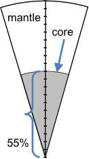
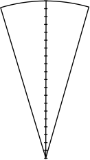
![Figure 22.11 Artist’s impression of a collision between planets. A similar collision between Earth and the planet Theia might have given us our moon. Fortunately for us, the collision that gave us the moon was a glancing blow rather than the direct hit shown here. Earth might not have survived a direct hit. [NASA/ JPL-Caltech, http://1.usa.gov/1IkP069]](http://opentextbc.ca/geology/wp-content/uploads/sites/110/2015/09/22.11.png)
![Plot showing how the star Kepler-452 dims as the planet Kepler-452b moves in front of it. [KP, after Jenkins, J. et al, 2015, Discovery and validation of Kepler-452b: a 1.6REarth super Earth exoplanet in the habitable zone of a G2 star, Astronomical Journal, V 150, DOI 10.1088/0004-6256/150/2/56.]](http://opentextbc.ca/geology/wp-content/uploads/sites/110/2015/09/exercise-22.2.png)
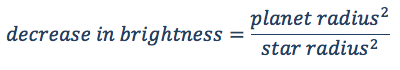
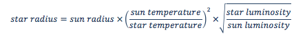
![Spectra for the sun and two galaxies. [KP]](http://opentextbc.ca/geology/wp-content/uploads/sites/110/2015/09/spectraforsun.png)
![Denizens of the solar system. [Randall Munroe (CC BY-NC 2.5) https://xkcd.com/1297/]](http://opentextbc.ca/geology/wp-content/uploads/sites/110/2015/09/denizens.png)
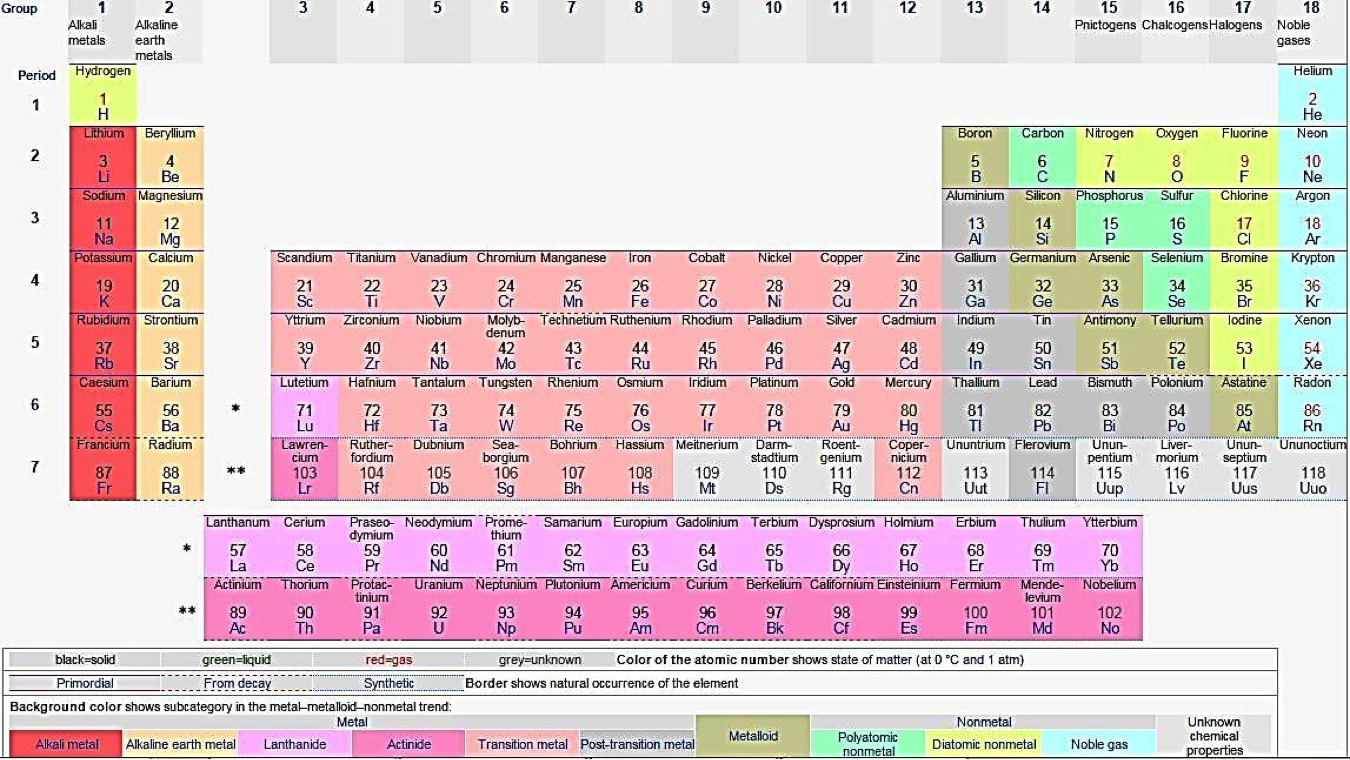
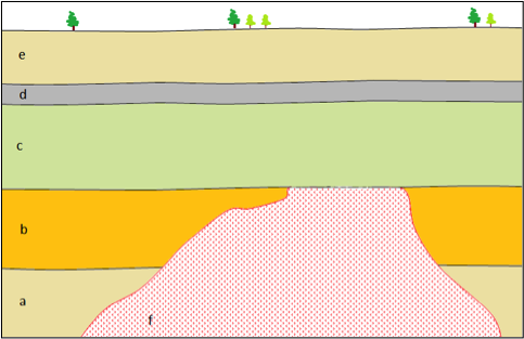
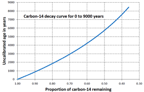
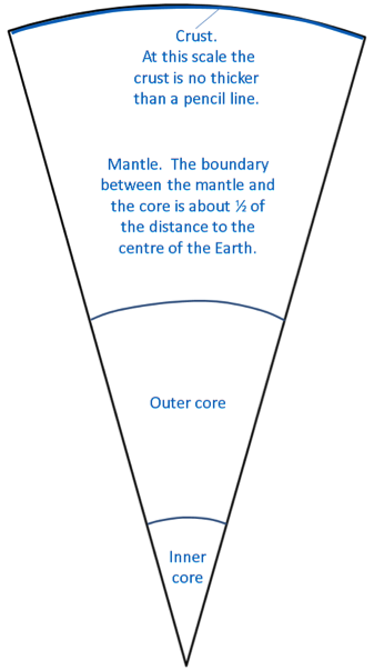
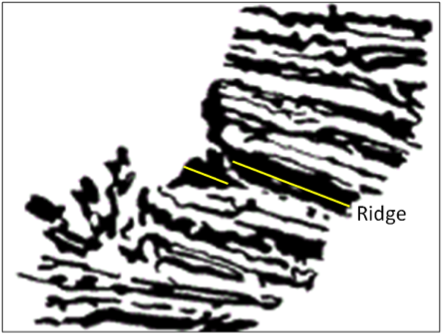


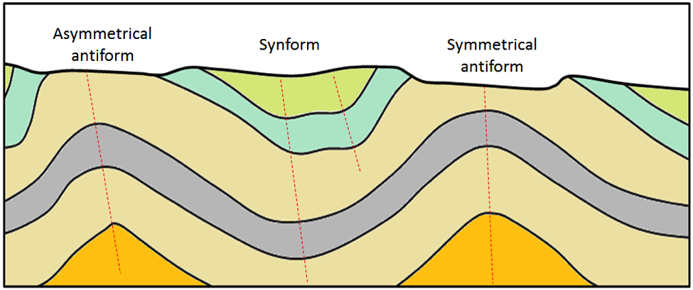
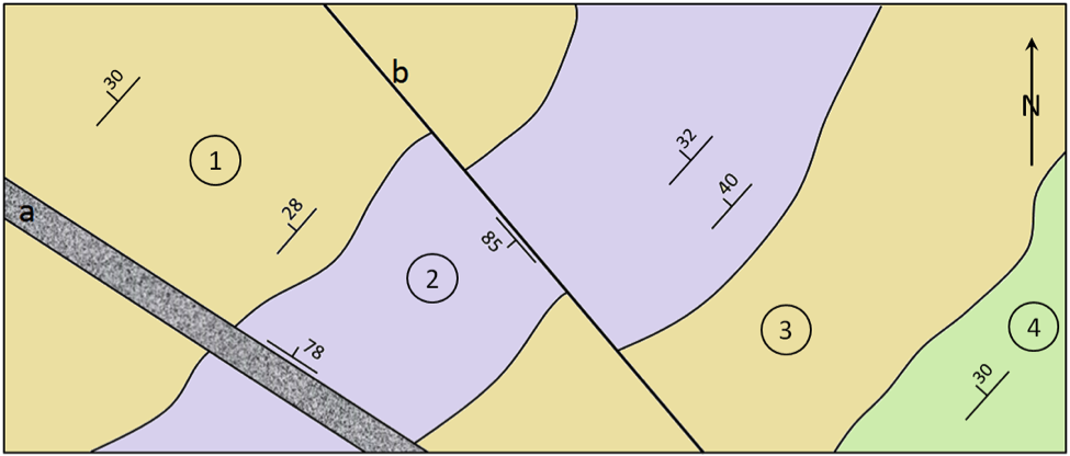
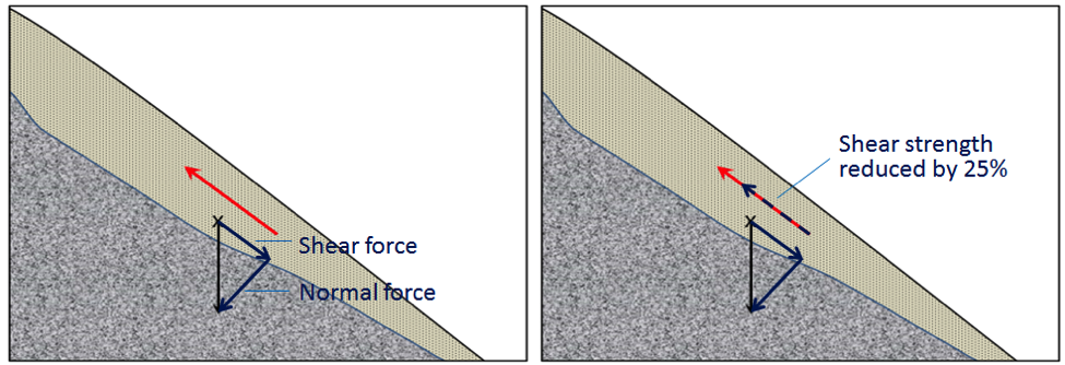
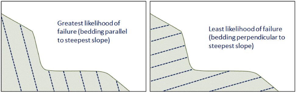

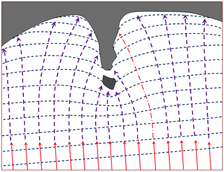
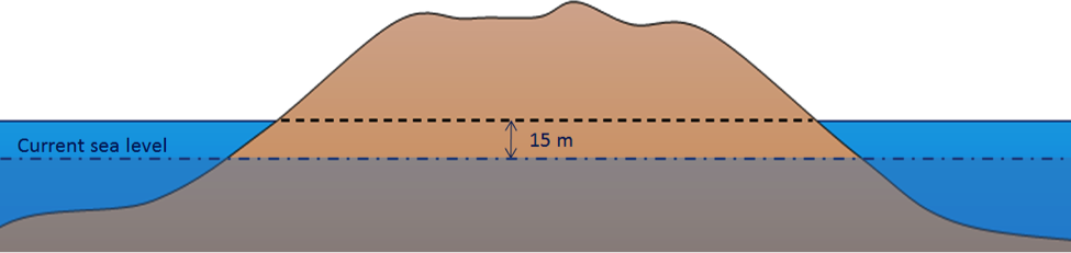
![Spectra for the sun and two galaxies. [KP]](http://opentextbc.ca/geology/wp-content/uploads/sites/110/2015/09/spectra.png)
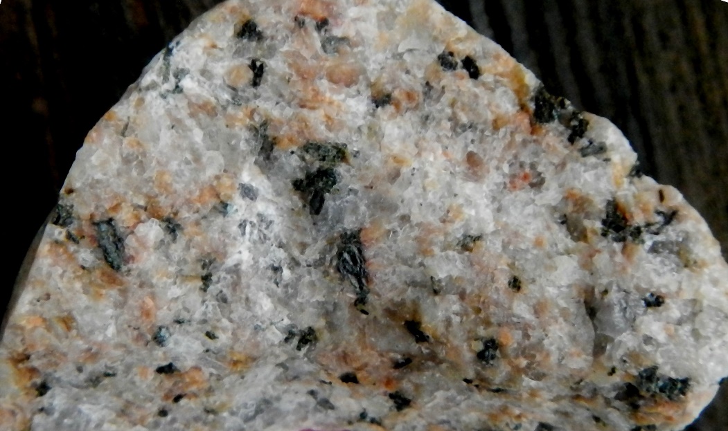
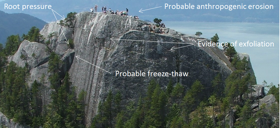
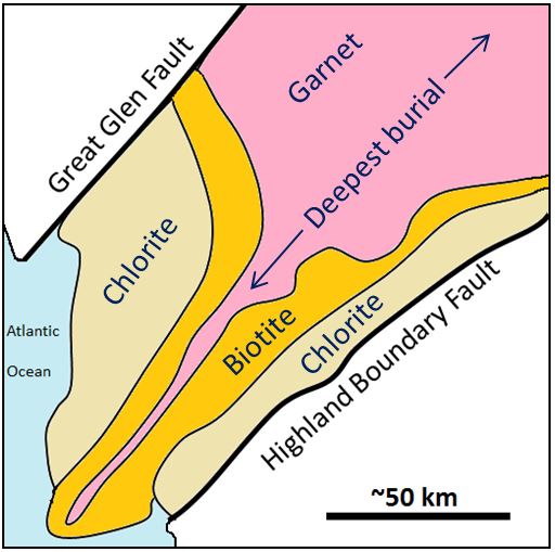

![Relative ages: 2: oldest: 3: middle, 1: youngest [SE]](https://opentextbc.ca/physicalgeologyearle/wp-content/uploads/sites/145/2016/07/ex8-1.png)
![Dating from overlapping fossils [SE]](https://opentextbc.ca/physicalgeologyearle/wp-content/uploads/sites/145/2016/07/ex8-2.png)
![Isotopic dating [SE]](https://opentextbc.ca/physicalgeologyearle/wp-content/uploads/sites/145/2016/07/ex8-3.png)
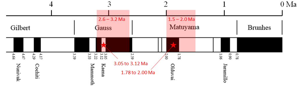
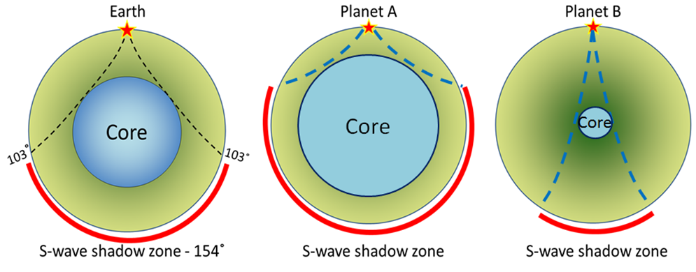
![Rock densities [SE]](https://opentextbc.ca/physicalgeologyearle/wp-content/uploads/sites/145/2016/07/ex9-4.png)
![Pangea [SE]](https://opentextbc.ca/physicalgeologyearle/wp-content/uploads/sites/145/2016/07/ex10-1.png)
![Pacific Plate rates of motion [SE]](https://opentextbc.ca/physicalgeologyearle/wp-content/uploads/sites/145/2016/07/ex10-2.png)
![Juan de Fuca and Explorer Plates [SE]](https://opentextbc.ca/physicalgeologyearle/wp-content/uploads/sites/145/2016/07/ex10-4.png)
![The extents of the Earth's major plates [SE]](https://opentextbc.ca/physicalgeologyearle/wp-content/uploads/sites/145/2016/07/ex10-5.png)
![[SE from Earthquakes Canada at http://www.earthquakescanada.nrcan.gc.ca/index-en.php]](https://opentextbc.ca/physicalgeologyearle/wp-content/uploads/sites/145/2016/07/ex11-1.png)
![Folded rocks (outlined in yellow) and fold axes (pink) [SE]](https://opentextbc.ca/physicalgeologyearle/wp-content/uploads/sites/145/2016/07/ex12-1.png)
![Vertical cross section (above), map view (below) [SE]](https://opentextbc.ca/physicalgeologyearle/wp-content/uploads/sites/145/2016/07/ex12-3.png)
![[SE]](https://opentextbc.ca/physicalgeologyearle/wp-content/uploads/sites/145/2016/07/ex13-3.png)
![Gradients of Priest Creek [SE]](https://opentextbc.ca/physicalgeologyearle/wp-content/uploads/sites/145/2016/07/ex13-4.png)
![[BC Ministry of the Environment at http://www.env.gov.bc.ca/wsd/data_searches/obswell/map/]](https://opentextbc.ca/physicalgeologyearle/wp-content/uploads/sites/145/2016/07/ex14-3.png)
![Implications of pumping from wells B and C and injecting into well A [SE]](https://opentextbc.ca/physicalgeologyearle/wp-content/uploads/sites/145/2016/07/ex14-6.png)
![[SE]](https://opentextbc.ca/physicalgeologyearle/wp-content/uploads/sites/145/2016/07/ex15-2.png)
![[SE]](https://opentextbc.ca/physicalgeologyearle/wp-content/uploads/sites/145/2016/07/ex16-1.png)
![Glacial advance (top) and retreat (bottom) [SE]](https://opentextbc.ca/physicalgeologyearle/wp-content/uploads/sites/145/2016/07/ex16-2.png)
![[SE after http://en.wikipedia.org/wiki/Mount_Assiniboine#/media/File:Mount_Assiniboine_Sunburst_Lake.jpg]](https://opentextbc.ca/physicalgeologyearle/wp-content/uploads/sites/145/2016/07/ex16-3.png)
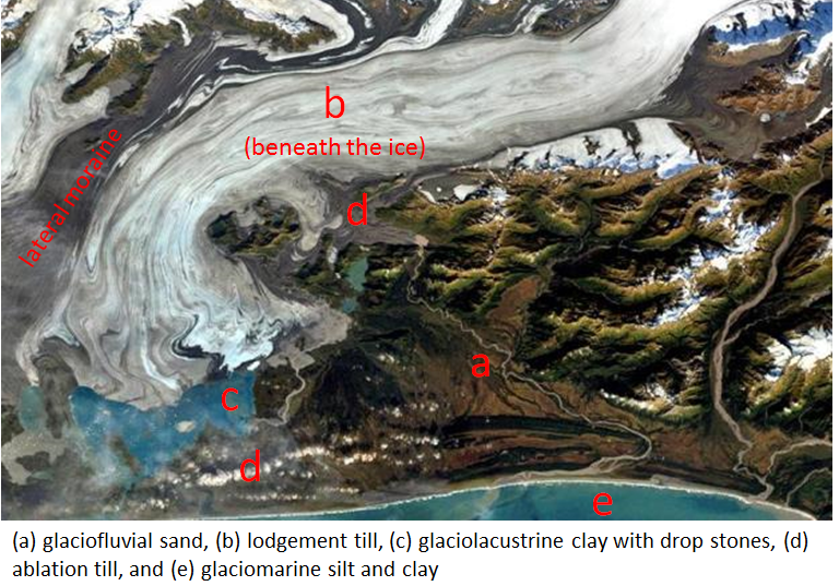
![[SE]](https://opentextbc.ca/physicalgeologyearle/wp-content/uploads/sites/145/2016/07/ex17-2.png)
![Possible locations of coastal deposits [SE]](https://opentextbc.ca/physicalgeologyearle/wp-content/uploads/sites/145/2016/07/ex17-3.png)
![[SE]](https://opentextbc.ca/physicalgeologyearle/wp-content/uploads/sites/145/2016/07/ex17-5.png)
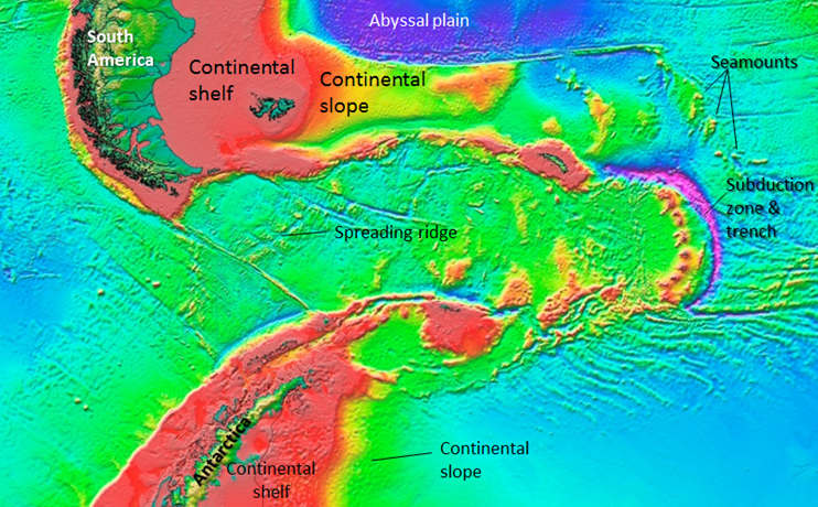
![[SE]](https://opentextbc.ca/physicalgeologyearle/wp-content/uploads/sites/145/2016/07/ex18-2.png)
![[SE]](https://opentextbc.ca/physicalgeologyearle/wp-content/uploads/sites/145/2016/07/ex18-3.png)
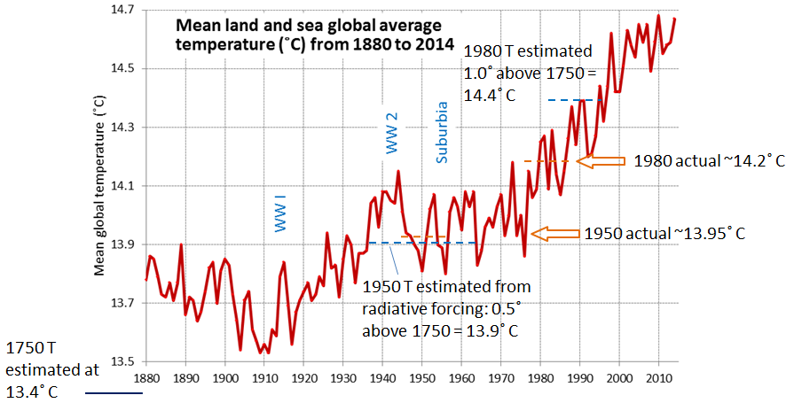
![[SE using climate data from Environment Canada, and ENSO data from: http://www.esrl.noaa.gov/psd/enso/mei/table.html]](https://opentextbc.ca/physicalgeologyearle/wp-content/uploads/sites/145/2016/07/ex19-4.png)
![[SE after USGS at: http://walrus.wr.usgs.gov/infobank/programs/html/definition/seis.html]](https://opentextbc.ca/physicalgeologyearle/wp-content/uploads/sites/145/2016/07/ex20-4.png)
![[SE after Geological Survey of Canada]](https://opentextbc.ca/physicalgeologyearle/wp-content/uploads/sites/145/2016/07/ex21-1.png)
![[SE]](https://opentextbc.ca/physicalgeologyearle/wp-content/uploads/sites/145/2016/07/ex21-3.png)
![[KP]](https://opentextbc.ca/physicalgeologyearle/wp-content/uploads/sites/145/2016/07/ex22-1.png)
![[KP, after Jenkins, J. et al, 2015, Discovery and validation of Kepler-452b: a 1.6REarth super Earth exoplanet in the habitable zone of a G2 star, Astronomical Journal, V 150, DOI 10.1088/0004-6256/150/2/56.]](https://opentextbc.ca/physicalgeologyearle/wp-content/uploads/sites/145/2016/07/ex22-2.png)
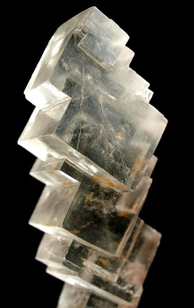
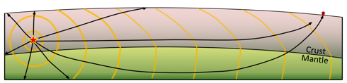
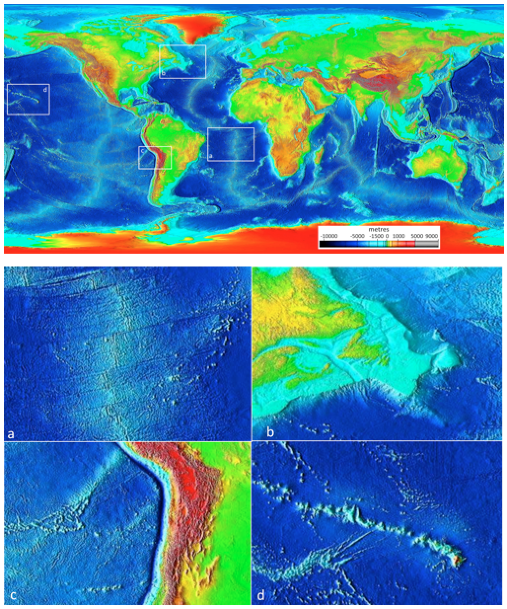
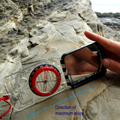