Cover Page
The illustrators of the cover page were Sarah Nersesian and Anupreet Kharbanda of Designs that Cell.
Meet the Authors
The illustrators of the author images were Sarah Nersesian and Anupreet Kharbanda of Designs that Cell.
1 – Stoichiometry
1.1 – The Mole
This chapter contains material and exercises taken from Section 3.1 “Formula Mass and the Mole Concept” and its exercises, respectively, of the open textbook resource Chemistry 2e (on OpenStax) by Flowers, Theopold, Langley, and Robinson, PhD, used under a CC BY 4.0 license, including:
Paragraphs 1-7,
Examples 1.1.1, 1.1.2, 1.1.3, 1.1.4, 1.1.5 and 1.1.6,
“Check your learning” 1.1.1, 1.1.2, 1.1.3, 1.1.4, 1.1.5 and 1.1.6, and
Table 1.1.1.
This chapter also contains material taken from Section 1.5 “Density and Percent Composition: Their Use in Problem Solving” of the Chemistry Libretexts textmap for General Chemistry: Principles and Modern Applications (by Petrucci et al.) as part of the Open Education Resource (OER) LibreTexts Project, used under a CC BY-NC-SA 3.0 license, including:
Paragraph 10, and
Example 1.1.7.
This chapter contains content taken from 3.2 – Determining Empirical and Molecular Formulas, including paragraphs 8 and 9.
This chapter contains material taken from Section 3.1 “Formula Mass and the Mole Concept” of the open textbook resource Chemistry 2e (on OpenStax) by Flowers, Theopold, Langley, and Robinson, PhD, used under a CC BY 4.0 license including the end of section 1.1 questions and its answers.
This chapter contains original material by Jessica Thomas including the material in the brackets of example 1.1.1 and the answers for the end of section 1.1 questions 1 and 7.
This chapter contains original material by Leanne Trepanier and Nathan Biniam including the answers to the end of section 1.1 questions 5 and 8.
This chapter contains original content by Geneviève O’Keefe and Derek Fraser-Halberg including the numbering of figures, examples and tables.
This chapter contains figures 1.1.1, 1.1.2, 1.1.3 and 1.1.4 taken from 3.1 – Formula Mass and the Mole Concept.
1.2 – Determining Chemical Formulae
This chapter contains material and exercises taken from the following sections of the open textbook resource Chemistry 2e (on OpenStax) by Flowers, Theopold, Langley, and Robinson, PhD:
Section 2.3 “Atomic Structure and Symbolism,”
The “In case you’re interested … Mass Spectrometry” box
Section 2.4 “Chemical Formulas” and its exercises,
Paragraphs 2-6 and 11,
Section 3.2 “Determining Empirical and Molecular Formulas” and its exercises,
Paragraphs 12-16 and 18-23,
Examples 1.2.1, 1.2.2 and 1.2.4,
“Check your learning” 1.2.1 and 1.2.2,
Section 4.1 “Writing and Balancing Chemical Equations” and its exercises,
Paragraphs 24-33,
The “Balancing Chemical equations – additional practice” box,
Section 4.5 “Quantitative Chemical Analysis,”
Paragraph 17,
Examples 1.2.3 and 1.2.5,
“Check your learning” 1.2.3 and 1.2.7,
all used under a CC BY 4.0 license.
This chapter also contains an exercise taken from Section 1.3 “Introduction to Combustion Analysis” of the open textbook resource Physical Methods in Chemistry and Nano Science (by Raja and Barron) as part of the Open Education Resource (OER) LibreTexts Project, used under a CC BY 4.0 license.
This chapter also contains an example and exercises taken from the exercises of Section 3 “Stoichiometry” of the Chemistry Libretexts textmap for Chemistry: The Central Science (by Brown, LeMay, Busten, Murphy, and Woodward) as part of the Open Education Resource (OER) LibreTexts Project, used under a CC BY-NC-SA 4.0 license.
This chapter contains example 1.2.4 taken from 3.2 – Determining Empirical and Molecular Formulas.
This chapter contains end of section 1.2 questions 1 and 2 and its answers taken from Section 2.4 “Chemical Formulas” of the open textbook resource Chemistry 2e (on OpenStax) by Flowers, Theopold, Langley, and Robinson, PhD, used under a CC BY 4.0 license.
This chapter contains end of section 1.2 questions 3-6 and its answers taken from Section 3.2 “Determining Empirical and Molecular Formulas” of the open textbook resource Chemistry 2e (on OpenStax) by Flowers, Theopold, Langley, and Robinson, PhD, used under a CC BY 4.0 license.
This chapter contains end of section 1.2 questions 7 and 8, and its answers taken from Exercises 3. E “Stoichiometry (Exercises)” of the Chemistry Libretexts textmap for Chemistry: The Central Science (by Brown, LeMay, Busten, Murphy, and Woodward) as part of the Open Education Resource (OER) LibreTexts Project, used under a CC BY-NC-SA 4.0 license.
This chapter contains end of section 1.2 question 9-11 and its answers taken from Section 4.1 “Writing and Balancing Chemical Equations” of the open textbook resource Chemistry 2e (on OpenStax) by Flowers, Theopold, Langley, and Robinson, PhD, used under a CC BY 4.0 license.
This chapter contains original material written by Dr. Brandi West including the paragraph under the answer of “Check your learning” 1.2.6.
This chapter includes original material written by Mahdi Zeghal including paragraph 1 and 7-9, brackets in the second sentence of paragraph 3, brackets in the first sentence of paragraph 4, brackets in the second sentence of paragraph 6, brackets in the fourth sentence of paragraph 11, brackets of the first sentence in paragraph 17, the “combustion analysis problems – underlying assumption” box, the third paragraph under the solution of “Check your learning” 1.2.4 and the first sentence in the “Balancing Chemical equations – additional practice” box.
This chapter contains original material by Geneviève O’Keefe including the fourth sentence in paragraph 6 and paragraph 10.
This chapter contains original material by Leanne Trepanier and Nathan Biniam including the answers to the end of section 1.2 questions 5 and 11.
This chapter contains original content by Geneviève O’Keefe and Derek Fraser-Halberg including the numbering of figures, and examples.
This chapter contains figure 1.2.9 taken from “Atomic Structure and Symbolism.”
This chapter contains figures 1.2.1, 1.2.2, 1.2.3 and 1.2.4 taken from “Chemical Formulas.”
This chapter contains figures 1.2.5, 1.2.6 and 1.2.7 taken from “Determining Empirical and Molecular Formulas.”
This chapter contains figures 1.2.11 and 1.2.12 taken from “Writing and Balancing Chemical Equations.”
This chapter contains figure 1.2.8 taken from “Quantitative Chemical Analysis.”
1.3 – Reaction Stoichiometry
This chapter contains material and exercises taken from the following sections of the open textbook resource Chemistry 2e (on OpenStax) by Flowers, Theopold, Langley, and Robinson, PhD:
Section 4.3 “Reaction Stoichiometry” and its exercises,
Paragraphs 1-8,
Examples 1.3.1, 1.3.2, 1.3.3, 1.3.4,
“Check your learning” 1.3.4,
End of chapter 1.3 questions 1-8, and
Section 4.4 “Reaction Yields” and its exercises,
Paragraphs 9-15,
Examples 1.3.5, and 1.3.6,
“Check your learning” 1.3.5 (a), and
End of chapter 1.3 questions 9-12,
both used under a CC BY 4.0 license.
This chapter contains original content created by Jessica Thomas including example 1.3.5 question and answer for b, and the question and answer for example 1.3.6.
This chapter contains original answers for questions 1, 2, 5, 6, 8, 9, 10 and 12 created by Nathan Biniam and Leanne Trepanier.
This chapter contains original content by Geneviève O’Keefe including the numbering of certain figures and the answer to question 5 at the end of this section.
This chapter contains original content by Derek Fraser-Halberg including the numbering of figures and equations.
This chapter contains figures 1.3.1 and 1.3.2 taken from Section 4.3 “Reaction Stoichiometry.”
This chapter contains figures 1.3.3 and 1.3.4 taken from Section 4.4 “Reaction Yields.”
1.4 – Solution Stoichiometry
This chapter contains material and exercises taken from Section 3.3 “Molarity” and its exercises, respectively, of the open textbook resource Chemistry 2e (on OpenStax) by Flowers, Theopold, Langley, and Robinson, PhD, used under a CC BY 4.0 license, including:
Paragraphs 1-5 and 19-22,
Examples 1.4.1, 1.4.2, 1.4.3, 1.4.4, 1.4.5, 1.4.11, 1.4.12, 1.4.13, and
“Check your learning” 1.4.1, 1.4.2, 1.4.3, 1.4.4, 1.4.5, 1.4.11, 1.4.12, and 1.4.13.
This chapter also contains material taken from the following open textbook resources of the Open Education Resource (OER) LibreTexts Project:
“Fundamental Characteristics of Water,” a section of Aquatic Chemistry (by Chieh) of the Chemistry Libretexts supplemental modules on environmental chemistry, used under a CC BY-NC-SA 3.0 license,
Paragraphs 17 and 18,
Section 7.6 “Writing Chemical Equations for Reactions in Solution- Molecular, Complete Ionic, and Net Ionic Equations,” a section of the Chemistry Libretexts textmap for Introductory Chemistry (by Tro), used under a CC BY-NC-SA 3.0 license,
Paragraphs 24-29,
Examples 1.4.14 and 1.4.16,
“Check your learning” 1.4.15 and 1.4.16, and
Section 16.11 “Molality,” a section of Introductory Chemistry (CK-12), used under a CC BY-NC 4.0 license,
Paragraphs 14-16, and
Example 1.4.10.
This chapter contains original content by Dr. Brandi West including the second sentence of paragraph 24.
This chapter contains original content by Jessica Thomas including sentence 2 in paragraph 9, the sentence in example 1.4.6 above the subtitle “Check your learning”, the question and answer for (a) in “Check your learning” 1.4.9, the last sentence in paragraph 20, the 3 first numbered points under “Molecular, complete ionic, and net equations” and the end of chapter questions from 8 to 16.
This chapter contains original answers for questions 7 to 18 created by Nathan Biniam and Leanne Trepanier.
This chapter contains the equation for point 1 under “Molecular, complete ionic, and net equations” (Acid-Base Reactions).
This chapter contains the equation for point 2 under “Molecular, complete ionic, and net equations” (5.6 – Oxidation-Reduction (Redox) Reactions).
This chapter contains an exercise and its answer for the end of chapter question 21 taken from Section 4.2 “Classifying Chemical Reactions” of the open textbook resource Chemistry 2e (on OpenStax) by Flowers, Theopold, Langley, and Robinson, PhD, used under a CC BY 4.0 license.
This chapter contains original content by Geneviève O’Keefe and Derek Fraser-Halberg including the numbering of figures and equations.
This chapter contains figures and material from (3.4 – Other Units for Solution Concentrations) including figures 1.4.3, 1.4.4, 1.4.5 and 1.4.7 and paragraphs 6 and 8 to 13, first sentence in paragraph 1, examples 1.4.6, 1.4.7, 1.4.8, and 1.4.9, and “Check your learning” 1.4.6, 1.4.7, 1.4.8, and 1.4.9 (b).
This chapter contains figures 1.4.1, 1.4.2, and 1.4.6 taken from “Molarity.”
This chapter contains figures 1.4.8 taken from “Writing Chemical Equations for Reactions in Solution- Molecular, Complete Ionic, and Net Ionic Equations.”
1.5 – Redox Reactions
This chapter contains material and exercises taken from the following sections of the open textbook resource Chemistry 2e (on OpenStax) by Flowers, Theopold, Langley, and Robinson, PhD:
Section 4.2 “Classifying Chemical Reactions” and its exercises,
Paragraphs 1-3 and 5-9,
Examples 1.5.1 and 1.5.2,
“Check your learning” 1.5.1 and 1.5.2, and
Section 17.1 “Review of Redox Chemistry” and its exercises,
Examples 1.5.3 and 1.5.5, and
“Check your learning” 1.5.4 and 1.5.5,
both used under a CC BY 4.0 license.
This chapter contains original content by Mahdi Zeghal including:
Sentences within steps of example 1.5.5,
“Tips and Tricks – oxidation and reduction acronyms”,
In paragraph 5: The “(e.g)” for points 1, 2, and 4, and the last part of the sentence, under bullet point 4, after the last comma in both points 4.2 and 4.3,
Paragraph 6,
Sentence 1 and 5 in paragraph 10, as well as steps 1 and 9, and
“Note” in example 1.5.3 and the sentence in example 1.5.3 about step 7 of the example’s solution.
This chapter contains original content by Geneviève O’Keefe including the second and last sentence in paragraph 1.
This chapter contains original content by Geneviève O’Keefe and Derek Fraser-Halberg including the numbering of figures and equations.
This chapter contains original answers for questions 1, 3, 5, 10 and 11 created by Nathan Biniam and Leanne Trepanier.
This chapter contains figure 1.5.2 taken from “Classifying Chemical Reactions.”
Chapter 1 Key Terms
The definitions for the following key terms were adapted from the Chapter 2 Key Terms of the open textbook resource Chemistry 2e (on OpenStax) by Flowers, Theopold, Langley, and Robinson, PhD, used under a CC BY 4.0 license:
|
Empirical formula
|
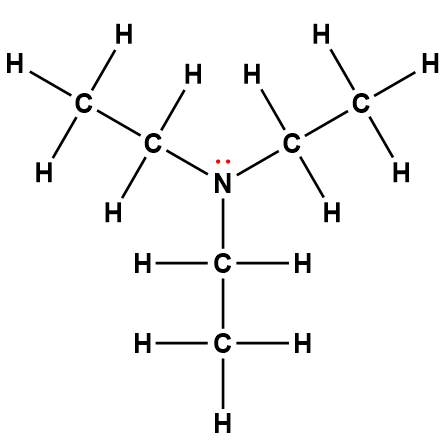
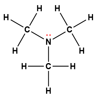
Isomers
|
Molecular formula
|
Structural formula
|
|
|
|
|
The definitions for the following key terms were adapted from the Chapter 3 Key Terms of the open textbook resource Chemistry 2e (on OpenStax) by Flowers, Theopold, Langley, and Robinson, PhD, used under a CC BY 4.0 license:
|
Aqueous solution
|
Dilution
|
Molarity (M)
|
Solute
|
|
Avogadro’s number (NA)
|
Empirical formula mass
|
Mole (n)
|
Solvent
|
|
Concentrated
|
Mass percentage (m/m %)
|
Parts per billion (ppb)
|
Volume percentage (v/v %)
|
|
Concentration (C)
|
Mass-volume percent (m/v %)
|
Parts per million (ppm)
|
|
|
Dilute
|
Molar mass (Mm)
|
Percent composition
|
|
|
|
|
|
The definitions for the following key terms were adapted from the Chapter 4 Key Terms of the open textbook resource Chemistry 2e (on OpenStax) by Flowers, Theopold, Langley, and Robinson, PhD, used under a CC BY 4.0 license:
|
Actual yield
|
Excess reactant
|
Percent yield
|
Spectator ion
|
|
Balanced equation
|
Limiting reactant
|
Precipitation reaction
|
Stoichiometric factor
|
|
Coefficient
|
Net ionic equation
|
Product
|
Stoichiometry
|
|
Combustion analysis
|
Oxidation number
|
Reactant
|
Theoretical yield
|
|
Combustion reaction
|
Oxidation-reduction reaction
|
Reducing agent
|
|
|
Complete ionic equation
|
Oxidizing agent
|
Single-displacement reaction
|
|
|
|
|
|
The definitions for the following key terms were adapted from the Chapter 11 Key Terms of the open textbook resource Chemistry 2e (on OpenStax) by Flowers, Theopold, Langley, and Robinson, PhD, used under a CC BY 4.0 license:
The definitions for the following key terms were adapted from the Glossary of the open textbook resource Introductory Chemistry – 1st Canadian Edition (by Key and Ball), used under a CC BY-NC-SA 4.0 license:
|
Chemical equation
|
Dilute
|
Mole (n)
|
Reduction
|
|
Coefficient
|
Half-reaction
|
Oxidation
|
Single-displacement reaction
|
|
Combustion reaction
|
Half-reaction method
|
Oxidation-reduction reaction
|
Solute
|
|
Concentration
|
Limiting reactant
|
Percent yield
|
Solvent
|
|
|
|
|
The definitions for the following key terms were adapted from another open textbook resource of the Open Education Resource (OER) LibreTexts Project:
Hydrophilic and hydrophobic – from “Fundamental Characteristics of Water,” a section of Aquatic Chemistry (by Chieh) of the Chemistry Libretexts supplemental modules on environmental chemistry, used under a CC BY-NC-SA 3.0 license.
2 – Gases
2.1 – Intermolecular Forces
This chapter contains material and exercises taken from the following sections of the open textbook resource Chemistry 2e (on OpenStax) by Flowers, Theopold, Langley, and Robinson, PhD:
Section 10.1 “Intermolecular Forces” and its exercises,
Paragraphs 1-22,
Example 2.1.1,
“Check your learning” 2.1.1 – 2.13,
Figures 2.1.1 – 2.1.13, and
Questions and Answers 2, 5, 6 and 7.
This chapter also contains material taken from the following open textbook resources of the Open Education Resource (OER) LibreTexts Project:
Section 3.7 “Intermolecular forces,” a unit section of the course CHEM1130 Principles of Chemistry I (from the Northern Alberta Institute of Technology), used under a CC BY-NC-SA 3.0 license,
Paragraph 23,
Questions 1, 3, and 4, and
Answers 1, 2, 3, 4, 5, 6, and 7.
This chapter contains original content by Dr. Kathy-Sarah Focsaneanu including:
Sentence 3 in paragraph 3,
Sentence 4 in paragraph 16, and
Answer for “Check your learning” 2.1.3.
This chapter contains original content by Jessica Thomas including:
Summary at the end of chapter.
This chapter contains original content by Geneviève O’Keefe and Derek Fraser-Halberg including the numbering of figures and equations.
This chapter contains original answers for questions 5 created by Nathan Biniam and Leanne Trepanier.
2.2 – Gases and the Periodic Table
This chapter contains material taken from Section 10.1 “Characteristics of Gases” of the Chemistry Libretexts textmap for Chemistry: The Central Science (by Brown, LeMay, Busten, Murphy, and Woodward) as part of the Open Education Resource (OER) LibreTexts Project, used under a CC BY-NC-SA 4.0 license, including:
Paragraphs 1-3,
Examples,
“Check your learning”, and
Figure 2.2.1.
This chapter contains original content by Jessica Thomas and Dr. Kathy-Sarah Focsaneanu including:
Questions and answers 1 and 2.
2.3 – Measuring Variables of Gases
This chapter contains material and/or examples taken from the following open textbook resources of the Open Education Resource (OER) LibreTexts Project:
Section 2.2 “Expressing Units,” a section of Beginning Chemistry (by Ball), used under a CC BY-NC-SA 4.0 license,
Paragraphs 18-19,
Figure 2.3.5, and
Section 2.4 “Temperature,” a unit section of the course CHM101: Chemistry and Global Awareness (by Gordon from Furman University), used under a CC BY-NC-SA 4.0 license,
Paragraphs 20-26,
Example 2.3.6,
Figure 2.3.6, and
Section 5.2 “Gas Pressure and Its Measurement,” a section of the Chemistry Libretexts textmap for Chemistry – The Molecular Nature of Matter and Change (by Silberberg), used under a CC BY-NC-SA 3.0 license,
Paragraphs 8-16
Examples 2.3.4, 2.3.5,
Figures 2.3.2, 2.3.3, 2.3.4,
“Check your learning” 2.3.3, 2.3.4, 2.3.5, and
Sections 9.3 “Pressure” and 9.4 “Measurement of Pressure,” sections of ChemPRIME (by Moore et al.), both used under a CC BY-NC-SA 4.0 license,
Paragraphs 1-7,
Examples 2.3.1, 2.3.3,
Figure 2.3.1,
“Check your learning” 2.3.2, and
Questions 8 and 9.
This chapter contains original content by Dr. Kathy-Sarah Focsaneanu including:
Changes made on paragraphs 9, 12, 15, 18, and 23, and
End of the chapter questions 1, 2, 3, 5, 6, and 11.
This chapter contains original content by Derek Fraser-Halberg including:
End of the chapter answers.
This chapter contains original content by Mahdi Zeghal including:
Subheading for figure 2.3.1.
This chapter contains original content by Leanne Trepanier and Derek Fraser-Halberg including the numbering of figures and equations.
2.4 – Gas Laws
This chapter contains material and exercises taken from Section 9.2 “Relating Pressure, Volume, Amount, and Temperature: The Ideal Gas Law” and its exercises, respectively, of the open textbook resource Chemistry 2e (on OpenStax) by Flowers, Theopold, Langley, and Robinson, PhD, used under a CC BY 4.0 license, including:
Paragraphs 1-25,
Examples 2.4.1 – 2.4.6,
Figures 2.4.1 – 2.4.10,
“Check your Learning” 2.4.1 – 2.4.6,
Questions 1-14, and
Answers 11 and 14.
This chapter contains original content by Dr. Kathy-Sarah Focsaneanu including:
Changes to titles, equations and figures.
This chapter contains original content by Leanne Trepanier and Geneviève O’Keefe including the numbering of equations, figures and answers 1, 3, 4, 5, 7, 9, and 10.
This chapter contains original content by Mahdi Zeghal including change to the CHEM1311 Laboratory section.
This chapter contains original answers for questions 2, 6, 8, 12 and 13 created by Nathan Biniam.
2.5 – Gas Mixtures and Partial Pressures
This chapter contains material and exercises taken from the following sections of the open textbook resource Chemistry 2e (on OpenStax) by Flowers, Theopold, Langley, and Robinson, PhD:
Section 9.3 “Stoichiometry of Gaseous Substances, Mixtures, and Reactions” and its exercises,
Paragraphs:
Under Equation 2.5.1 (Whole paragraph),
Paragraph 4 Sentence 2,
Paragraph 5 (Whole paragraph),
Paragraph 6 (Whole paragraph),
Paragraph 7 (Whole paragraph),
Examples,
Figure 2.5.1, and
“Check your learning”.
2.6 – Kinetic-Molecular Theory of Gases (Ideal Gas Behaviours)
This chapter contains material and exercises taken from the following sections of the open textbook resource Chemistry 2e (on OpenStax) by Flowers, Theopold, Langley, and Robinson, PhD:
Section 9.5 “The Kinetic-Molecular Theory” and its exercises,
Paragraphs 1-12,
Example 2.6.1,
Figures 2.6.1, 2.6.2, 2.6.3, 2.6.4, 2.6.5, and
“Check your Learning” 2.6.1.
This chapter contains original content by Leane Trapier and Derek Fraser-Halberg including numbering of equations and equation subheadings.
This chapter contains original content by Jessica Thomas including:
Sentence 1 from paragraph 9 (added “where M is the average mass of the particles”),
Paragraph 10 (added “(to extend your learning, check out the derivation for KEavg here):”),
Sentence 1 of the answer to “Check your learning” 2.6.1, and
Questions 1-8.
This chapter contains original content by Geneviève O’Keefe including:
Inserting “decrease both” to Charles’s Law – sentence 3, and
Answers 2, 5 and 7.
This chapter contains original content by Dr. Kathy-Sarah Focsaneanu including:
Added “Gay-Lussac’s law” to “ The Kinetic-Molecular Theory Explains the Behavior of Gases, Part I – Amontons’ ”,
Added a paragraph under equation 2.6.2, and
Added “expressed in kilograms” to paragraph 9.
This chapter contains original content by Nathan Biniam including:
End of chapter answers 1, 3, 4, 6, and 8.
2.7 – Diffusion and Effusion
This chapter contains material and exercises taken from the following sections of the open textbook resource Chemistry 2e (on OpenStax) by Flowers, Theopold, Langley, and Robinson, PhD:
Section 9.4 “Effusion and Diffusion of Gases” and its exercises,
Paragraphs 1-10,
Examples 2.7.1, 2.7.2, 2.7.3,
Figures 2.7.1, 2.7.2, 2.7.3, and
“Check your Learning” 2.7.1, 2.7.2, 2.73.
This chapter contains original content by Genevieve O’Keefe including:
First two sentences in paragraph 1,
Paragraph 6 sentence 1,
Example 2.7.3,
Paragraph 1 Sentence 3,
Solution – Sentence 4,
Above “Check your Learning” 2.7.3, Paragraph was added,
Wrote “In Case You’re Interested… Use of Diffusion for Nuclear Energy Applications: Uranium Enrichment” Section, and
Answers for questions 1, 3, 5, 7, and 9.
This chapter contains original content by Jessica Thomas including:
Questions 1 to 9.
This chapter contains original content by Mahdi Zeghal including:
Added to sentence 1 in the section “The Kinetic-Molecular Theory Explains the Behavior of Gases, Part II,
Example 2.7.3 “Elements and Molar Masses”, and
Answer for question 6.
This chapter contains original content by Leanne Trepanier including:
Answers for questions 2, 3, 4, 8, and
Edit to questions 1 and 8.
This chapter contains original content by Dr. Kathy-Sarah Focsaneanu including:
Paragraph 7,
Example 2.7.1,
Added a couple words to the first paragraph, and
Whole solution (else than the equation).
This chapter contains original content by Leane Trapier and Derek Fraser-Halberg including numbering of equations and equation subheadings.
2.8 – Real/Non-Ideal Gas Behaviours
This chapter contains material and exercises taken from the following sections of the open textbook resource Chemistry 2e (on OpenStax) by Flowers, Theopold, Langley, and Robinson, PhD, including:
Section 9.6 “Non-Ideal Gas Behavior” and its exercises,
Paragraphs 1-9,
Example 2.8.1,
Table 2.8.1,
Figures 2.8.1, 2.8.2, 2.8.3, 2.8.4, and
“Check your Learning” 2.8.1.
This chapter contains original content by Jessica Thomas including:
Questions 1-7.
This chapter contains original content by Leanne Trepanier including:
Answer for question 4 sentence 2 and 3.
This chapter contains original content by Geneviève O’Keefe including:
Answer for questions 1, 3, 5, and 7.
This chapter contains original content by Dr. Kathy-Sarah Focsaneanu including:
Sentence 3 in paragraph under Figure 2.8.3,
Figure 2.8.2 sentence 2, and
Small edits on paragraph under figure 2.8.2.
This chapter contains original content by Nathan Biniam including:
Answers for questions 2, 4, 6
This chapter contains original content by Leane Trapier, Jessica Thomas and Derek Fraser-Halberg including numbering of equations and equation subheadings.
Chapter 2 Key Terms
The definition for the following key term was adapted from the Chapter 1 Key Terms of the open textbook resource Chemistry 2e (on OpenStax) by Flowers, Theopold, Langley, and Robinson, PhD, used under a CC BY 4.0 license:
The definitions for the following key terms were adapted from the Chapter 9 Key Terms of the open textbook resource Chemistry 2e (on OpenStax) by Flowers, Theopold, Langley, and Robinson, PhD, used under a CC BY 4.0 license:
|
Absolute zero
|
Diffusion
|
Manometer
|
Standard atmosphere (atm)
|
|
Avogadro’s law
|
Effusion
|
Mean free path
|
Standard molar volume
|
|
Bar (bar)
|
Gay-Lussac’s law
|
Mole fraction (Χ)
|
Torr
|
|
Barometer
|
Graham’s law of effusion
|
Partial pressure
|
Van der Waals equation
|
|
Boyle’s law
|
Ideal gas
|
Pascal (Pa)
|
Vapour pressure of water
|
|
Charles’s law
|
Ideal gas constant (R)
|
Pressure (P)
|
|
|
Compressibility factor (Z)
|
Ideal gas law
|
Rate of diffusion
|
|
|
Dalton’s law of partial pressures
|
Kinetic molecular theory
|
Root mean square velocity (urms)
|
|
|
|
|
|
The definitions for the following key terms were adapted from the Chapter 10 Key Terms of the open textbook resource Chemistry 2e (on OpenStax) by Flowers, Theopold, Langley, and Robinson, PhD, used under a CC BY 4.0 license:
|
Dispersion force
|
Induced dipole
|
Intermolecular force
|
Van der Waals force
|
|
Hydrogen bonding
|
Instantaneous dipole
|
Polarizability
|
|
|
|
|
|
The definitions for the following key terms were adapted from the Glossary of the open textbook resource Introductory Chemistry – 1st Canadian Edition (by Key and Ball), used under a CC BY-NC-SA 4.0 license:
|
Absolute zero
|
Dispersion force
|
Torr
|
|
|
Compressibility factor (Z)
|
Ideal gas
|
Van der Waals equation
|
|
|
Dipole-dipole attraction
|
Kinetic molecular theory
|
Vapour
|
|
|
|
|
|
|
|
|
|
|
The definition for the following key term was adapted from another open textbook resource of the Open Education Resource (OER) LibreTexts Project:
Atmospheric pressure – from ChemPRIME (by Moore et al.), used under a CC BY-NC-SA 4.0 license.
3 – Thermochemistry
3.1 – Introduction to Thermochemistry
This chapter contains material and exercises taken from the following sections of the open textbook resource Chemistry 2e (on OpenStax) by Flowers, Theopold, Langley, and Robinson, PhD:
Section 5.1 “Energy Basics“,
Paragraphs 1-8,
Figure 3.1.1, and
Section 5.2 “The First Law of Thermodynamics“,
Paragraphs 14-15, and
Figures 3.1.3.
This chapter contains original content by Leanne Trepanier including answers for questions 1, 2, and 4.
This chapter contains original content by Mahdi Zeghal including:
Figure 3.1.1 subheading,
Wrote titles,
Wrote the section “Measuring Nutritional Calories”, and
Added a couple words to the last sentence in paragraph 11.
This chapter contains original content by Dr. Brandi West including:
Sentence 1 in paragraph 1 in the section “Energy in the Universe”,
Added a couple of words to questions 1-4, and
Wrote an answer for question 3 and 4.
This chapter contains original content by Geneviève O’Keefe including:
Added a couple words to the last sentence in paragraph 11,
Wrote the title and the first sentence of the section “Energy in the Universe”,
“Measuring Nutritional Calories” paragraph 3 last sentence,
Sentences 3-5 in paragraph 7, and
Paragraph 10.
This chapter contains original content by Derek Fraser-Halberg including questions 1-4.
3.2 – Types of Energy
This chapter contains material and exercises taken from the following sections of the open textbook resource Chemistry 2e (on OpenStax) by Flowers, Theopold, Langley, and Robinson, PhD:
Sections 5.1 “Energy Basics” and 5.3 “Enthalpy,”
Paragraphs 1, 2, 3 (last sentence), 4-7,
“Check your Learning” 3.2.1,
Example 3.2.2,
Figures 3.2.1, 3.2.2, 3.2.3, 3.2.4,
“Internal Energy,” a section of Thermodynamics (contributed by Alborzfar) of the Chemistry Libretexts supplemental modules on physical and theoretical chemistry,
Paragraphs 3 Sentence 1-2,
“Work and Heat,” a section of General Chemistry Supplement (by Eames), used under a CC BY 4.0 license,
Paragraphs 12 Sentences 1-4 and Sentence 13,
Section 1.2 “Heat as a Mechanism to Transfer Energy,” a unit section of the course General Chemistry 2B Honors,
Paragraphs 8-10,
Section 5.4 “Enthalpy of Reaction,” a section of the Chemistry Libretexts textmap for Chemistry: The Central Science,
Paragraphs 12 Sentences 5-8,
Section 7.2 “Work and Heat,” a unit section of the hybrid course CHEM 051 – Fundamentals Of Chemistry I,
Paragraph 11, and
Example 3.2.1.
This chapter contains original content by Leanne Trepanier including the numbering of equations and the answer for question 5.
This chapter contains original content by Geneviève O’Keefe including adding a couple words to questions 1 and 5.
This chapter contains original content by Derek Fraser-Halberg including adding a couple words to questions 1.
This chapter contains original content by Nathan Biniam including the numbering of equations and answers for questions 1 – 4.
3.3 – First Law of Thermodynamics
This chapter contains material and exercises taken from the following sections of the open textbook resource Chemistry 2e (on OpenStax) by Flowers, Theopold, Langley, and Robinson, PhD, including:
Section 5.3 “Enthalpy“,
Paragraphs 1 (Sentences 1-3), 3 (Sentences 2-8), 4, 5, 7, and
Figures 3.3.1 and 3.3.3.
This chapter contains original content by Leanne Trepanier including:
The numbering of equations,
Questions 1, 2, 4 and 5, and
Answers 1-4.
This chapter contains original content by Dr. Brandi West including:
Paragraphs 1 last Sentence,
Paragraph 2,
Paragraph 3 first Sentence,
Change of titles,
Paragraph 6,
Options for questions 2 and 5,
Question 3 and 6, and
Answers for question 5.
3.4 – Enthalpy
This chapter contains material and exercises taken from the following sections of the open textbook resource Chemistry 2e (on OpenStax) by Flowers, Theopold, Langley, and Robinson, PhD:
Sections 5.2 “Calorimetry” and 5.3 “Enthalpy,” and its exercises,
Paragraphs 1-6, 7 (from Section 5.3) 8-11,
Figure 3.4.1,
Examples 3.4.1, 3.4.2,
“Check your Learning” 3.4.1, 3.4.2,
Questions 1-8, and
Answers 6 and 8.
This chapter contains original content by Leanne Trepanier, Mahdi Zeghal, Nathan Biniam and Derek Fraser-Halberg including the numbering equations, answers and subheadings.
This chapter contains original content by Dr. Brandi West including:
Question 3 and answer.
3.5 – Calorimetry
This chapter contains material and exercises taken from the following sections of the open textbook resource Chemistry 2e (on OpenStax) by Flowers, Theopold, Langley, and Robinson, PhD:
Sections 5.1 “Energy Basics,”
Paragraphs 3-7, 9 -11, 13-15,
Examples 3.5.1, 3.5.2,
Figure 3.5.1,
“Check your Learning” 3.5.2,
5.2 “Calorimetry,”
Paragraphs 1 (Sentences 1-4), 17-20, 21 (Sentences 4, 5), 24-27, 29,
Examples 3.5.2 – 3.5.7,
Figures 3.5.6, 3.5.8,
“Check your Learning” 3.5.3 – 3.5.8,
Venkateswaran, R. General Chemistry,
CHM1311 Laboratory | Experiment 2: Enthalpy of Various Reactions, and
Exercises,
Questions 1-13.
This chapter contains original content by Leanne Trepanier and Nathan Biniam including the numbering of equations.
This chapter contains original content by Geneviève O’Keefe including:
Paragraph 1 sentences 5-8,
Paragraph 8 and 12,
Paragraph 15 sentences 2 and 5,
Paragraph 16 sentence 1,
Subtitles,
Paragraph 20 sentences 1-3,
Paragraph 21-22,
Added a sentence in example 3.5.4 and 3.5.5 solution,
Added a paragraph to “Check your learning” 3.5.6 solution,
Added a paragraph to example 3.5.6 solution,
Did the section “In Case You’re Interested…. Thermochemistry of Hand warmers”
Did the section “Bomb Calorimetry – Video”,
Example 3.5.7 Part (b), and
Answers for questions 5, 7, 9 and 10.
This chapter contains original content by Dr. Brandi West including:
Solution for example 3.5.7.
This chapter contains original content by Mahdi Zeghal including:
Table of Specific Heats of Common Substances at 25°C and 1 bar.
3.6 – Hess’ Law
This chapter contains material taken from Sections 5.1 “Energy Basics” and 5.3 “Enthalpy” of the open textbook resource Chemistry 2e (on OpenStax) by Flowers, Theopold, Langley, and Robinson, PhD, used under a CC BY 4.0 license, including:
Section 5.3 “Enthalpy” and its exercises,
Paragraphs 2-15,
Examples 3.6.1 – 3.6.7,
Figures 3.6.1 – 3.6.5,
“Check your learning” 3.6.1 – 3.6.7, and
Section 5.4 “Enthalpy of Reaction” and “Enthalpy Changes in Reactions” of the Chemistry Libretexts textmap for Chemistry: The Central Science,
Paragraph 1.
This chapter contains original content by Dr. Brandi West including:
Added sentence 3 -6 in paragraph 1,
Added sentence 3 under figure 3.6.1, and
Added ”Kilo – watts hours” to question 20 Part (f).
This chapter contains original content by Leanne Trepanier including:
Numbering of equations.
This chapter contains original content by Leane Trapier, Nathan Biniam and Dr. Kathy-Sarah Focsaneanu including end of the chapter questions.
This chapter contains original content by Nathan Biniam including the end of the chapter answer (Geneviève O’Keefe did the answer for question 18) and table 3.6.2.
Chapter 3 Key Terms
The definitions for the following key terms were adapted from the Chapter 5 Key Terms of the open textbook resource Chemistry 2e (on OpenStax) by Flowers, Theopold, Langley, and Robinson, PhD, used under a CC BY 4.0 license:
|
Bomb calorimeter
|
Exothermic process
|
Joule (J)
|
Surroundings
|
|
Calorie (cal)
|
Expansion work
|
Kinetic energy (Ek)
|
System
|
|
Calorimeter
|
First law of thermodynamics
|
Potential energy (Epot)
|
Temperature (T)
|
|
Chemical thermodynamics
|
Heat (q)
|
Specific heat capacity (c)
|
Thermal energy
|
|
Endothermic process
|
Heat capacity (C)
|
Standard enthalpy of combustion (ΔHc°)
|
Thermochemistry
|
|
Energy (E)
|
Hess’s law
|
Standard enthalpy of formation (ΔHf°)
|
Work (w)
|
|
Enthalpy (H)
|
Hydrocarbon
|
Standard state
|
|
|
Enthalpy change (ΔH)
|
Internal energy (U)
|
State function
|
|
|
|
|
|
The definitions for the following key terms were adapted from the Glossary of the open textbook resource Introductory Chemistry – 1st Canadian Edition (by Key and Ball), used under a CC BY-NC-SA 4.0 license:
|
Calorimetry
|
Temperature (T)
|
|
|
|
|
|
|
|
|
|
|
|
The definitions for the following key terms were adapted from other open textbook resources of the Open Education Resource (OER) LibreTexts Project:
Closed system, isolated system, and open system – from Section 5.2 “The First Law of Thermodynamics” of the Chemistry Libretexts textmap for Chemistry: The Central Science (by Brown, LeMay, Busten, Murphy, and Woodward), used under a CC BY-NC-SA 4.0 license, and
Path function – from “State vs. Path Functions,” a section of Fundamentals of Thermodynamics (contributed by Billings, Morris, Starr, and Oberoi) of the Chemistry Libretexts supplemental modules on physical and theoretical chemistry, used under a CC BY-NC-SA 3.0 license.
4 – Chemical Equilibrium
4.1 – Introduction to Chemical Equilibrium
This chapter contains material and exercises taken from Section 13.1 “Chemical Equilibria” and its exercises, respectively, of the open textbook resource Chemistry 2e (on OpenStax) by Flowers, Theopold, Langley, and Robinson, PhD, used under a CC BY 4.0 license.
This chapter also contains material taken from the following open textbook resources:
Section 13.1 “Chemical Equilibria,” a section of Chemistry (by Rice University), used under a CC BY 4.0 license, and
Section 15.2 “The Equilibrium Constant Expression,” a section of the Chemistry Libretexts textmap for General Chemistry: Principles and Modern Applications (by Petrucci et al.) as part of the Open Education Resource (OER) LibreTexts Project, used under a CC BY-NC-SA 3.0 license, including:
Paragraphs 13-15, and Sentence 2 in Paragraph 17,
Equations 4.1.1 and 4.1.2,
Example 4.1.1, and
“Check your learning” 4.1.1.
This chapter includes material taken from 13.1 – Chemical Equilibria, including paragraphs 1-9 and 11, and the “Equilibrium and soft drinks” box.
This chapter includes original content by Dr. Kathy-Sarah Focsaneanu including the first sentence for the answer to question 4 of the end of section 4.1 questions.
This chapter includes original material by Mahdi Zeghal including the sentence after the dash in paragraph 1, paragraphs 10 and 16, the first and last sentence of paragraph 11, the “note” under equation 4.1.2, table 4.1.1, the last 2 sentences of paragraph 17, and the “when should I use a one sided arrow?” box.
This chapter includes original material by Leanne Trepanier and Nathan Biniam including the answer to the end of section 4.1 questions 2 and 4.
This chapter contains original content by Geneviève O’Keefe and Derek Fraser-Halberg including the numbering of figures, tables and equations.
This chapter includes figures 4.1.1, 4.1.2, 4.1.3, and 4.1.4 taken from 13.1 – Chemical Equilibria.
This chapter includes figure 4.1.5 taken from “The Equilibrium Constant Expression.”
4.2 – The Equilibrium Constant & Reaction Quotient
This chapter contains material and exercises taken from Section 13.2 “Equilibrium Constants” and its exercises, respectively, of the open textbook resource Chemistry 2e (on OpenStax) by Flowers, Theopold, Langley, and Robinson, PhD, used under a CC BY 4.0 license, including:
Paragraph 3.
This chapter also contains material taken from Sections 15.2 “The Equilibrium Constant Expression,” 15.3 “Relationships Involving Equilibrium Constants,” and 15.5 “The Reaction Quotient, Q – Predicting The Direction of Net Change” of the Chemistry Libretexts textmap for General Chemistry: Principles and Modern Applications (by Petrucci et al.) as part of the Open Education Resource (OER) LibreTexts Project, used under a CC BY-NC-SA 3.0 license, including:
Section 15.2:
Paragraphs 2 and 5-9,
Equations 4.2.1, 4.2.2 and 4.2.3,
Example 4.2.1,
“Check your learning” 4.2.1 and 4.2.2,
Section 15.3:
Paragraphs 10-18,
“Summary” above example 4.2.2,
Equations 4.2.4 and 4.2.5,
Examples 4.2.2, 4.2.3 and 4.2.5,
“Check your learning” 4.2.3 and 4.2.5, and
Section 15.5:
Paragraphs 19-20 and 22-23, and
Equation 4.2.8.
This chapter contains material taken from 13.2 – Equilibrium Constants including:
The bullet points under paragraph 3 and the section of written below equation 4.2.6,
Equations 4.2.6 and 4.2.7,
Examples 4.2.4, 4.2.6, 4.2.7 and 4.2.8, and
“Check your learning” 4.2.4, 4.2.6, 4.2.7 and 4.2.8.
This chapter includes end of section 4.2 questions and its answers taken from Section 13.2 “Equilibrium Constants” of the open textbook resource Chemistry 2e (on OpenStax) by Flowers, Theopold, Langley, and Robinson, PhD, used under a CC BY 4.0 license.
This chapter includes original material by Dr. Kathy-Sarah Focsaneanu including:
The section of writing after the “and” in Sentence 3 of Paragraph 2,
The second sentence of the third bullet point under Paragraph 3,
“Further discussion about activities can be found here.”,
The second sentence under the solution for (a) and (d) of example 4.2.1,
The last sentence of Paragraph 15,
The second sentence in Paragraph 16,
The description for KP and R under equation 4.2.6,
The second sentence in the flagged box under equation 4.2.7, and
The last sentence of Paragraph 21.
This chapter includes original material by Mahdi Zeghal including:
Paragraphs 1, 4, 21 along with its bullet points,
The third bullet point and the last part of the sentence after the comma of bullet point 4 under paragraph 3,
“Note” under paragraph 4,
The last sentence of paragraph 7,
The brackets in paragraph 13,
Under “summary”, the brackets in bullet point 1 and 2, as well as all of the third bullet point,
The first sentence of the flagged box under equation 4.2.7,
“Note” under the flagged box, and
The “CHM 1311 Pointers” box.
This chapter includes original material by Leanne Trepanier and Nathan Biniam including answers for end of section 4.2 questions 2, 3, 5, 10, 11, 12, 15 and 17.
This chapter contains original content by Geneviève O’Keefe and Derek Fraser-Halberg including the numbering of figures and equations.
This chapter contains figure 4.2.1 taken from “The Reaction Quotient, Q – Predicting The Direction of Net Change”.
4.3 – Solving Equilibrium Problems
This chapter contains material taken from Section 13.4 “Equilibrium Calculations” of the open textbook resource Chemistry 2e (on OpenStax) by Flowers, Theopold, Langley, and Robinson, PhD, used under a CC BY 4.0 license.
This chapter also contains material and exercises taken from Section 15.7 “Equilibrium Calculations – Some Illustrative Examples” of the Chemistry Libretexts textmap for General Chemistry: Principles and Modern Applications (by Petrucci et al.) as part of the Open Education Resource (OER) LibreTexts Project, used under a CC BY-NC-SA 3.0 license.
Examples 4.3.3 and 4.3.6, and
“Check your learning” 4.3.3 and 4.3.7.
This chapter contains material taken from 13.4 – Equilibrium Calculations including:
Paragraphs 1-9, 10 and the bullet points underneath, 11-12, 15-16 and 18-23,
Examples 4.3.1, 4.3.2, 4.3.4, 4.3.5, 4.3.7 and 4.3.8, and
“Check your learning” 4.3.1, 4.3.2, 4.3.4, 4.3.5, 4.3.6, 4.3.8 and 4.3.9.
This chapter contains paragraph 14 taken from The Equilibrium Constant.
This chapter contains end of section 4.3 questions 1-17 taken from 15.3 – Solving Equilibrium Problems.
This chapter contains original material by Dr. Kathy-Sarah Focsaneanu including the blurb above “calculation of an equilibrium constant”.
This chapter contains original material by Mahdi Zeghal including:
Paragraph 13 and 17,
“Note” below the solution of example 4.3.5,
The beginning of the third sentence, before the semi colons, of paragraph 22,
“Note” below paragraph 23,
Flagged box under the “Check your learning” 4.3.8, and
The second sentence, the portion after the dash in the fifth sentence, seventh to ninth sentence and the portion after the dash in the tenth sentence in the solution for example 4.3.8.
This chapter includes original material by Leanne Trepanier and Nathan Biniam including the answers to the end of section 4.3 questions 1-17.
This chapter contains original content by Geneviève O’Keefe and Derek Fraser-Halberg including the numbering of figures.
This chapter contains figure 4.3.2 taken from “Equilibrium Calculations – Some Illustrative Examples“.
4.4 – Le Châtelier’s Principle
This chapter contains material and exercises taken from the following sections of the open textbook resource Chemistry 2e (on OpenStax) by Flowers, Theopold, Langley, and Robinson, PhD, including:
Section 12.7 “Catalysis,”
Paragraph 24, and
Section 13.3 “Shifting Equilibria: Le Châtelier’s Principle” and its exercises,
all used under a CC BY 4.0 license.
This chapter also contains material and/or examples taken from the following open textbook resources:
Section 13.3 “Shifting Equilibria: Le Châtelier’s Principle,” a section of Chemistry (by Rice University), used under a CC BY 4.0 license,
Paragraphs 1-16 and 25-32,
“Effect of Change in Pressure on Equilibrium – Video Demonstration”,
Table 4.4.1,
Section 14.E “Principles of Chemical Equilibria (Exercises),” exercises of the Chemistry Libretexts textmap for General Chemistry: Principles and Modern Applications (by Petrucci et al.) as part of the Open Education Resource (OER) LibreTexts Project, used under a CC BY-NC-SA 3.0 license,
Section 19.2 “The Concept of Entropy,” a section of the Chemistry Libretexts textmap for General Chemistry: Principles and Modern Applications (by Petrucci et al.) as part of the Open Education Resource (OER) LibreTexts Project, used under a CC BY-NC-SA 3.0 license,
Section 19.7 “ΔG° and K as Functions of Temperature,” a section of the Chemistry Libretexts textmap for General Chemistry: Principles and Modern Applications (by Petrucci et al.) as part of the Open Education Resource (OER) LibreTexts Project, used under a CC BY-NC-SA 3.0 license,
Paragraphs 20-23,
Equation 4.4.1,
Example 4.4.1,
“Check your learning” 4.4.1, and
Section 95 “Shifting Equilibria: Le Chatelier’s Principle,” a section of Introductory Chemistry – 1st Canadian Edition (by Key and Ball), used under a CC BY-NC-SA 4.0 license,
The “In case you’re interested… equilibria in the garden” box.
This chapter contains end of section 4.4 questions 1-16 and its answers taken from Section 13.3 “Shifting Equilibria: Le Châtelier’s Principle” of the open textbook resource Chemistry 2e (on OpenStax) by Flowers, Theopold, Langley, and Robinson, PhD, used under a CC BY 4.0 license.
This chapter contains original material written by Dr. Kathy-Sarah Focsaneanu including the brackets in the second sentence of paragraph 18.
This chapter includes original material written by Mahdi Zeghal including:
Paragraphs 17-19 and 33,
The bullet points under equation 4.4.1,
First and last sentence of paragraph 23,
“Note” below paragraph 23,
“Note” in paragraph 24,
First 2 sentences in paragraph 25,
Flagged box below paragraph 25, and
Last sentence in the “In case you’re interested… equilibria in the garden” box.
This chapter contains original material by Leanne Trepanier and Nathan Biniam including the answers to the end of section 4.4 questions 4, 8, 9, 11, 12, 14, 15, and 16.
This chapter contains original content by Geneviève O’Keefe and Derek Fraser-Halberg including the numbering of figures, tables, equations and examples.
This chapter contains figures 4.4.1 and 4.4.3 taken from “Shifting Equilibria: Le Châtelier’s Principle,”.
This chapter contains figure 4.4.2 taken from “ΔG° and K as Functions of Temperature,”.
This chapter contains figure 4.4.4 taken from “Shifting Equilibria: Le Chatelier’s Principle,”.
Chapter 4 Key Terms
The definitions for the following key terms were adapted from the Chapter 13 Key Terms of the open textbook resource Chemistry 2e (on OpenStax) by Flowers, Theopold, Langley, and Robinson, PhD, used under a CC BY 4.0 license:
|
Equilibrium
|
Heterogeneous equilibrium
|
Le Châtelier’s principle
|
Reversible reaction
|
|
Equilibrium constant (K)
|
Homogeneous equilibrium
|
Reaction quotient (Q)
|
|
|
|
|
|
The definitions for the following key terms were adapted from the Glossary of the open textbook resource Introductory Chemistry – 1st Canadian Edition (by Key and Ball), used under a CC BY-NC-SA 4.0 license:
|
Entropy (S)
|
Equilibrium constant (K)
|
|
|
|
|
|
|
|
|
|
|
|
The definition for the following key term was adapted from another open textbook resource of the Open Education Resource (OER) LibreTexts Project:
van’t Hoff Equation – from Section 19.7 “ΔG° and K as Functions of Temperature,” a section of the Chemistry Libretexts textmap for General Chemistry: Principles and Modern Applications (by Petrucci et al.), used under a CC BY-NC-SA 3.0 license.
5 – Acid/Base Equilibria
5.1 – Acid-Base Definitions & Conjugate Acid-Base Pairs
This chapter contains material and exercises taken from the following sections of the open textbook resource Chemistry 2e (on OpenStax) by Flowers, Theopold, Langley, and Robinson, PhD:
Section 14.1 “Brønsted-Lowry Acids and Bases” and its exercises
Paragraphs 12, 16-18,
Questions 1-7, and
Section 16.1 “Arrhenius Theory: A Brief Review“
Paragraphs 1-11, and
Figure 5.1.1.
This chapter contains original content by Mahdi Zeghal including:
Added sentence 3 in paragraph 18, and
End of the chapter answers 2, 3, 4 and 7.
This chapter contains original content by Leanne Trepanier including:
Answers for questions 1 and 6.
This chapter contains original content by Derek Fraser-Halberg including the labeling of figures and equations, writing the answer for question 5, and helping write question 7.
This chapter contains content by Dr. Kathy-Sarah Focsaneanu including:
Paragraph 6 sentences 1-3,
Figure 5.1.1 subheading,
Paragraph 4 sentences 1-3,
Added “dissociates (break apart)” to paragraph 7 sentence 1,
Added an equation under paragraph 8,
Added “when dissolved in water” to the end of paragraph 9,
Added sentence 1 to paragraph 10,
Added a couple words to sentences 2 and 4 in paragraph 10,
Wrote paragraph 11,
Added a lot to paragraph 12,
Added to the first and last sentence of paragraph 13,
Wrote paragraph 14 with Brandi,
Wrote sentence 1, 2, 3, 5 in paragraph 15,
Added a couple of words to sentence 1 and 4 in paragraph 18,
Added to sentence 1 in paragraph 19, and
Wrote paragraphs 22 and 23.
This chapter contains original content by Geneviève O’Keefe including:
Added a couple words to sentence 4 in paragraph 15.
This chapter contains original content by Dr. Brandi West including:
Wrote paragraph 9,
Added to the first and last sentence of paragraph 13,
Wrote the last sentence in paragraph 14,
Added a couple sentences (1, 2, 3, 5) to paragraph 15,
Wrote paragraphs 16 and 17,
Wrote sentence 1-4 in paragraph 18, and
Wrote paragraph 21.
5.2 – Autoionization of Water & pH/pOH
This chapter contains material and exercises taken from the following sections of the open textbook resource Chemistry 2e (on OpenStax) by Flowers, Theopold, Langley, and Robinson, PhD:
Sections 14.1 “Brønsted-Lowry Acids and Bases” and 14.2 “pH and pOH,” and its exercises,
Paragraphs 1-21,
Figures 5.2.1 – 5.2.5,
Examples 5.2.1 – 5.2.5,
“Check your Learning” 5.2.1 – 5.2.5,
Questions 4, 6, 7, 8, 9, 10, 11, 12, 13, 14, and
Answers 4, 6, 8, 10, 12, 14.
This chapter includes original material by Leanne Trepanier, Mahdi Zeghal and Derek Fraser-Halberg including:
The numbering of equations,
Subheadings, and
Leanne Trepanier and Derek Fraser-Halberg wrote end of the chapter questions 1, 2, 3, and 5, as well as answers for questions 1-3.
This chapter contains original content by Mahdi Zeghal including:
Wrote paragraph 8,
Added a couple words to sentence 1 in paragraph 10,
Wrote the paragraph above figure 5.2.3, and
Wrote sentence 2 in paragraph 20.
This chapter contains original content by Geneviève O’Keefe including:
Added a couple words to the solution for example 5.2.2,
Wrote the equations between paragraph 2 and 3, and
Added a couple words to paragraph 21.
This chapter contains original content by Dr. Kathy-Sarah Focsaneanu including:
Added a couple of words to the first and last sentence in paragraph 1,
Added the options to example 5.2.3,
Added “such as those in Table 5.2.1 below” to paragraph 14, and
Added “solutions (pH > 7).” to the last sentence in paragraph 15.
This chapter contains original content by Dr. Brandi West including:
Wrote paragraph 1,
Wrote answer for “Check your learning” 5.2.1, and
Wrote paragraph 15 with Dr. Kathy-Sarah Focsaneanu.
5.3 – Acid/Base Strength
This chapter contains material and exercises taken from the following sections of the open textbook resource Chemistry 2e (on OpenStax) by Flowers, Theopold, Langley, and Robinson, PhD:
Section 14.3 “Relative Strengths of Acids and Bases” and its exercises,
Paragraphs 1-50,
Figures 5.3.1 – 5.3.9,
“Check your Learning” 5.3.1 – 5.3.9,
Examples 5.3.1 – 5.3.9,
Questions 1-24, and
Answers 1, 2, 6, 9, 11, 12, 14, 15, 17, 19, 21, 23, 24, 25, 27, 28, 30, 31, 32 and 34.
This chapter contains original content by Derek Fraser-Halberg including the numbering of equations and labelling of figures.
This chapter contains original content by Geneviève O’Keefe including:
Paragraph 5, and
Answer for question 16.
This chapter contains original content by Mahdi Zeghal including:
Paragraph 2 sentences 3 and 4,
Paragraph 3 sentence 2,
Subheading for figure 5.3.2,
Paragraph 9,
Most of paragraph 13 including the title “Try it For Yourself – Percent Ionization and [H3O+]eq against Initial Acid Concentration”,
Example 5.3.6 solution sentence 3,
Table 5.3.1, and
Added a couple words to sentence 2 for the solution for “Check your learning” 5.3.2.
5.4 – Polyprotic Acids
This chapter contains material and exercises taken from the following sections of the open textbook resource Chemistry 2e (on OpenStax) by Flowers, Theopold, Langley, and Robinson, PhD:
Section 14.5 “Polyprotic Acids” and its exercises,
Paragraphs 1-21,
Example 5.4.1,
Questions 1-5,
“Check your learning” 5.4.1 – 5.4.2, and
An example/exercise taken from “Solutions of Polyprotic Acid/Base Systems, Problem D” of the topic Acid-Base Chemistry,
Example 5.4.2.
This chapter contains original content by Leanne Trepanier including:
The numbering of equations, and
Answers for questions 3 and 5.
This chapter contains original content by Mahdi Zeghal including:
Wrote paragraph 4 and 10, and
Created a table above example 5.4.1.
This chapter contains original content by Dr. Kathy-Sarah Focsaneanu including:
Added a couple words to paragraph 2,
Added two sentences under paragraph 5,
Made changes to the first and last sentence in paragraph 10,
Made slight changes to the table’s names,
Added a couple words to the second sentence in the answer for “Check your learning” 5.4.1 answer, and
Added an equation to the third ionization.
This chapter contains original content by Geneviève O’Keefe including answers for the first question.
This chapter contains original content by Derek Fraser-Halberg including the numbering of equations and subheading.
This chapter contains original content by Nathan Biniam including the answer for “Check your learning” 5.4.2 and answers for questions 2 and 4.
5.5 – Hydrolysis of Salt Solutions
This chapter contains material and exercises taken from the following sections of the open textbook resource Chemistry 2e (on OpenStax) by Flowers, Theopold, Langley, and Robinson, PhD:
Section 14.4 “Hydrolysis of Salts” and its exercises,
Examples 5.5.1 – 5.5.3,
“Check your learning” 5.5.1 – 5.5.2,
Figure 5.5.2,
Section 12.5 “Strong and Weak Acids and Bases and their Salts,” a section of Beginning Chemistry,
Paragraph 2, and
Section 14.4 “Hydrolysis of Salt Solutions,”
Paragraphs
1, 3, 4, 5, 6, 7, and
the first two paragraphs under the title “The Ionization of Hydrated Metal Ions”,
Figure 5.5.3, 5.5.1,
Example 5.5.5, and
“Check your Learning” 5.5.5.
This chapter contains original content by Leanne Trepanier and Derek Fraser-Halberg including the numbering of equations.
This chapter contains original content by Dr. Kathy-Sarah Focsaneanu including:
Wrote sentence 5 in paragraph 3,
Wrote last sentence in paragraph 15,
Example 5.5.3 sentences 7 and 8,
“Check your learning” 5.5.3,
Wrote first sentence in the section “The Ionization of Hydrated Ions”, and
Added a couple of words to the first sentence in the second paragraph in the section “The Ionization of Hydrated Ions.”
This chapter contains original content by Dr. Kathy-Sarah Focsaneanu including:
Wrote sentence 6 and 7 in paragraph 3.
This chapter contains original content by Geneviève O’Keefe and Nathan Biniam including answers for the questions.
This chapter contains material and exercises taken from the following sections of the open textbook resource Chemistry 2e (on OpenStax) by Flowers, Theopold, Langley, and Robinson, PhD:
Section 15.2 “Lewis Acids and Bases” and its exercises,
Paragraphs 1-21,
Questions 1-16,
Section 15.2 “Lewis Acids and Bases,”
“Check your learning” 5.6.2,
Example 5.6.2, and
Section 16.9 “Lewis Acids and Bases,” a section of the Chemistry Libretexts textmap for General Chemistry: Principles and Modern Applications,
Example 5.6.1, and
“Check your learning” 5.6.1.
This chapter contains original content by Leanne Trepanier including:
The numbering of equations,
Options for question 11, and
Answers for questions 2, 4 and 15 part B.
This chapter contains original content by Derek Fraser-Halberg including:
The numbering of equations,
Options for questions 12 and 13,
Added a couple words to answer 9, and
Wrote the answer for questions 14 and a bit of 15.
This chapter contains original content by Dr. Kathy-Sarah Focsaneanu including:
First paragraph,
Paragraph 6 sentence 1,
Answer for “Check your Learning” 5.6.1, paragraph 1 sentence 1,
Paragraph 6 sentence 2, and
Example 5.6.2 solution sentence 4, 7, 8 and 9.
This chapter contains original content by Geneviève O’Keefe including:
Wrote “Check your learning” 5.6.1 solution,
Added a couple words to paragraph 3 last sentence, and
Answers for question 1, 3, 5, 6, 7, 8, 9 and 13.
Chapter 5 Key Terms
The definitions for the following key terms were adapted from the Chapter 4 Key Terms of the open textbook resource Chemistry 2e (on OpenStax) by Flowers, Theopold, Langley, and Robinson, PhD, used under a CC BY 4.0 license:
|
Strong acid
|
Strong base
|
Weak acid
|
Weak base
|
|
|
|
|
The definitions for the following key terms were adapted from the Chapter 14 Key Terms of the open textbook resource Chemistry 2e (on OpenStax) by Flowers, Theopold, Langley, and Robinson, PhD, used under a CC BY 4.0 license:
|
Acid ionization
|
Base ionization
|
Diprotic base
|
Triprotic acid
|
|
Acid ionization constant (Ka)
|
Base ionization constant (Kb)
|
Ion-product constant for water (KW)
|
pH
|
|
Acidic
|
Basic
|
Leveling effect of water
|
pOH
|
|
Amphiprotic
|
Conjugate acid
|
Monoprotic acid
|
|
|
Amphoteric
|
Conjugate base
|
Percent ionization
|
|
|
Autoionization
|
Diprotic acid
|
Stepwise ionization
|
|
|
|
|
|
|
|
|
|
|
The definitions for the following key terms were adapted from the Chapter 15 Key Terms of the open textbook resource Chemistry 2e (on OpenStax) by Flowers, Theopold, Langley, and Robinson, PhD, used under a CC BY 4.0 license:
|
Coordinate covalent bond
|
Formation constant (Kf)
|
Lewis acid-base adduct
|
Lewis base
|
|
Dissociation constant (Kd)
|
Lewis acid
|
Lewis acid-base chemistry
|
Ligand
|
|
|
|
|
The definitions for the following key terms were adapted from the Glossary of the open textbook resource Introductory Chemistry – 1st Canadian Edition (by Key and Ball), used under a CC BY-NC-SA 4.0 license:
|
Amphiprotic
|
Autoionization
|
Hydronium ion (H3O+)
|
pH
|
|
Arrhenius acid
|
Brønsted-Lowry acid
|
Ion-product constant for water (KW)
|
pOH
|
|
Arrhenius base
|
Brønsted-Lowry base
|
Neutralization reaction
|
|
|
|
|
|
6 – Buffers and Titrations (Ionic Equilibria in Aqueous Systems)
6.1 – Common-Ion Effect
This chapter contains material and exercises taken from the following open textbook resources of the Open Education Resource (OER) LibreTexts Project, including:
Section 17.1 “Common-Ion Effect in Acid-Base Equilibria,” a section of the Chemistry Libretexts textmap for General Chemistry: Principles and Modern Applications (by Petrucci et al.), used under a CC BY-NC-SA 3.0 license,
Paragraphs 1-2 and 7-9,
Examples 6.1.1 and 6.1.2, and
Section 17.E “Exercises,” exercises of the Chemistry Libretexts textmap for General Chemistry: Principles and Modern Applications (by Petrucci et al.), used under a CC BY-NC-SA 3.0 license, including
end of section questions 1 – 6 and its answers.
This chapter contains material taken from Dr. Kathy Sarah-Focsaneanu including:
The third and fourth sentence of paragraph 2,
The descriptive sentences in the solution of example 6.1.1,
Paragraphs 3-6,
The last sentence of paragraph 7,
Examples 6.1.3 and 6.1.4,
The captions for figures 6.1.1 and 6.1.2,
The blurb above figure 6.1.1,
The first sentence of paragraph 9, and
“Check your learning” 6.1.4.
This chapter contains original content by Geneviève O’Keefe and Derek Fraser-Halberg including the numbering of examples.
This chapter contains figures 6.1.1 and 6.1.2 taken from “Common-Ion Effect in Acid-Base Equilibria.”
6.2 – Buffer Solutions
This chapter contains material taken from Section 14.6 “Buffers” of the open textbook resource Chemistry 2e (on OpenStax) by Flowers, Theopold, Langley, and Robinson, PhD, used under a CC BY 4.0 license, including:
Points 1 and 2 under “Selection of suitable buffer mixtures,”
Paragraphs 6, 11 and 12,
The “Henderson-Hasselbalch Equation” and “Medicine: Buffer system in Blood” sections, and
“Lawrence Joseph Henderson and Karl Albert Hasselbalch” box.
This chapter also contains material taken from the following open textbook resources of the Open Education Resource (OER) LibreTexts Project:
Section 17.2 “Buffered Solutions,” a section of the Chemistry Libretexts textmap for Chemistry: The Central Science (by Brown, LeMay, Busten, Murphy, and Woodward), used under a CC BY-NC-SA 4.0 license,
Paragraphs 13, and
“Introduction to Buffers,” a section of Buffers (contributed by Pietri and Land) of the Chemistry Libretexts supplemental modules on physical and theoretical chemistry, used under a CC BY-NC-SA 3.0 license.
This chapter contains material taken from Buffers including:
Paragraphs 1 and 7-9,
Example 6.2.1, and
“Check your learning” 6.2.1.
This chapter contains original material by Dr. Kathy-Sarah Focsaneanu including:
The blurbs under “How Buffers work” and above “Acidic Buffers: aqueous mixtures of HA + A–”,
Paragraphs 2 and 10,
The last sentence of paragraph 5,
(c) in example 6.2.1,
The first sentence in solution (b) in example 6.2.1, and
The first 2 blurbs under “Medicine: the Buffer System in Blood”.
This chapter contains original material by Jessica Thomas including paragraphs 3-5, and “Buffering Action Curves”.
This chapter contains original material by Geneviève O’Keefe including “note” in example 6.2.1 for solution (a) under point 4.
This chapter contains figures 6.2.1, 6.2.2 and 6.2.3 taken from “Buffers“.
This chapter contains figure 6.2.4 taken from “Buffered Solutions”.
6.3 – Acid-Base Reactions & Titrations
This chapter contains material taken from the following open textbook resources of the Open Education Resource (OER) LibreTexts Project:
Section 14.10 “Titration Curves,” a section of ChemPRIME (by Moore et al.), used under a CC BY-NC-SA 4.0 license,
The “When is a titration finished” box,
Section 17.3 “Acid-Base Titrations,” a section of the Chemistry Libretexts textmap for Chemistry: The Central Science (by Brown, LeMay, Busten, Murphy, and Woodward), used under a CC BY-NC-SA 4.0 license,
Paragraphs 1, 18-20, 22-31 and 33-46,
Examples 6.3.1 and 6.3.2,
“Check your learning” 6.3.1, 6.3.2 and 6.3.3,
Sections 17.3 “Acid-Base Indicators” and 17.4 “Neutralization Reactions and Titration Curves,” sections of the Chemistry Libretexts textmap for General Chemistry: Principles and Modern Applications (by Petrucci et al.), both used under a CC BY-NC-SA 3.0 license,
Paragraphs 2, 4-17, and
“pH and Food Color,” a section of Foods (contributed by Vitz et al.) of the Chemistry Libretexts ancillary materials, used under a CC BY-NC-SA 3.0 license,
Table 6.3.1.
This chapter contains original material written by Dr. Kathy-Sarah Focsaneanu including:
Paragraphs 3 and 21,
Sentences 3-6 in paragraph 12,
The second and third sentence in paragraph 14,
The second sentence in paragraph 18,
The second and third sentence in paragraph 19,
Sentences starting after the ash in sentence 2 to 3 in paragraph 23,
First and last sentence of 24,
The sentence above “ Calculating the pH during the Titration”,
The “equilibrium arrows” box,
All the BAMA boxes,
The second sentence in paragraph 32,
Paragraph 2 in the solution for example 6.3.2,
“Check your learning” (a) 6.3.2,
The first sentence of paragraph 37, and
The brackets in the first sentence of paragraph 38.
This contains original material written by Jessica Thomas including the first sentence in the “equilibrium arrows” box, and the first sentence in paragraph 32.
This chapter contains original content by Geneviève O’Keefe and Derek Fraser-Halberg including the numbering of examples, figures and tables.
This chapter contains figure 6.3.1 taken from “pH and Food Color.”
This chapter contains figures 6.3.2, 6.3.3 and 6.3.4 taken from “Acid-Base Indicators.”
This chapter contains figures 6.3.5, 6.3.6, 6.3.7 and 6.3.8 taken from “Acid-Base Titrations.”
6.4 – Equilibria of Slightly Soluble Ionic Compounds
This chapter contains material and exercises taken from Section 15.1 “Precipitation and Dissolution” and its exercises, respectively, of the open textbook resource Chemistry 2e (on OpenStax) by Flowers, Theopold, Langley, and Robinson, PhD, used under a CC BY 4.0 license, including:
End of chapter 6.4 questions 1-11 and its answers.
This chapter also contains material taken from Section 18.1 “Solubility Product Constant, Ksp” of the Chemistry Libretexts textmap for General Chemistry: Principles and Modern Applications (by Petrucci et al.) as part of the Open Education Resource (OER) LibreTexts Project, used under a CC BY-NC-SA 3.0 license, including:
Paragraphs 10-12.
“Solubility Rules,” a section of Solubility (contributed by Mursa and Busch) of the Chemistry Libretexts supplemental modules on physical and theoretical chemistry, used under a CC BY-NC-SA 3.0 license, including:
Paragraphs 1-3, and
Points made under “Solubility rules”.
This chapter contains material taken from 15.1 Precipitation and Dissolution – Chemistry including:
Paragraphs 4-9, 13-16, and 19-26,
Examples 6.4.1, 6.4.2, 6.4.3, 6.4.4, 6.4.5, 6.4.6, 6.4.8 6.4.9, 6.4.10 and 6.4.11,
“Check your learning” 6.4.1, 6.4.2, 6.4.3, 6.4.4, 6.4.5, 6.4.6, 6.4.10, 6.4.11, 6.4.12 and 6.4.13,
Table 6.4.1,
Equation 6.4.1, and
The “Using Barium Sulfate for medical imaging” and “The Role of Precipitation in Wastewater Treatment” boxes.
This chapter contains example 6.4.7 taken from 18.3: Common-Ion Effect in Solubility Equilibria.
This chapter contains “Check your learning” 6.7.8 taken from 17.4: Solubility Equilibria.
This chapter contains original material by Dr. Kathy-Sarah Focsaneanu including:
The first sentence in paragraph 4,
The portion of the sentence after the italicized words in paragraph 5,
Paragraph 17,
Everything under the subtitle “Effect of pH on solubility” including “Check your learning” 6.4.9, and
The first paragraph under the solution of example 6.4.11.
This chapter contains original answers for the end of section 6.4 questions 2, 3 and 6 created by Nathan Biniam and Leanne Trepanier.
This chapter contains original answers for the end of section 6.4 question 10 created by Geneviève O’Keefe.
This chapter contains original content by Geneviève O’Keefe and Derek Fraser-Halberg including the numbering of examples, figures, tables and equations.
This chapter contains figures 6.4.1, 6.4.3, 6.4.4, and 6.4.5 taken from 15.1 Precipitation and Dissolution – Chemistry.
This chapter contains figure 6.4.2 taken from “Solubility Product Constant, Ksp.”
Chapter 6 Key Terms
The definitions for the following key terms were adapted from the Chapter 4 Key Terms of the open textbook resource Chemistry 2e (on OpenStax) by Flowers, Theopold, Langley, and Robinson, PhD, used under a CC BY 4.0 license:
|
Analyte
|
Endpoint
|
Precipitate
|
|
|
Buret
|
Equivalence point
|
Titrant
|
|
|
|
|
|
The definitions for the following key terms were adapted from the Chapter 11 Key Terms of the open textbook resource Chemistry 2e (on OpenStax) by Flowers, Theopold, Langley, and Robinson, PhD, used under a CC BY 4.0 license:
|
Saturated
|
Solubility
|
Supersaturated
|
|
|
|
|
|
The definitions for the following key terms were adapted from the Chapter 14 Key Terms of the open textbook resource Chemistry 2e (on OpenStax) by Flowers, Theopold, Langley, and Robinson, PhD, used under a CC BY 4.0 license:
|
Acid-base indicator
|
Buffer capacity
|
Henderson-Hasselbalch equation
|
|
|
Buffer
|
Colour-change interval
|
Titration curve
|
|
|
|
|
|
The definitions for the following key terms were adapted from the Chapter 15 Key Terms of the open textbook resource Chemistry 2e (on OpenStax) by Flowers, Theopold, Langley, and Robinson, PhD, used under a CC BY 4.0 license:
|
Common ion effect
|
Molar solubility
|
Selective precipitation
|
Solubility product constant (Ksp)
|
|
|
|
|
The definitions for the following key terms were adapted from the Glossary of the open textbook resource Introductory Chemistry – 1st Canadian Edition (by Key and Ball), used under a CC BY-NC-SA 4.0 license:
|
Acid-base indicator
|
Buffer
|
Buret
|
|
|
Analyte
|
Buffer capacity
|
Supersaturated
|
|
|
|
|
|
The definitions for the following key terms were adapted from other open textbook resources of the Open Education Resource (OER) LibreTexts Project:
Ion product (Q) – from Section 18.1 “Solubility Product Constant, Ksp” of the Chemistry Libretexts textmap for General Chemistry: Principles and Modern Applications (by Petrucci et al.), used under a CC BY-NC-SA 3.0 license, and
Midpoint – from Section 17.3 “Acid-Base Titrations,” a section of the Chemistry Libretexts textmap for Chemistry: The Central Science (by Brown, LeMay, Busten, Murphy, and Woodward), used under a CC BY-NC-SA 4.0 license.
End of Chapter 6 Questions
This chapter contains translated questions 1-4 and solutions from Dr. Alain St-Amant’s past exams, which permission was granted.
7 – Chemical Kinetics
7.1 – Introduction to Reaction Rates
This chapter contains material and exercises taken from Sections 12.1 “Chemical Reaction Rates” and 12.2 “Factors Affecting Reaction Rates,” and its exercises, respectively, of the open textbook resource Chemistry 2e (on OpenStax) by Flowers, Theopold, Langley, and Robinson, PhD, used under a CC BY 4.0 license, including:
“Chemical Reaction Rates,”
Paragraphs 1, 2 and 6-9,
Equation 7.1.2, and
“Factors Affecting Reaction Rates,”
Paragraphs 10-14,
The “Reaction of Cesium with Water” and “Factors affecting reaction rates – interactive activity” boxes, and
Equation 7.1.1.
This chapter also contains material taken from Section 14.1 “The Rate of a Chemical Reaction” of the Chemistry Libretexts textmap for General Chemistry: Principles and Modern Applications (by Petrucci et al.) as part of the Open Education Resource (OER) LibreTexts Project, used under a CC BY-NC-SA 3.0 license.
This chapter contains material taken from 14.2 – Reaction Rates including paragraphs 3-5 and equations 7.1.1.
This chapter contains material taken from 12.2 – Factors Affecting Reaction Rates including paragraph 15.
This chapter contains original material by Mahdi Zeghal including paragraph 1, the first sentence in paragraph 9 and the first sentence of paragraph 12.
This chapter contains end of chapter 7.1 questions 1 and 2, and the answer to question 1 taken from Section 12.2. “Factors Affecting Reaction Rates” of the open textbook resource Chemistry 2e (on OpenStax) by Flowers, Theopold, Langley, and Robinson, PhD, used under a CC BY 4.0 license.
This chapter contains end of chapter 7.1 questions 3 and 4, and its answers taken from Section 12.1 “Chemical Reaction Rates” of the open textbook resource Chemistry 2e (on OpenStax) by Flowers, Theopold, Langley, and Robinson, PhD, used under a CC BY 4.0 license.
This chapter contains original answers for the end of chapter 7.1 question 2 created by Nathan Biniam and Leanne Trepanier.
This chapter contains original content by Geneviève O’Keefe and Derek Fraser-Halberg including the numbering of figures, and equations.
This chapter contains figures 7.1.2 and 7.1.3 taken from “Factors Affecting Reaction Rates,”
This chapter contains figure 7.1.1 taken from 14.2 – Reaction Rates.
7.2 – Measuring & Expressing Reaction Rates
This chapter contains material taken from Section 12.1 “Chemical Reaction Rates” of the open textbook resource Chemistry 2e (on OpenStax) by Flowers, Theopold, Langley, and Robinson, PhD, used under a CC BY 4.0 license, including:
Paragraphs 14, 16, 19 and 20, and
“Reaction Rates in analysis – Test strips for urinalysis” box.
This chapter also contains material taken from Section 14.2 “Measuring Reaction Rates” of the Chemistry Libretexts textmap for General Chemistry: Principles and Modern Applications (by Petrucci et al.) as part of the Open Education Resource (OER) LibreTexts Project, used under a CC BY-NC-SA 3.0 license, including:
Paragraphs 1-13, 24 and 25, and
Equation 7.2.1.
This chapter contains original material by Mahdi Zeghal including the last sentence of paragraph 3, paragraph 11, the last sentence of paragraph 13, paragraph 16, 19, 21 and 22.
This chapter contains original material by Geneviève O’Keefe including paragraph 18.
This chapter contains original content by Geneviève O’Keefe and Derek Fraser-Halberg including the numbering of figures, and equations.
This chapter includes figures 7.2.2 and 7.2.5 taken from “Chemical Reaction Rates“.
7.3 – Rate Laws
This chapter contains material and exercises taken from Sections 12.3 “Rate Laws” and 12.4 “Integrated Rate Laws,” and its exercises, respectively, of the open textbook resource Chemistry 2e (on OpenStax) by Flowers, Theopold, Langley, and Robinson, PhD, used under a CC BY 4.0 license, including:
“Rate Laws“,
Paragraphs 1, 2 and 4-8,
Table 7.3.1, and
“Integrated Rate Laws,”
Paragraphs 17-21 and 27, and
Equation 7.3.3.
This chapter also contains material and taken from the following open textbook resources:
Sections 12.3 “Rate Laws” and 12.4 “Integrated Rate Laws”, sections of Chemistry (by Rice University), used under a CC BY 4.0 license,
Sections 14.3 “Concentration and Rates (Differential Rate Laws)” and 14.4 “The Change of Concentration with Time (Integrated Rate Laws),” sections of the Chemistry Libretexts textmap for Chemistry: The Central Science (by Brown, LeMay, Busten, Murphy, and Woodward) as part of the Open Education Resource (OER) LibreTexts Project, used under a CC BY-NC-SA 4.0 license,
This chapter contains content from “Concentration and Rates (Differential Rate Laws)” including:
Paragraphs 10-16,
Example 7.3.2,
Equations 7.3.1, and 7.3.2,
“Check your learning” 7.3.3,
Table 7.3.2
This chapter contains content from “The Change of Concentration with Time (Integrated Rate Laws),” including:
Paragraphs 22-26,
Sections 14.5 “First-Order Reactions” and 14.6 “Second-Order Reactions,” sections of the Chemistry Libretexts textmap for General Chemistry: Principles and Modern Applications (by Petrucci et al.) as part of the Open Education Resource (OER) LibreTexts Project, used under a CC BY-NC-SA 3.0 license,
This chapter contains material from “First-Order Reactions” including:
Paragraphs 28-30 and 32-36,
Example 7.3.5,
“Check your learning” 7.3.6,
This chapter contains material from “Second-Order Reactions,” including:
Paragraphs 37-50,
Equation 7.3.4,
Example 7.3.10,
“Check your learning” 7.3.11,
Table 7.3.3, and
Section 24 “Kinetics,” exercises accompanying the Chemistry Libretexts textmap for General Chemistry: Principles and Modern Applications (by Petrucci et al.) as part of the Open Education Resource (OER) LibreTexts Project, used under a CC BY-NC-SA 3.0 license.
This chapter includes material taken from 12.3 – Rate Laws including:
Paragraph 2,
Examples 7.3.1, 7.3.3 and 7.3.6,
“Check your learning” 7.3.1, 7.3.4 and 7.3.6.
This chapter includes material taken from 12.4 – Integrated Rate Laws including:
Examples 7.3.7, 7.3.8, 7.3.9 and 7.3.11,
“Check your learning” 7.3.8, 7.3.9, 7.3.10 and 7.3.12, and
Paragraph 51.
This chapter includes material taken from 14.3 – Effect of Concentration on Reaction Rates including:
Example 7.3.4, and
“Check your learning” 7.3.5.
This chapter contains original material by Mahdi Zeghal including the fourth sentence in paragraph 1 to the last one, the first sentence in paragraph 19, the second to last sentence in paragraph 23, and paragraph 31.
This chapter contains original content by Geneviève O’Keefe and Derek Fraser-Halberg including the numbering of figures, tables and equations.
This chapter contains figure 7.3.2, 7.3.3 and 7.3.4 taken from “The Change of Concentration with Time (Integrated Rate Laws).”
This chapter contains figure 7.3.5 taken from “First-Order Reactions.”
This chapter contains figure 7.3.8 taken from “Second-Order Reactions.”
7.4 – Reaction Kinetics: Summary
This chapter contains material taken from Section 14.7 “Reaction Kinetics: A Summary” of the Chemistry Libretexts textmap for General Chemistry: Principles and Modern Applications (by Petrucci et al.) as part of the Open Education Resource (OER) LibreTexts Project, used under a CC BY-NC-SA 3.0 license, including:
Paragraphs 1-4,
Figure 7.4.1,
Example 7.4.1, and
“Check your learning” 7.4.1.
7.5 – Collision Theory
This chapter contains material and exercises taken from Section 12.5 “Collision Theory” and its exercises, respectively, of the open textbook resource Chemistry 2e (on OpenStax) by Flowers, Theopold, Langley, and Robinson, PhD, used under a CC BY 4.0 license, including:
Paragraphs 1-6, and
End of chapter 7.5 questions and its answer 1-8.
This chapter contains material taken from 12.5 – Collision Theory including:
Paragraphs 7-15,
Example 7.5.1, and
“Check your learning” 7.5.2.
This chapter contains original answers for the end of chapter 7.5 questions 3 and 5 created by Nathan Biniam and Leanne Trepanier.
This chapter contains original content by Geneviève O’Keefe and Derek Fraser-Halberg including the numbering of figures.
This chapter contains figure 7.5.1 taken from “Collision Theory”.
This chapter contains figures 7.5.2, 7.5.3, 7.5.4, and 7.5.5.
7.6 – Transition State Theory
This chapter contains material taken from the following open textbook resources of the Open Education Resource (OER) LibreTexts Project:
Section 9.7 “Theories of Reaction Rates,” a section of the Chemistry Libretexts textmap for Physical Chemistry for the Biosciences (by Chang), used under a CC BY-NC-SA 3.0 license,
Paragraphs 1-4 and 6-9,
“Gibbs (Free) Energy,” a section of Energies and Potentials (contributed by Doan, Le, and Lower) of the Chemistry Libretexts supplemental modules on physical and theoretical chemistry, used under a CC BY-NC-SA 3.0 license,
The first sentence of paragraph 5, and
“SN2,” a section of Substitution Reactions (contributed by Curtis, Mooney, and Banks) of the Chemistry Libretexts supplemental modules on organic chemistry, used under a CC BY-NC-SA 3.0 license.
This chapter contains original material by Jessica Thomas including the last sentence of paragraph 5.
This chapter contains original content by Geneviève O’Keefe and Derek Fraser-Halberg including the numbering of figures.
This chapter contains figure 7.6.1 taken from “Theories of Reaction Rates.”
7.7 – Reaction Mechanisms
This chapter contains material taken from Section 12.6 “Reaction Mechanisms” of the open textbook resource Chemistry 2e (on OpenStax) by Flowers, Theopold, Langley, and Robinson, PhD, used under a CC BY 4.0 license.
This chapter contains exercises taken from Section 14.10 “Reaction Mechanisms” of the Chemistry Libretexts textmap for General Chemistry: Principles and Modern Applications (by Petrucci et al.) as part of the Open Education Resource (OER) LibreTexts Project, used under a CC BY-NC-SA 3.0 license.
This chapter contains material taken from 12.6 – Reaction Mechanisms including:
Paragraphs 1-28,
Example 7.7.2,
“Check your learning” 7.7.2.
This chapter contains original material by Jessica Thomas including the last sentence of paragraph 25.
This chapter contains original content by Geneviève O’Keefe and Derek Fraser-Halberg including the numbering of figures.
This chapter contains end of chapter 7.7 questions 1-3 and its answers taken from 14.10 – Reaction Mechanisms.
This chapter contains figures 7.7.1 and 7.7.2 taken from 12.6 – Reaction Mechanisms.
7.8 – Catalysis
This chapter contains material taken from Section 12.7 “Catalysis” of the open textbook resource Chemistry 2e (on OpenStax) by Flowers, Theopold, Langley, and Robinson, PhD, used under a CC BY 4.0 license.
This chapter contains material taken from 12.7 – Catalysis including:
Paragraphs 1, 3-11,
Example 7.8.1,
“Check your learning” 7.8.1, and
The “Mario J. Molina”, “Glucose-6-Phosphate Dehydrogenase Deficiency”, “Automobile Catalytic Converters”, and “Enzyme Structure and function” boxes.
This chapter contains original content by Mahdi Zeghal including paragraph 2 and all the bullet points directly below it and above paragraph 3.
This chapter contains original content by Geneviève O’Keefe and Derek Fraser-Halberg including the numbering of figures.
This chapter contains figures 7.8.1, 7.8.2, 7.8.3, 7.8.4, 7.8.5, 7.8.6, and 7.8.7 taken from 12.7 – Catalysis.
Chapter 7 Key Terms
The definitions for the following key terms were adapted from the Chapter 12 Key Terms of the open textbook resource Chemistry 2e (on OpenStax) by Flowers, Theopold, Langley, and Robinson, PhD, used under a CC BY 4.0 license:
|
Activated complex
|
Elementary reaction
|
Method of initial rates
|
Rate-determining step
|
|
Activation energy (Ea)
|
Heterogeneous catalyst
|
Molecularity
|
Reaction coordinate diagram
|
|
Arrhenius equation
|
Homogeneous catalyst
|
Overall reaction order
|
Reaction mechanism
|
|
Average rate of reaction
|
Initial rate of reaction
|
Pre-exponential factor (A)
|
Reaction order
|
|
Bimolecular reaction
|
Instantaneous rate of reaction
|
Rate constant (k)
|
Termolecular reaction
|
|
Catalyst
|
Integrated rate law
|
Rate law
|
Unimolecular reaction
|
|
Collision theory
|
Intermediate
|
Rate of reaction
|
|
|
|
|
|
The definitions for the following key terms were adapted from the Glossary of the open textbook resource Introductory Chemistry – 1st Canadian Edition (by Key and Ball), used under a CC BY-NC-SA 4.0 license:
|
Activated complex
|
Catalyst
|
Heterogeneous catalyst
|
Method of initial rates
|
|
Activation energy (Ea)
|
Half-life of a reaction (t1/2)
|
Intermediate
|
Rate constant (k)
|
|
|
|
|
The definition for the following key term was adapted from another open textbook resource of the Open Education Resource (OER) LibreTexts Project:
Transition state theory – from Section 9.7 “Theories of Reaction Rates,” a section of the Chemistry Libretexts textmap for Physical Chemistry for the Biosciences (by Chang), used under a CC BY-NC-SA 3.0 license.
End of chapter 7 Questions
This chapter contains translated questions 1-4 and solutions from Dr. Alain St-Amant’s past exams, which permission was granted.
8 – Atomic Structure (Quantum Theory and Electron Configurations)
8.1 – The Nature of Light
This chapter contains material taken from Section 6.1 “Electromagnetic Energy” of the open textbook resource Chemistry 2e (on OpenStax) by Flowers, Theopold, Langley, and Robinson, PhD, used under a CC BY 4.0 license, including:
Paragraphs 1-9 and 11-19,
“Wireless Communication” and “Dorothy Hodgkin” box,
Examples 8.1.1, 8.1.2 and 8.1.3,
“Check your learning” 8.1.1, 8.1.2 and 8.1.3, and
Equation 8.1.1.
This chapter contains exercises taken from the following open textbook resources:
Section 8.1 “Electromagnetic Radiation,” a section of the Chemistry Libretexts textmap for General Chemistry: Principles and Modern Applications (by Petrucci et al.) as part of the Open Education Resource (OER) LibreTexts Project, used under a CC BY-NC-SA 3.0 license,
End of chapter 8.1 questions 8 and 9, and
Section 55 “Light,” a section of Introductory Chemistry – 1st Canadian Edition (by Key and Ball), used under a CC BY-NC-SA 4.0 license,
End of chapter 8.1 questions 1-7.
This chapter contains original content by Geneviève O’Keefe and Derek Fraser-Halberg including the numbering of figures, and equations.
This chapter contains original content created by Jessica Thomas including paragraph 10.
This chapter contains figures 8.1.1, 8.1.2, 8.1.3, 8.1.4, 8.1.5, 8.1.6, 8.1.7, 8.1.8, 8.1.9 and 8.1.10 taken from “Electromagnetic Energy.”
8.2 – Atomic Spectra
This chapter contains material and exercises taken from Sections 6.1 “Electromagnetic Energy” and 6.2 “The Bohr Model,” and its exercises, respectively, of the open textbook resource Chemistry 2e (on OpenStax) by Flowers, Theopold, Langley, and Robinson, PhD, used under a CC BY 4.0 license.
“Electromagnetic Energy,”
Paragraph 1-6,
Equation 8.2.1, and
“The Bohr Model,”
Paragraphs 7-18,
Equations 8.2.2 and 8.2.3,
Examples 8.2.1 and 8.2.2, and
“Check your learning” 8.2.1 and 8.2.2.
This chapter contains original content by Geneviève O’Keefe and Derek Fraser-Halberg including the numbering of figures, and equations.
This chapter contains original answers for the end of chapter 8.2 questions 2 and 8-10 created by Nathan Biniam and Leanne Trepanier.
This chapter contains the end of chapter 8.2 questions and its answers taken from the Chapter 6 exercises.
This chapter contains figures 8.2.3 and 8.2.4 taken from “The Bohr Model.”
This chapter contains figure 8.2.1 and 8.2.2 taken from “Electromagnetic Energy.”
8.3 – Wave-Particle Duality of Matter & Energy
This chapter contains material taken from Section 6.3 “Development of Quantum Theory” of the open textbook resource Chemistry 2e (on OpenStax) by Flowers, Theopold, Langley, and Robinson, PhD, used under a CC BY 4.0 license, including:
Paragraphs 4-12,
Equation 8.3.3 and 8.3.5,
“Dr. Quantum” link,
Example 8.3.1, and
“Check your learning” 8.3.1.
This chapter also contains material/exercises taken from the following open textbook resources of the Open Education Resource (OER) LibreTexts Project, including:
“Exercises (Problems),” exercises of an exam of the course CHEM 107B: Physical Chemistry for Life Scientists I (from the University of California Davis), used under a CC BY-NC-SA 3.0 license,
End of chapter 8.3 questions 3 and 4, and its answers,
Section 7.3 “The Wave-Particle Duality of Matter and Energy,” a section of the Chemistry Libretexts textmap for Chemistry – The Molecular Nature of Matter and Change (by Silberberg), used under a CC BY-NC-SA 3.0 license,
Paragraphs 1-3,
Equations 8.3.1 and 8.3.2,
End of chapter 8.3 questions 1 and 2, and its exercises, and
Section 8.5 “Two Ideas Leading to a New Quantum Mechanics,” a section of the Chemistry Libretexts textmap for General Chemistry: Principles and Modern Applications (by Petrucci et al.), used under a CC BY-NC-SA 3.0 license.
This chapter contains original content created by Jessica Thomas including the third sentence to the last sentence of paragraph 11 and the third sentence to the last sentence of the caption of figure 8.3.3.
This chapter contains original content by Geneviève O’Keefe and Derek Fraser-Halberg including the numbering of figures, and equations.
This chapter includes figures 8.3.1 and 8.3.3 taken from “Development of Quantum Theory”.
This chapter includes figures 8.3.2 taken from 6.3 – Development of Quantum Theory.
8.4 – Quantum Mechanics
This chapter contains material and exercises taken from Section 6.3 “Development of Quantum Theory” and its exercises, respectively, of the open textbook resource Chemistry 2e (on OpenStax) by Flowers, Theopold, Langley, and Robinson, PhD, used under a CC BY 4.0 license, including:
Paragraphs 1-21, and
Equation 8.4.1.
This chapter contains original content by Dr. Kathy Sarah-Focsaneanu including the content in the brackets of the first sentence in paragraph 11.
This chapter contains original content created by Jessica Thomas including the last sentence of paragraph 11 and the first three sentences of paragraphs 16.
This chapter contains original content by Geneviève O’Keefe and Derek Fraser-Halberg including the numbering of figures, and equations.
This chapter contains the end of chapter 8.4 questions 1, 3, 5 and 7 and its answers taken from Chapter 6 exercises.
This chapter contains original answers for the end of chapter 8.4 questions 2, 4, 6 and 8 created by Nathan Biniam and Leanne Trepanier.
This chapter contains figures 8.4.1, 8.4.2, 8.4.3, 8.4.4 and 8.4.5 taken from “Development of Quantum Theory.”
8.5 – Electron Configuration in Atoms and Characteristics
This chapter contains material and exercises taken from Sections 6.3 “Development of Quantum Theory” and 6.4 “Electronic Structure of Atoms (Electron Configurations),” and its exercises, respectively, of the open textbook resource Chemistry 2e (on OpenStax) by Flowers, Theopold, Langley, and Robinson, PhD, used under a CC BY 4.0 license, including:
“Development of Quantum Theory“,
Paragraphs 1 and 2,
Table “Quantum Numbers, Their Properties and Significance”,
Examples 8.5.1, 8.5.2 and 8.5.3,
“Check your learning” 8.5.1, 8.5.2 and 8.5.3, and
“Electronic Structure of Atoms (Electron Configurations),”
Paragraph 3-29,
Examples 8.5.4 and 8.5.5, and
“Check your learning” 8.5.4 and 8.5.5.
This chapter also contains exercises taken from Section 52 “Organization of Electrons in Atoms,” a section of Introductory Chemistry – 1st Canadian Edition (by Key and Ball), used under a CC BY-NC-SA 4.0 license.
This chapter contains original content by Dr. Kathy Sarah-Focsaneanu including figure 8.5.1, taken from her course content.
This chapter contains original content created by Jessica Thomas including the last four sentences of the caption of figure 8.5.3.
This chapter contains original content by Geneviève O’Keefe and Derek Fraser-Halberg including the numbering of figures, and equations.
This chapter contains end of chapter 8.5 questions from 1-9 and its answers taken from Section 6.4 “Electronic Structure of Atoms (Electron Configurations)” of the open textbook resource Chemistry 2e (on OpenStax) by Flowers, Theopold, Langley, and Robinson, PhD, used under a CC BY 4.0 license.
This chapter contains end of chapter 8.5 questions from 10-17 and its answers taken from Section 52 “Organization of Electrons in Atoms” of Introductory Chemistry – 1st Canadian Edition (by Key and Ball), used under a CC BY-NC-SA 4.0 license.
This chapter contains figures 8.5.1, 8.5.2, 8.5.3, 8.5.4 and 8.5.5 taken from Section 6.4 “Electronic Structure of Atoms (Electron Configurations)” of the open textbook resource Chemistry 2e (on OpenStax) by Flowers, Theopold, Langley, and Robinson, PhD, used under a CC BY 4.0 license.
This chapter contains figure 8.5.7 taken from the Chromium page of WebElements, https://www.webelements.com, accessed August 2020.
8.6 – General Atomic Properties
This chapter contains exercises taken from the Chapter 8 Exercises of the open textbook resource Chemistry 2e (on OpenStax) by Flowers, Theopold, Langley, and Robinson, PhD, used under a CC BY 4.0 license.
This chapter also contains material and/or exercises taken from the following open textbook resources of the Open Education Resource (OER) LibreTexts Project, including:
Section 4.1 “Ions – Losing and Gaining Electrons,” a unit section of the course CHE 1305 – Introductory Chemistry (from Lubbock Christian University), used under a CC BY-NC-SA 3.0 license,
Paragraph 1, and
Section 9.6 “Magnetic Properties,” a section of the Chemistry Libretexts textmap for General Chemistry: Principles and Modern Applications (by Petrucci et al.), used under a CC BY-NC-SA 3.0 license,
Paragraphs 2-8,
“Note” under paragraphs 4 and 6,
Examples 8.6.1 and 8.6.2,
“Check your learning” 8.6.1 and 8.6.2.
This chapter contains original content by Geneviève O’Keefe and Derek Fraser-Halberg including the numbering of figures.
This chapter contains end of chapter 8.6 questions 1 and 2, and its answers taken from https://cnx.org/contents/havxkyvS@12.1:M3s_Xl4y@12/Molecular-Orbital-Theory
This chapter contains end of chapter 8.6 questions 3-5, and its answers taken from “Magnetic Properties.”
This chapter contains figure 8.6.1 taken from “Ions – Losing and Gaining Electrons.”
This chapter contains figures 8.6.2 taken from “Magnetic Properties.”
8.7 – Periodic Trends & Variation of Properties
This chapter contains material and exercises taken from Section 6.5 “Periodic Variations in Element Properties” and its exercises, respectively, of the open textbook resource Chemistry 2e (on OpenStax) by Flowers, Theopold, Langley, and Robinson, PhD, used under a CC BY 4.0 license, including:
Paragraphs 1-22,
Examples 8.7.1 and 8.7.2,
“Check your learning” 8.7.1 and 8.7.2, and
Tables 8.7.1 and 8.7.2.
This chapter also contains material and exercises taken from Section 8.4 “Bond Polarity and Electronegativity” of the Chemistry Libretexts textmap for Chemistry: The Central Science (by Brown, LeMay, Busten, Murphy, and Woodward) as part of the Open Education Resource (OER) LibreTexts Project, used under a CC BY-NC-SA 4.0 license, including:
Paragraphs 23-30,
This chapter contains original material by Jessica Thomas including the caption made for figure 8.7.10.
This chapter contains original content by Geneviève O’Keefe and Derek Fraser-Halberg including the numbering of figures and tables.
This chapter contains figures 8.7.1, 8.7.2, 8.7.3, 8.7.5, 8.7.6 and 8.7.7 taken from “Periodic Variations in Element Properties.”
This chapter contains figures 8.7.8, 8.7.9 and 8.7.10 taken from “Bond Polarity and Electronegativity.”
This chapter contains figure 8.7.4 taken from Section 3.4 “Energy quantisation and electron configuration” of the open textbook resource Siyavula textbooks: Grade 10 Physical Science (on OpenStax) by the Free High School Science Texts Project, used under a CC BY 3.0 license.
Chapter 8 Key Terms
The definition for the key term “amplitude” was adapted from Section 6.1 “Electromagnetic Energy” of the open textbook resource Chemistry 2e (on OpenStax) by Flowers, Theopold, Langley, and Robinson, PhD, used under a CC BY 4.0 license.
The definitions for the following key terms were adapted from the Chapter 6 Key Terms of the open textbook resource Chemistry 2e (on OpenStax) by Flowers, Theopold, Langley, and Robinson, PhD, used under a CC BY 4.0 license:
|
Angular momentum quantum number (ℓ)
|
Electromagnetic spectrum
|
Isoelectronic
|
s orbital
|
|
Atomic orbital
|
Electron affinity (EA)
|
Line spectrum
|
Shell
|
|
Aufbau principle
|
Electron configuration
|
Magnetic quantum number (mℓ)
|
Spin quantum number (ms)
|
|
Blackbody
|
Excited electronic state
|
Node
|
Standing wave
|
|
Bohr’s model
|
f orbital
|
Orbital diagram
|
Subshell
|
|
Continuous spectrum
|
Frequency (ν)
|
p orbital
|
Valence electrons
|
|
Core electron
|
Ground electronic state
|
Pauli exclusion principle
|
Valence shell
|
|
Covalent radius
|
Heisenberg uncertainty principle
|
Photon
|
Wave
|
|
d orbital
|
Hertz (Hz)
|
Principal quantum number (n)
|
Wave-particle duality
|
|
Degenerate orbitals
|
Hund’s rule
|
Quantization
|
Wavefunction (ѱ)
|
|
Effective nuclear charge (Zeff)
|
Interference pattern
|
Quantum mechanics
|
Wavelength (λ)
|
|
Electromagnetic radiation
|
Ionization energy (IE)
|
Quantum number
|
|
|
|
|
|
The definitions for the following key terms were adapted from the Glossary of the open textbook resource Introductory Chemistry – 1st Canadian Edition (by Key and Ball), used under a CC BY-NC-SA 4.0 license:
|
Atomic orbital
|
Continuous spectrum
|
Electromagnetic spectrum
|
Valence electrons
|
|
Aufbau principle
|
Effective nuclear charge (Zeff)
|
Line spectrum
|
Valence shell
|
|
|
|
|
The definitions for the following key terms were adapted from other open textbook resources of the Open Education Resource (OER) LibreTexts Project:
Diamagnetism, magnetic moment, and paramagnetism – from Section 9.6 “Magnetic Properties,” a section of the Chemistry Libretexts textmap for General Chemistry: Principles and Modern Applications (by Petrucci et al.), used under a CC BY-NC-SA 3.0 license, and
Shielding – from Section 6.17 “Electron Shielding,” a section of Introductory Chemistry (CK-12), used under a CC BY-NC 4.0 license.
End of Chapter 8 Questions
This chapter contains translated questions 1-2 and solutions from Dr. Alain St-Amant’s past exams, which permission was granted.
9 – Molecular Bonding
9.1 – Atomic Properties of Chemical Bonds
This chapter contains material and exercises taken from Section 7.3 “Lewis Symbols and Structures” and its exercises, respectively, of the open textbook resource Chemistry 2e (on OpenStax) by Flowers, Theopold, Langley, and Robinson, PhD, used under a CC BY 4.0 license.
This chapter also contains material taken from Section 10.1 “Lewis Theory: An Overview” of the Chemistry Libretexts textmap for General Chemistry: Principles and Modern Applications (by Petrucci et al.) as part of the Open Education Resource (OER) LibreTexts Project, used under a CC BY-NC-SA 3.0 license.
This chapter contains original content by Geneviève O’Keefe and Derek Fraser-Halberg including the numbering of figures, and equations.
9.2 – Ionic Bonding
This chapter contains material and exercises taken from Sections 7.1 “Ionic Bonding” and 7.5 “Strengths of Ionic and Covalent Bonds,” and its exercises, respectively, of the open textbook resource Chemistry 2e (on OpenStax) by Flowers, Theopold, Langley, and Robinson, PhD, used under a CC BY 4.0 license, including:
This chapter contains material from “Ionic Bonding” including paragraphs 1 through 4 and the first sentence in paragraph 5,
This chapter contains material from “Strengths of Ionic and Covalent Bonds,”including paragraphs 6 to 8, example 9.2.1 and “Check your learning” 9.2.1.
This chapter contains original content by Dr. Kathy Sarah-Focsaneanu including the last sentence in both paragraph 4 and 5.
This chapter contains original content by Geneviève O’Keefe and Derek Fraser-Halberg including the numbering of figures, and equations.
This chapter contains end of chapter 9.2 questions and answers for 1-9 taken from Chapter 7 exercises.
This chapter contains figures 9.2.1 and 9.2.1 taken from “Ionic Bonding.”
9.3 – Covalent Bonding
This chapter contains material and exercises taken from Sections 7.2 “Covalent Bonding” and 7.5 “Strengths of Ionic and Covalent Bonds,” and its exercises, respectively, of the open textbook resource Chemistry 2e (on OpenStax) by Flowers, Theopold, Langley, and Robinson, PhD, used under a CC BY 4.0 license, including:
“Covalent Bonding” including paragraphs 1 to 16, examples 9.3.1, “Check your learning” 9.3.1 and table 9.3.1, and
“Strengths of Ionic and Covalent Bonds,” including paragraphs 17-22 and table 9.3.2.
This chapter contains original content by Dr. Kathy Sarah-Focsaneanu including the last sentence in the caption of figure 9.3.1 and the last sentence in paragraph 13.
This chapter contains original content by Mahdi Zeghal including the second sentence in paragraph 15.
This chapter contains original answers for questions 1 and 7 created by Nathan Biniam and Leanne Trepanier.
This chapter contains original content by Geneviève O’Keefe and Derek Fraser-Halberg including the numbering of figures, and tables.
This chapter includes figures 9.3.1, 9.3.2, 9.3.3 and 9.3.4 taken from “Covalent Bonding.”
9.4 – Depicting Molecules and Ions with Lewis Structures
This chapter contains material and exercises taken from Sections 7.3 “Lewis Symbols and Structures” and 7.4 “Formal Charges and Resonance,” and its exercises, respectively, of the open textbook resource Chemistry 2e (on OpenStax) by Flowers, Theopold, Langley, and Robinson, PhD, used under a CC BY 4.0 license, including:
“Lewis Symbols and Structures,”
Paragraphs 1-12, 14-25 and all points made under these paragraphs,
Examples 9.4.1, and 9.4.3,
“Check your learning” 9.4.1, 9.4.3,
“Formal Charges and Resonance,”
Paragraphs 25-35, 37-40 and all points made under these paragraphs,
Examples 9.4.4, and 9.4.5 and 9.4.6,
“Check your learning” 9.4.4, and 9.4.5 and 9.4.6, and
Chapter 7 Exercises,
The end of chapter 9.4 question 1-8 and its answers.
This chapter also contains material taken from Section 10.2 “Covalent Bonding: An Introduction” of the Chemistry Libretexts textmap for General Chemistry: Principles and Modern Applications (by Petrucci et al.) as part of the Open Education Resource (OER) LibreTexts Project, used under a CC BY-NC-SA 3.0 license.
This chapter contains material from 8.5 – Drawing Lewis Structures seen in example 9.4.2 and “Check your learning” 9.4.2.
This chapter contains original content by Dr. Kathy Sarah-Focsaneanu including the part in brackets in the second sentence of paragraph 23.
This chapter contains original content by Mahdi Zeghal including the 13th paragraph and the last sentence both in paragraph 36 and 40.
This chapter contains original content by Geneviève O’Keefe and Derek Fraser-Halberg including the numbering of figures.
This chapter contains figure 9.4.1 taken from “Lewis Symbols and Structures.”
9.5 – VSEPR
This chapter contains material and exercises taken from Section 7.6 “Molecular Structure and Polarity” and its exercises, respectively, of the open textbook resource Chemistry 2e (on OpenStax) by Flowers, Theopold, Langley, and Robinson, PhD, used under a CC BY 4.0 license, including:
Paragraphs 1-28, and the numbered points under paragraph 15,
Examples 9.5.1, 9.5.2, 9.5.3, 9.5.4, 9.5.5, and 9.5.7,
“Check your learning” 9.5.1, 9.5.2, 9.5.3, 9.5.4, 9.5.5, and 9.5.7, and
“VSEPR” and “Molecular polarity” interactive activity.
This chapter also contains material taken from Section 10.7 “Shapes of Molecules” of the Chemistry Libretexts textmap for General Chemistry: Principles and Modern Applications (by Petrucci et al.) as part of the Open Education Resource (OER) LibreTexts Project, used under a CC BY-NC-SA 3.0 license, including:
Example 9.5.6, and
“Check your learning” 9.5.6.
This chapter contains original content by Geneviève O’Keefe and Derek Fraser-Halberg including the numbering of figures.
This chapter contains original content by Derek Fraser-Halberg including the part of the caption in brackets of (a) in figure 9.5.10.
This chapter contains end of 9.5 chapter questions from 1-12 and its answers taken from Chapter 7 exercises.
This chapter contains figure 9.5.7 taken from 10.2 – VSEPR Theory – The Five Basic Shapes.
This chapter contains figures 9.5.1, 9.5.2, 9.5.3, 9.5.4, 9.5.5, 9.5.6, 9.5.8, 9.5.9, 9.5.10, 9.5.11, 9.5.12, 9.5.13, 9.5.14, and 9.5.15 taken from “Molecular Structure and Polarity.”
Chapter 9 Key Terms
The definitions for the following key terms were adapted from the Chapter 7 Key Terms of the open textbook resource Chemistry 2e (on OpenStax) by Flowers, Theopold, Langley, and Robinson, PhD, used under a CC BY 4.0 license:
|
Axial position
|
Equatorial position
|
Molecular structure
|
Single bond
|
|
Bond angle
|
Expanded octet
|
Octahedral
|
Tetrahedral
|
|
Bond dipole moment
|
Formal charge
|
Octet rule
|
Trigonal bipyramidal
|
|
Bond dissociation energy (BE)
|
Free radical
|
Polar covalent bond
|
Trigonal planar
|
|
Bond length
|
Lattice energy (ΔHlattice)
|
Polar molecule
|
Triple bond
|
|
Dipole moment
|
Lewis structure
|
Pure covalent bond
|
Valence shell electron-pair repulsion theory (VSEPR)
|
|
Double bond
|
Lewis symbol
|
Resonance
|
Vector
|
|
Electron-pair geometry
|
Linear
|
Resonance forms
|
|
|
Electronegativity (EN)
|
Lone pair
|
Resonance hybrid
|
|
|
|
|
|
The definitions for the following key terms were adapted from the Chapter 8 Key Terms of the open textbook resource Chemistry 2e (on OpenStax) by Flowers, Theopold, Langley, and Robinson, PhD, used under a CC BY 4.0 license:
|
Bond order
|
Polar covalent bond
|
|
|
|
|
|
|
End of Chapter 9 Questions
This chapter contains translated questions 1-3 and solutions from Dr. Alain St-Amant past exams, which permission was granted.
Appendices
For appendices not included here, their data/content was retrieved from non-OER sources (e.g. journal, online database) and these were referenced at the end in a “References” section.
Appendix C | Essential Mathematics
This appendix contains material taken from Appendix B “Essential Mathematics” of the open textbook resource Chemistry 2e (on OpenStax) by Flowers, Theopold, Langley, and Robinson, PhD, used under a CC BY 4.0 license. Modifications/additions to the material were made by Mahdi Zeghal, as indicated below.
This appendix contains original content by Mahdi Zeghal, including replacing the phrase “exponential arithmetic” with “scientific notation” or “exponential notation,” the paragraph and example on logarithmic operations with significant figures within the subsection “Significant Figures,” the note referring to the section “Significant Figures and Uncertainty” in the introductory chapter which goes into greater detail on significant figures, the first paragraph, first sentence of the second paragraph, and third paragraph and algebraic derivation of the quadratic formula in the subsection “The Solution of Quadratic Equations,” and the two graphs in the subsection “Two-Dimensional (x – y) Graphing.”
Appendix D | Units & Conversion Factors
This appendix contains material taken from Appendix C “Units and Conversion Factors” of the open textbook resource Chemistry 2e (on OpenStax) by Flowers, Theopold, Langley, and Robinson, PhD, used under a CC BY 4.0 license. This includes Tables D.2 to D.5 and Table D.7.
This appendix also contains material taken from Chapter 3 “Decimal multiples and sub-multiples of SI units” of the brochure The International System of Units (SI) by the Bureau international des poids et mesures (BIPM), used under a CC BY 4.0 license. This includes Table D.1.
This appendix also contains original content by Mahdi Zeghal, including the inclusion of the SI unit for each variable at the top of Tables D.2 to D.7, the definition of a pound in ounces, the definition of an atomic mass unit (amu), the definitions of a joule, the table “Units of Temperature,” and the definition of an atmosphere (atm) in N m-2.
This appendix also contains material taken from “Dimensional Analysis” of the open-education resource and course Boundless Chemistry (on Lumen Learning), used under a CC BY 4.0 license. This includes all material under the heading “Dimensional Analysis” (except the second sentence of the first paragraph and the equation visual diagram), which has been rearranged and organized differently in certain paragraphs (in particular, paragraphs two, four, and five.
This appendix also contains material taken from Dr. Kathy-Sarah Focsaneanu’s course notes, include the second sentence and the equation visual diagram under the heading “Dimensional Analysis.”
Appendix E | Formulas & Fundamental Physical Constants
This appendix contains material taken from Dr. Kathy-Sarah Focsaneanu’s course data sheet, including all material under the heading “Key Formulas.”
Appendix F | Water Properties
This appendix contains material taken from Appendix E “Water Properties” of the open textbook resource Chemistry 2e (on OpenStax) by Flowers, Theopold, Langley, and Robinson, PhD, used under a CC BY 4.0 license. This includes all figures.
This appendix also contains material taken from Dr. Kathy-Sarah Focsaneanu’s course data sheet, including Table F.4.
Appendix G | Standard Enthalpies of Formation for Selected Substances
This appendix contains material taken from Appendix G “Standard Thermodynamic Properties for Selected Substances” of the open textbook resource Chemistry 2e (on OpenStax) by Flowers, Theopold, Langley, and Robinson, PhD, used under a CC BY 4.0 license. This includes the data for all substances not found from the appendix’s reference.
Appendix J | Formation Constants for Complex Ions
This appendix contains material taken from Appendix G “Formation Constants for Complex Ions” of the open textbook resource Chemistry 2e (on OpenStax) by Flowers, Theopold, Langley, and Robinson, PhD, used under a CC BY 4.0 license.
Appendix K | Solubility Rules for Common Ionic Compounds in Water
This appendix contains material taken from Section 4.2 “Classifying Chemical Reactions” of the open textbook resource Chemistry (on BC Open Textbooks) by Flowers, Theopold, Langley, and Robinson, PhD, used under a CC BY 4.0 license.
Appendix L | Solubility Products of Common Salts
This appendix contains material taken from Appendix J “Solubility Products” of the open textbook resource Chemistry 2e (on OpenStax) by Flowers, Theopold, Langley, and Robinson, PhD, used under a CC BY 4.0 license. This includes the data for all substances not found from the appendix’s reference.


 Derek Fraser-Halberg

 Debby Pinos


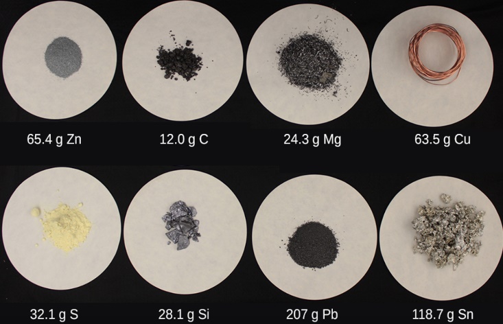
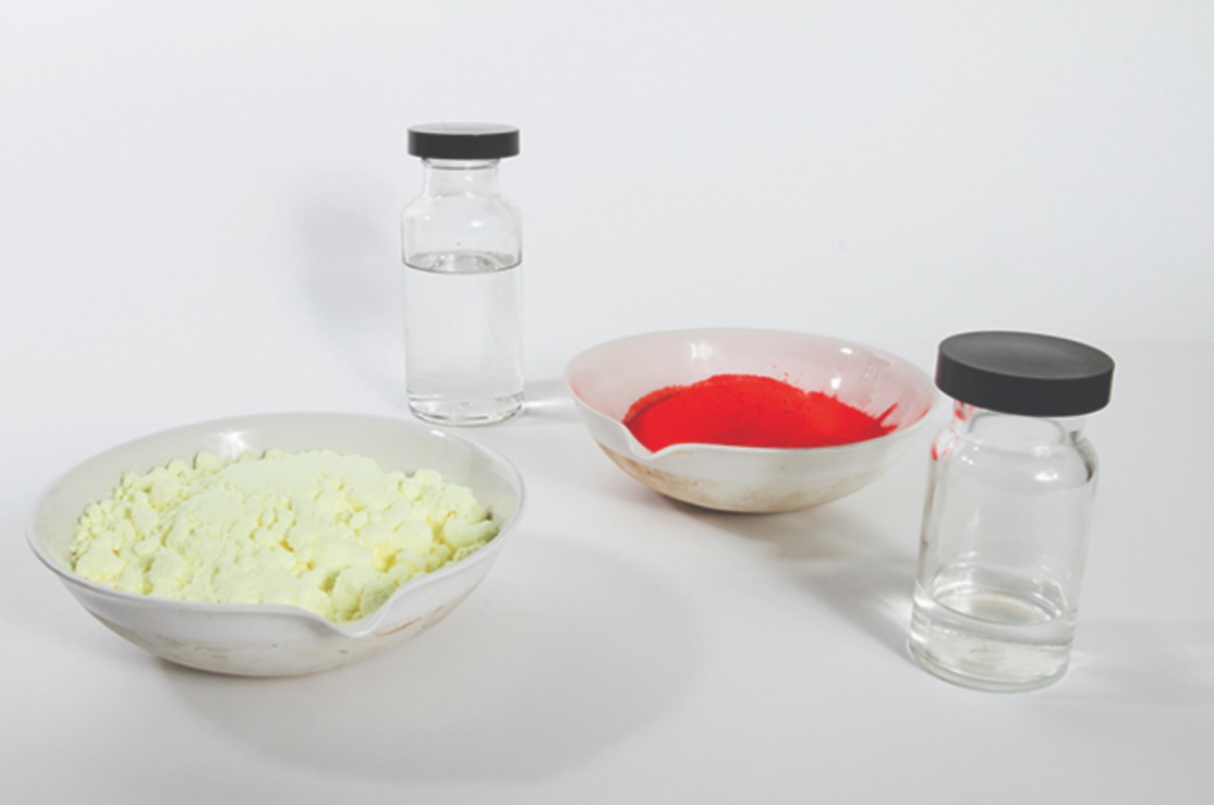
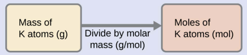
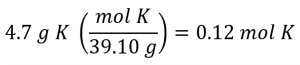
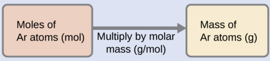
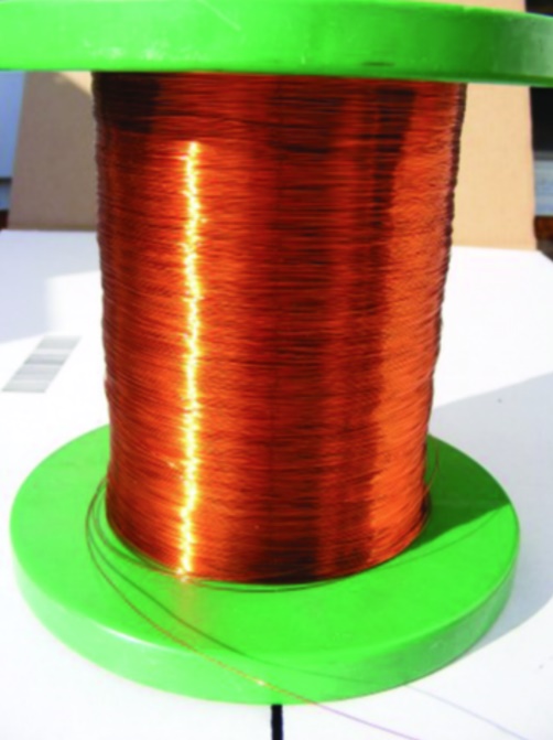
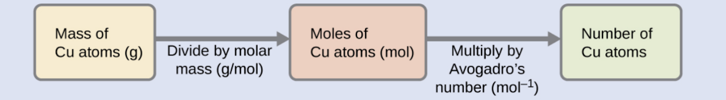
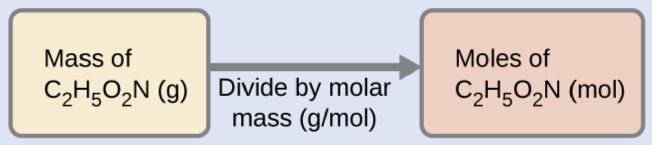
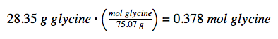 This result is consistent with our rough estimate.
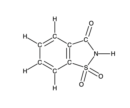
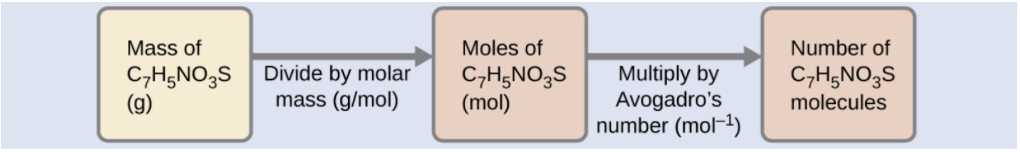
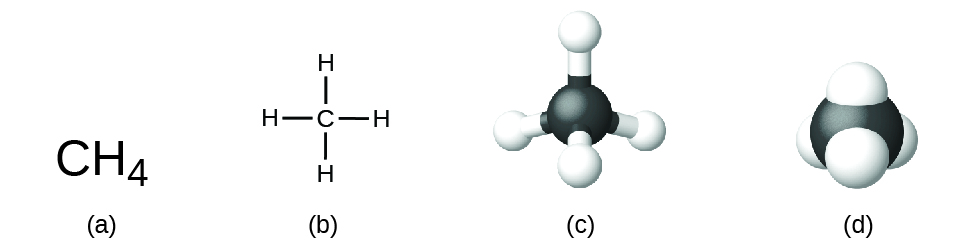
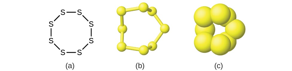
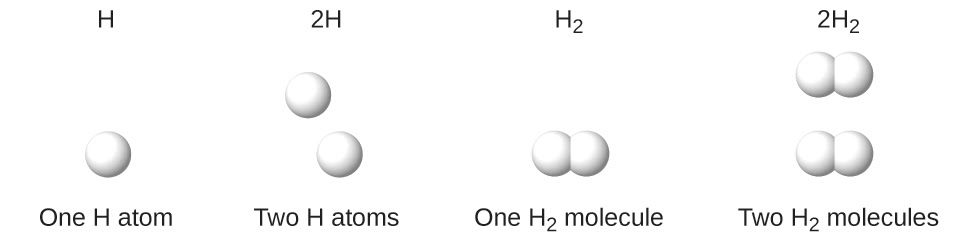
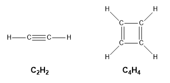
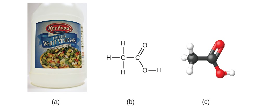
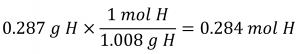
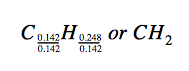
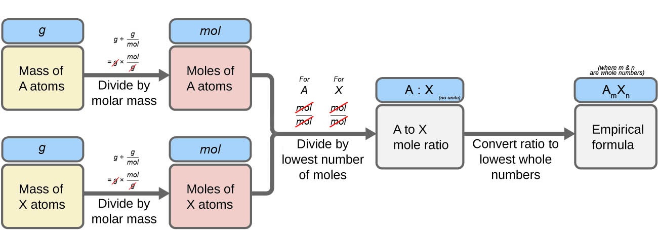
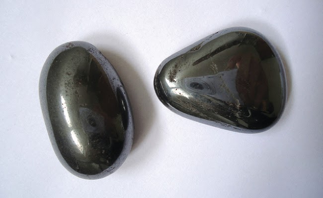
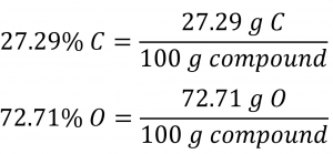
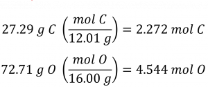
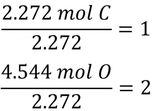
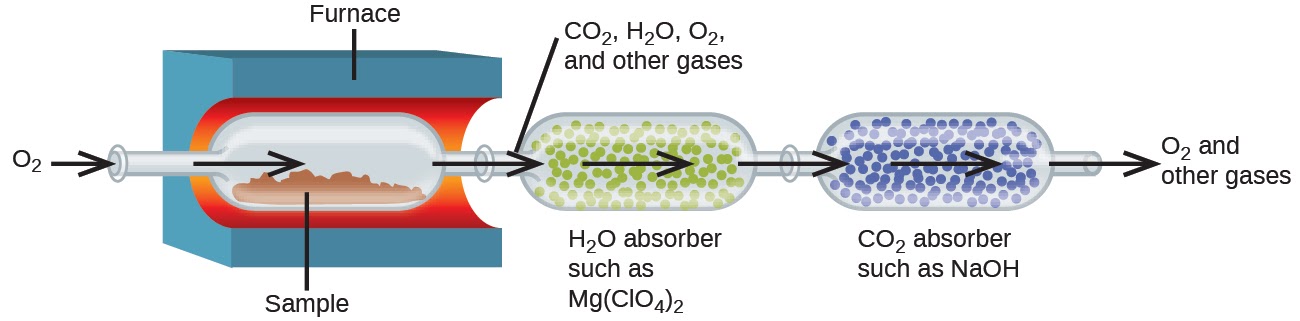
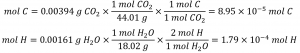
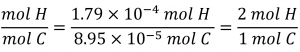
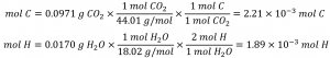
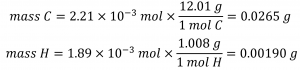
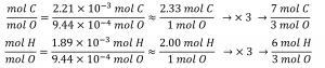
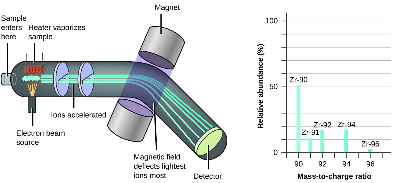
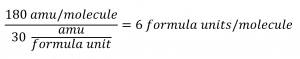
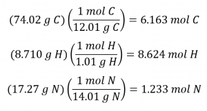
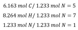
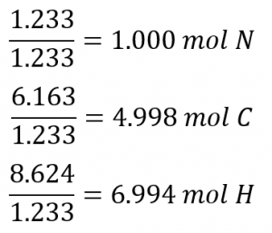
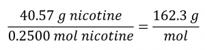
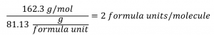
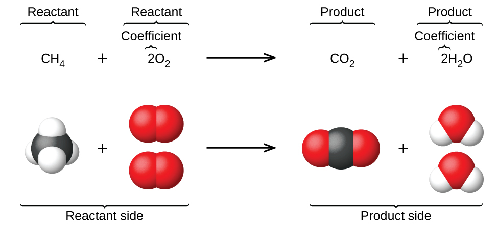
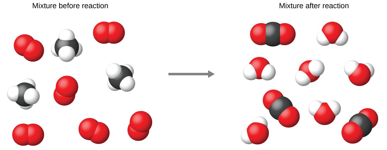
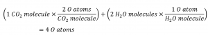
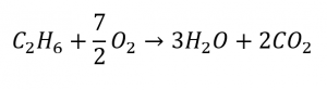
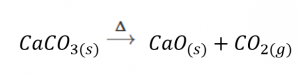

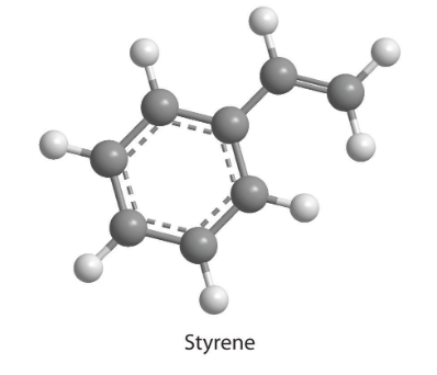
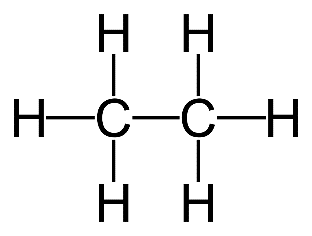
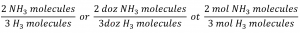
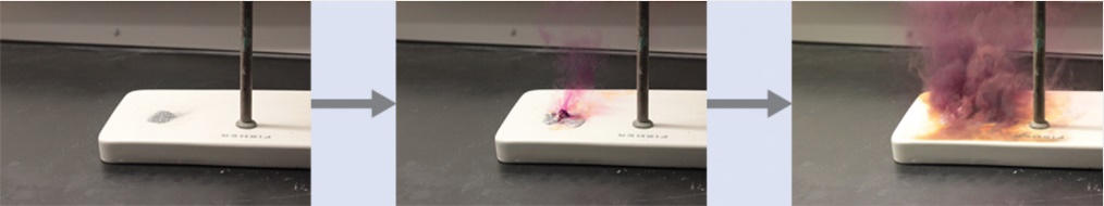
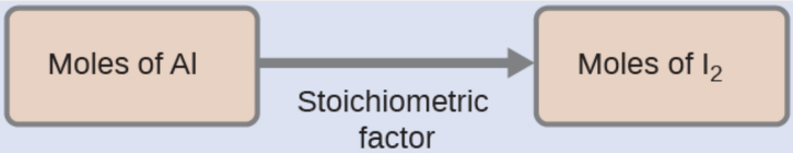
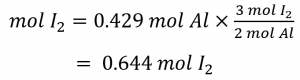
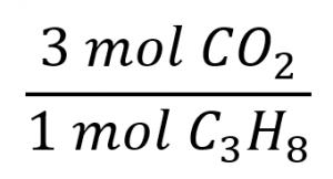
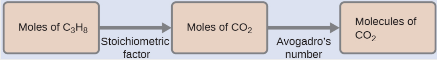
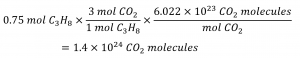
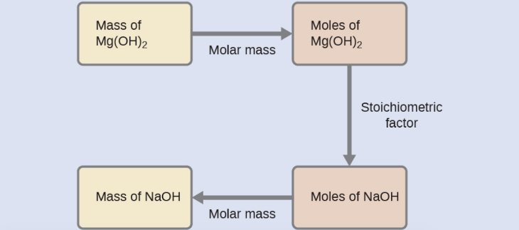
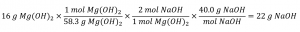
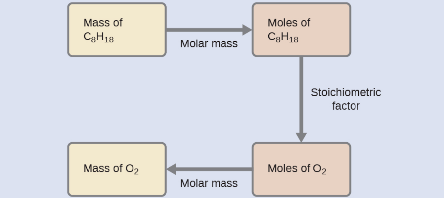
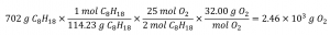
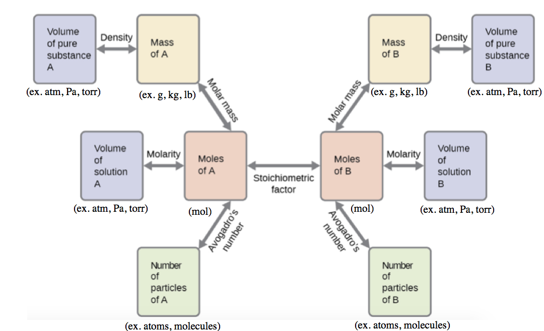
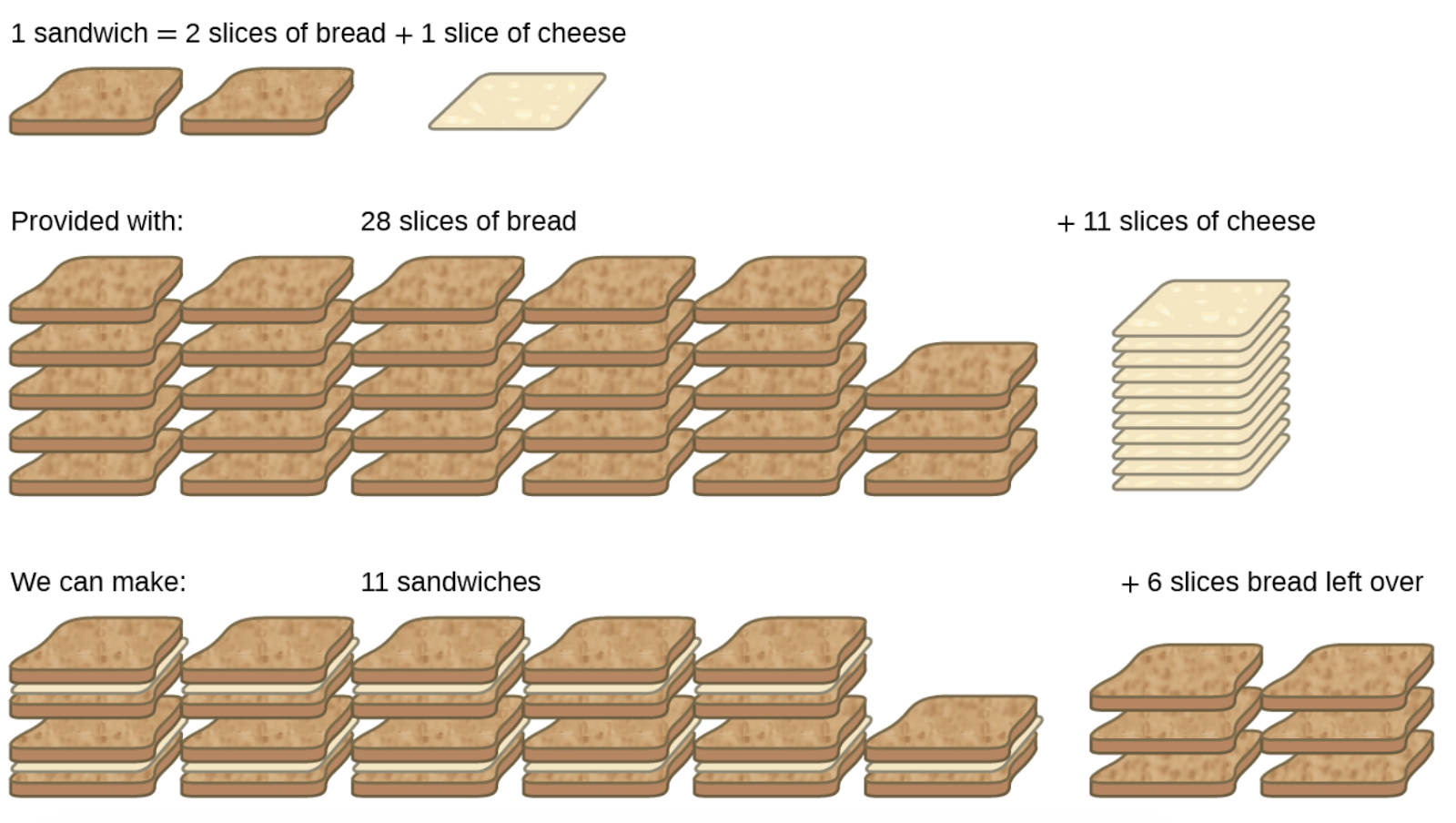
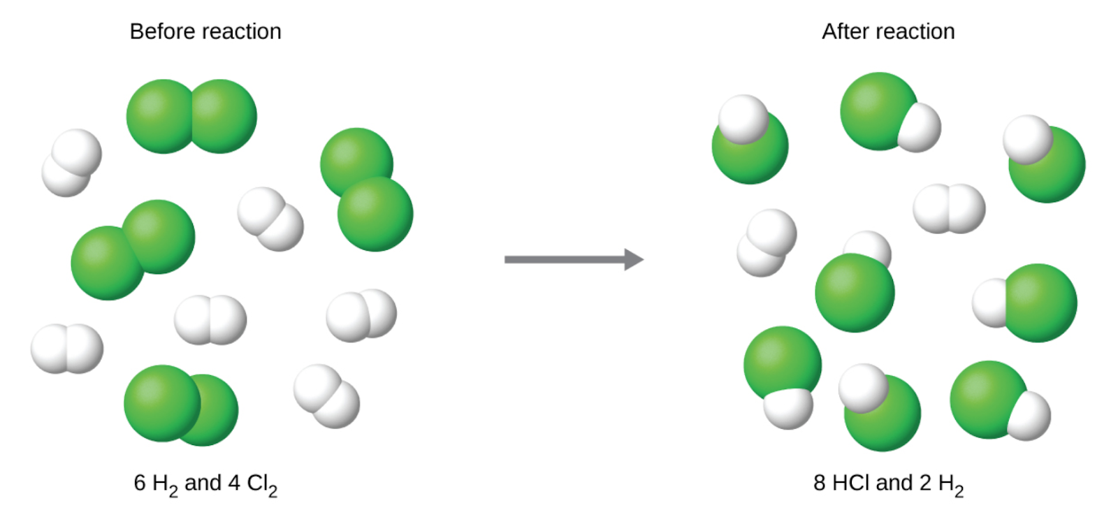
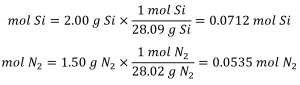
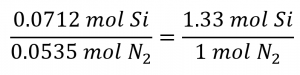
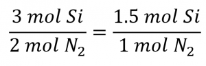


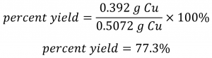
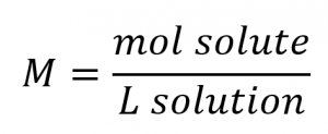
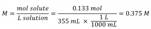
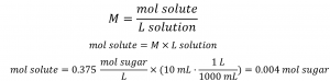
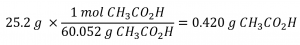
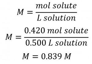
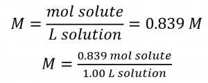
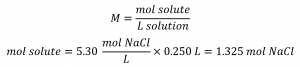
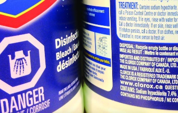
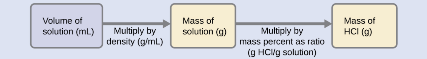
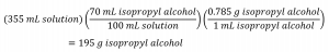
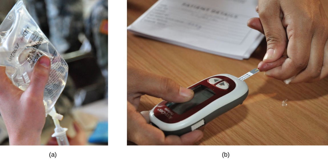
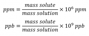
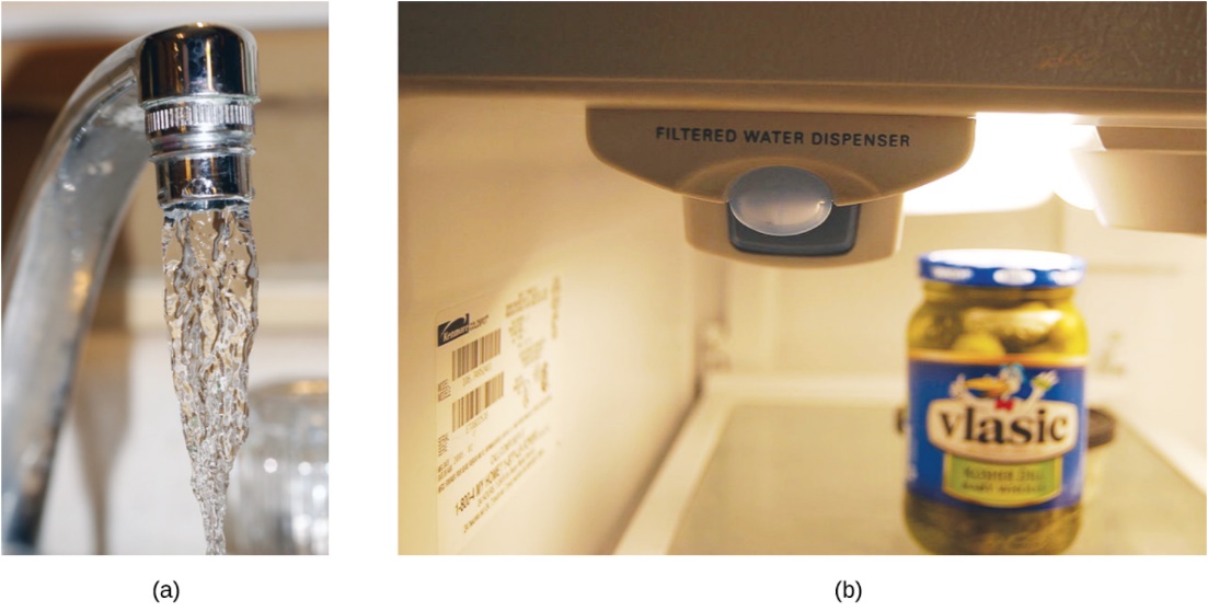
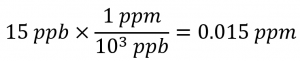
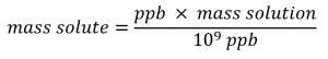
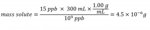
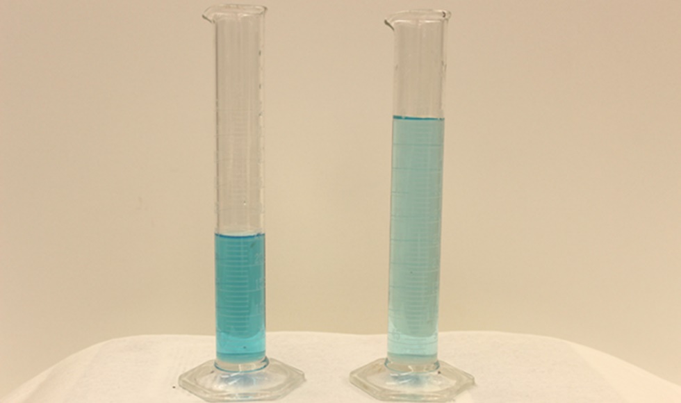
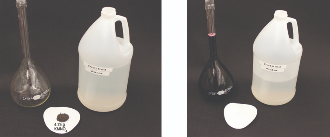
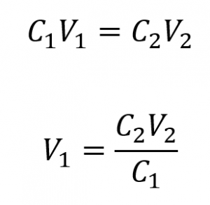
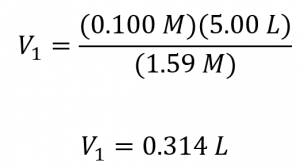
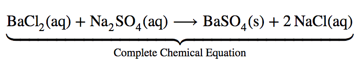
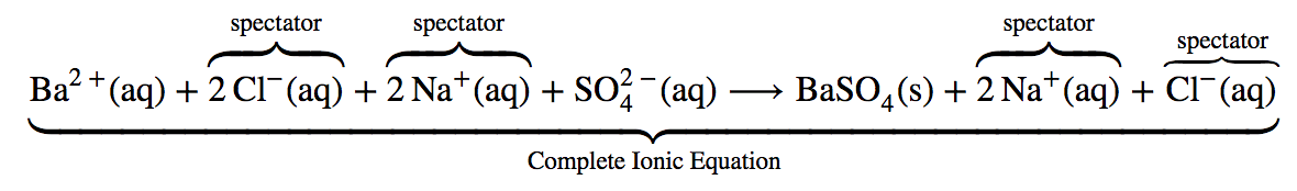
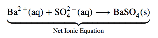
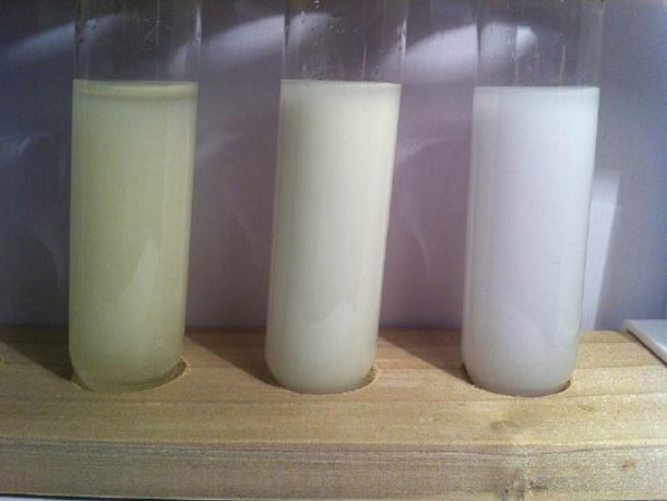

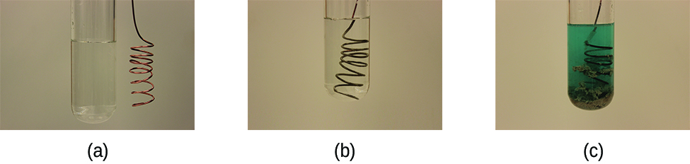
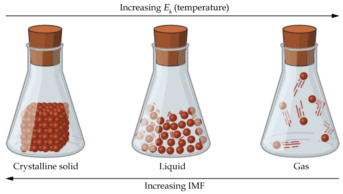
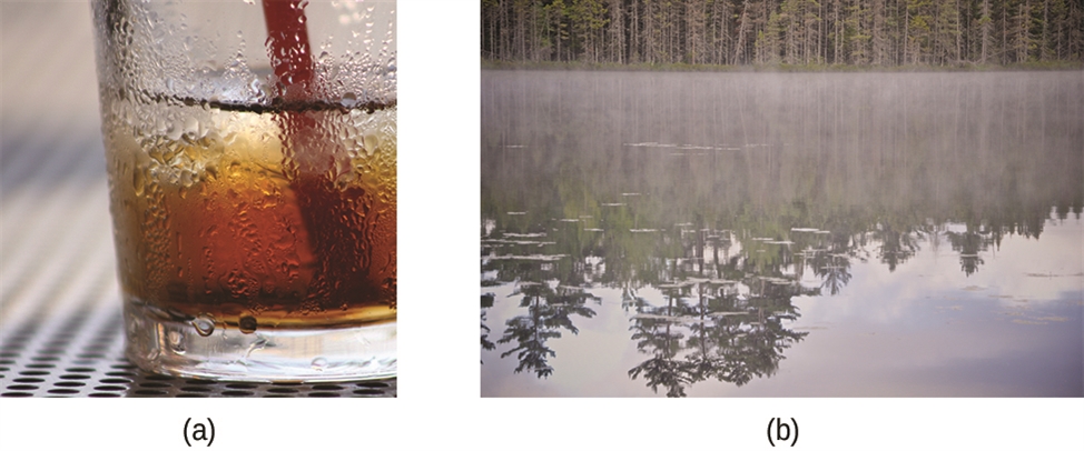
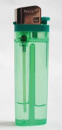
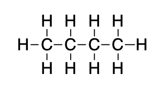
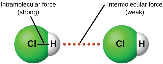
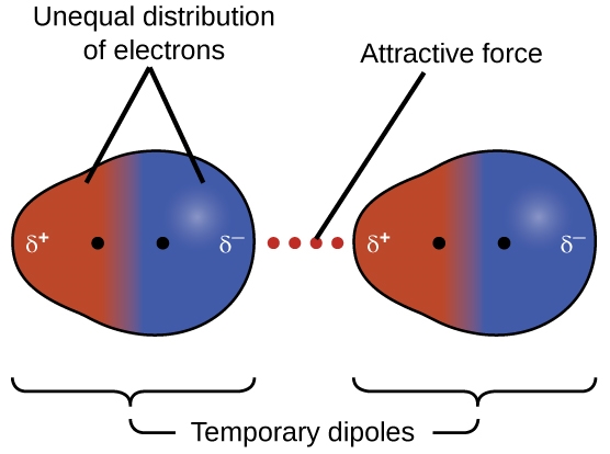
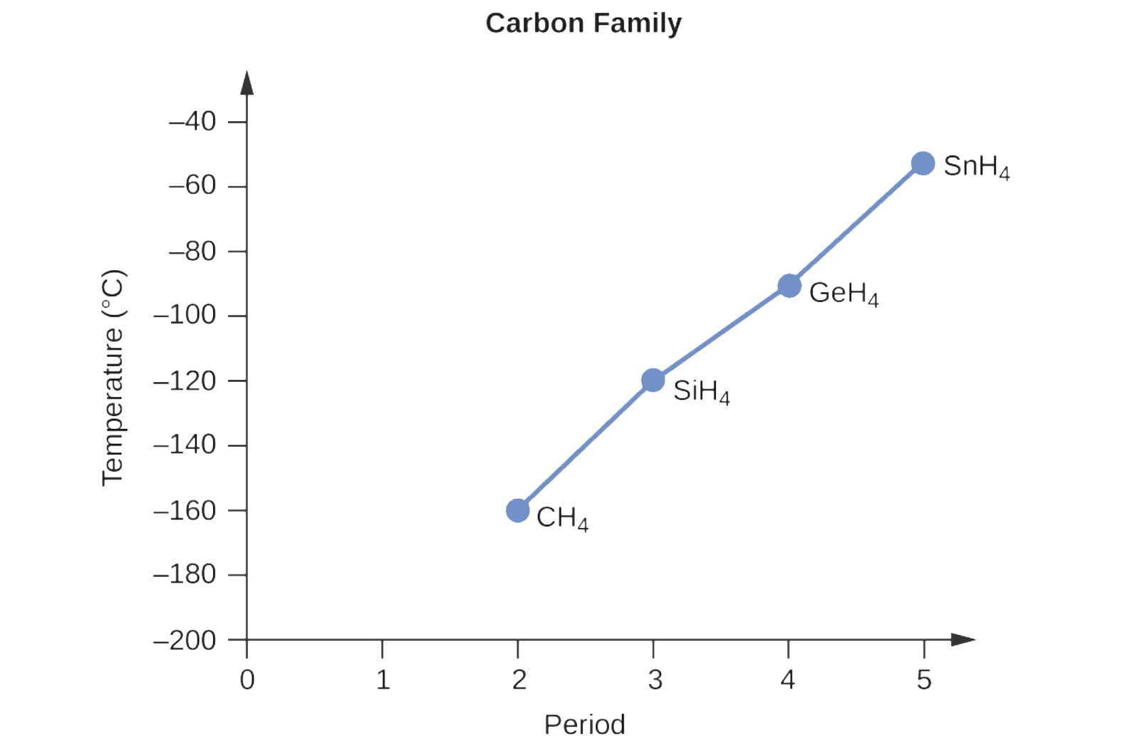
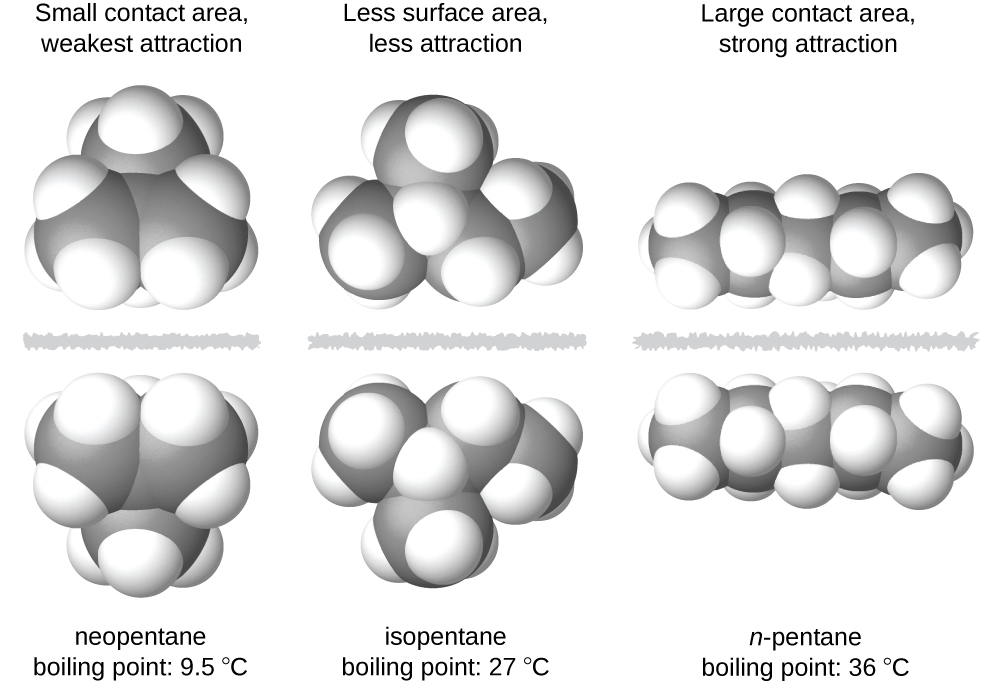
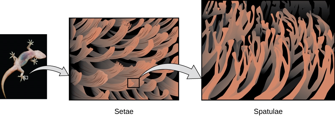
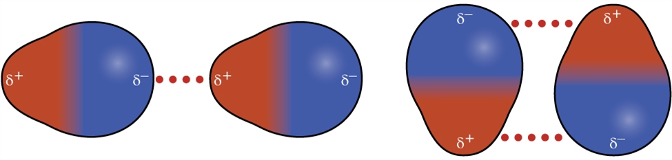
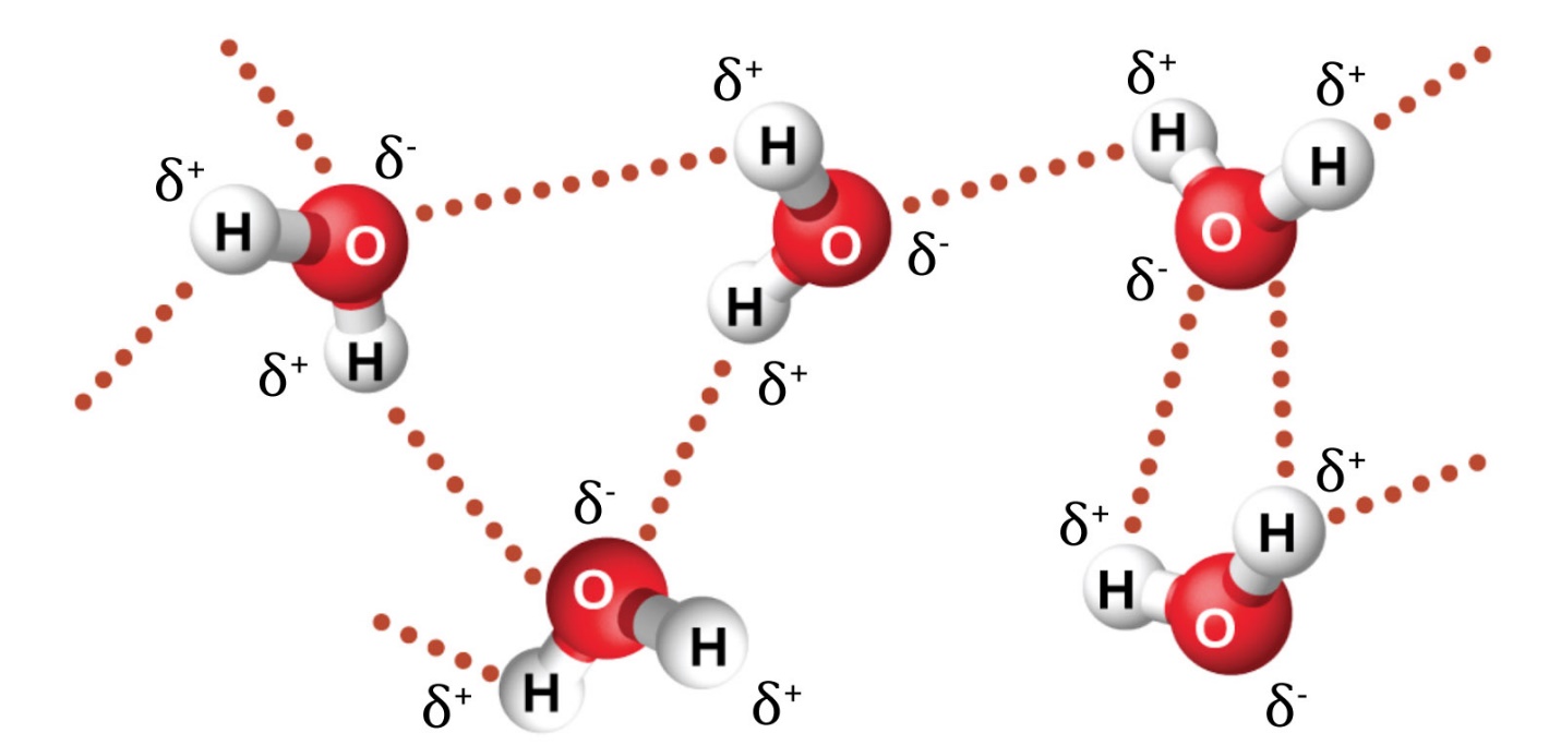
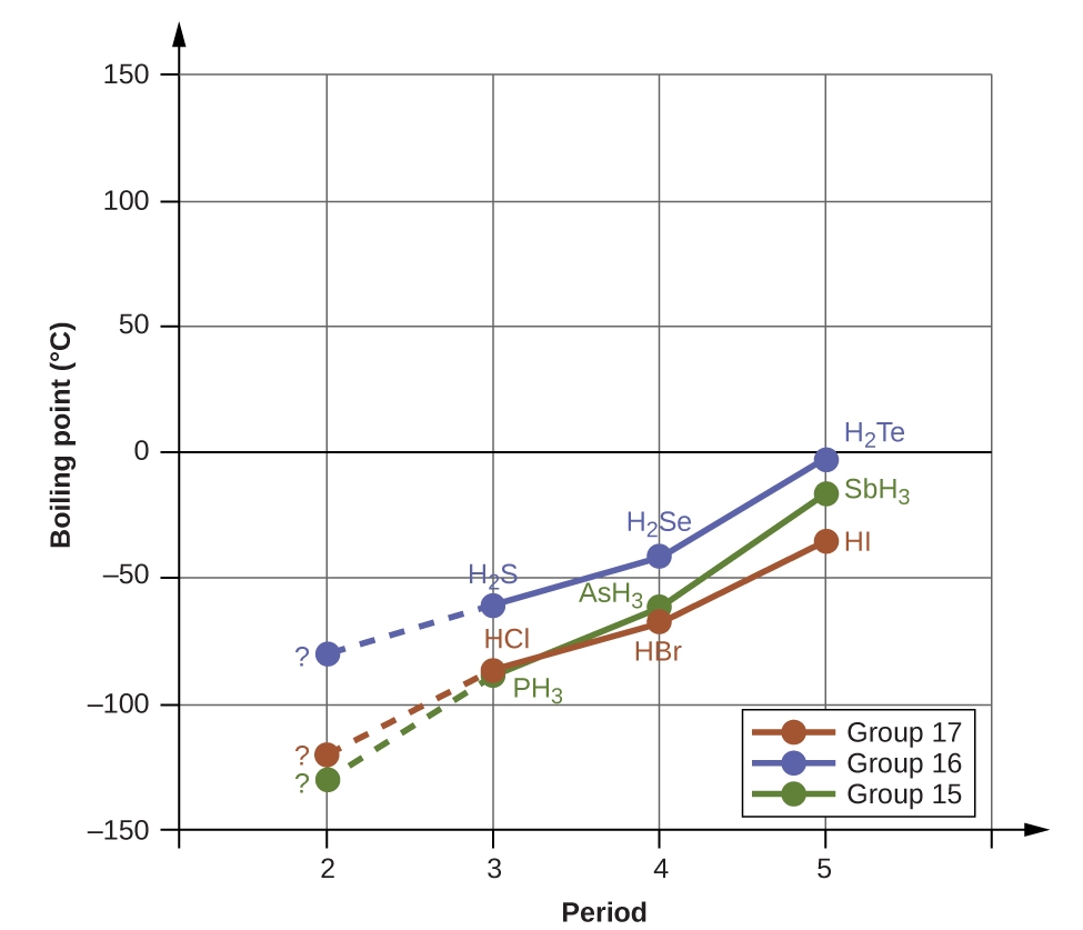
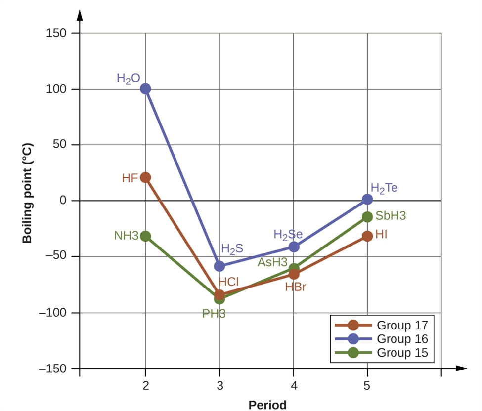
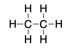
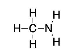
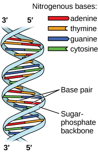
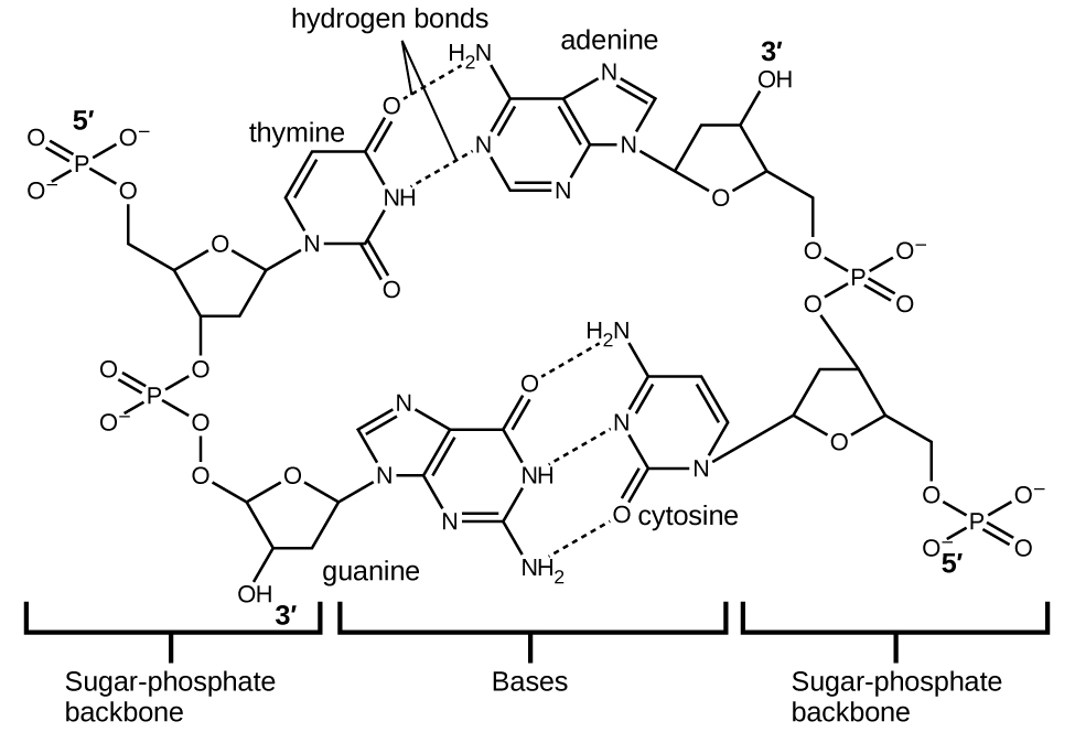
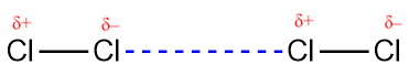
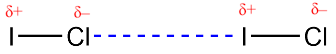
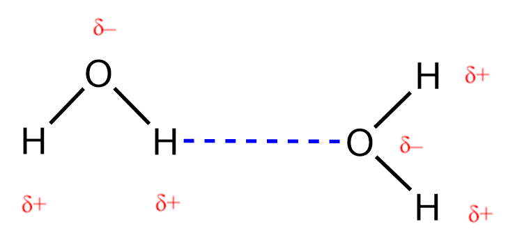
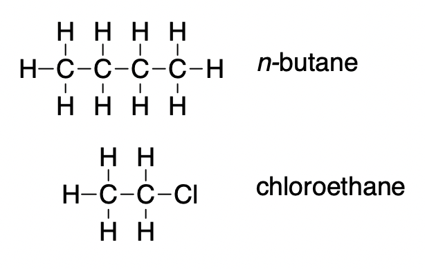
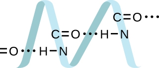
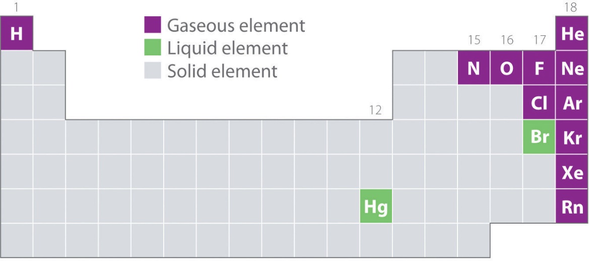
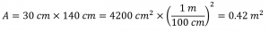
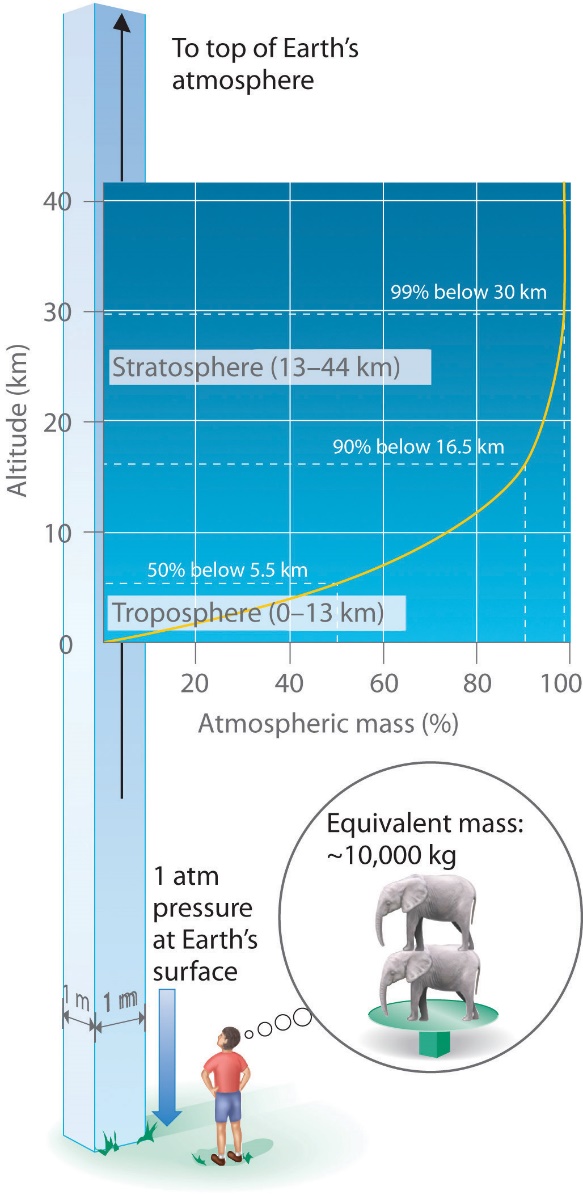
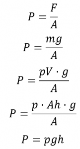
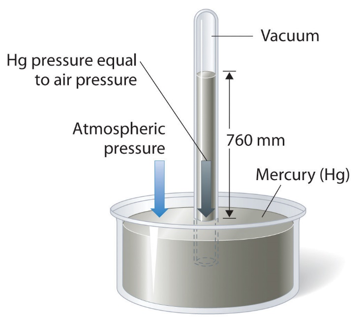
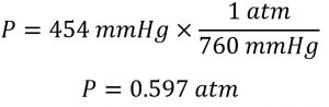
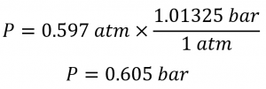
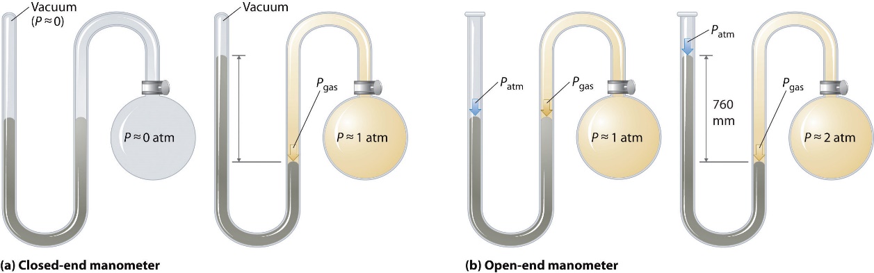
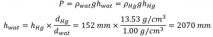
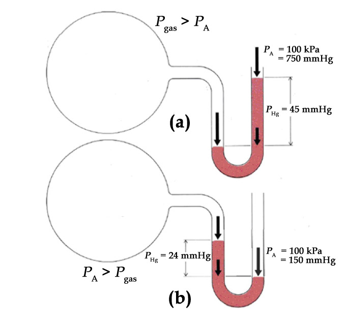
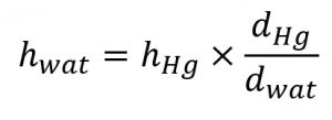
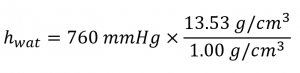
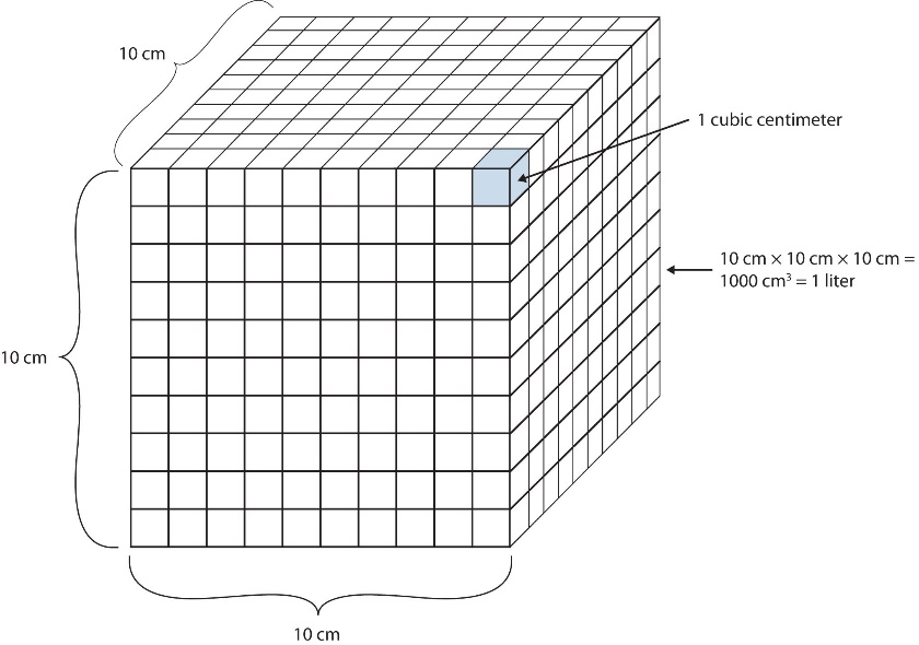
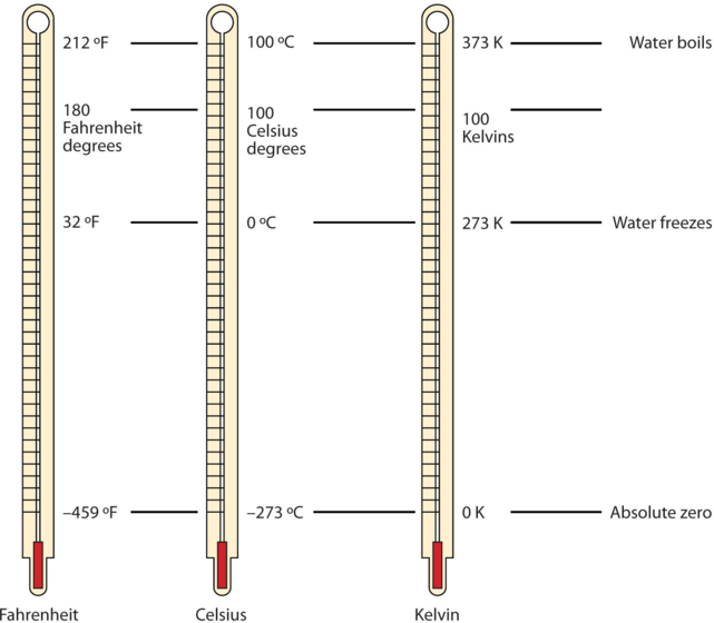
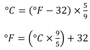
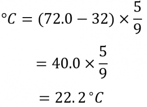
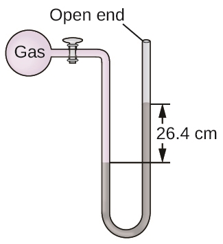
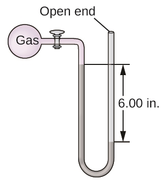
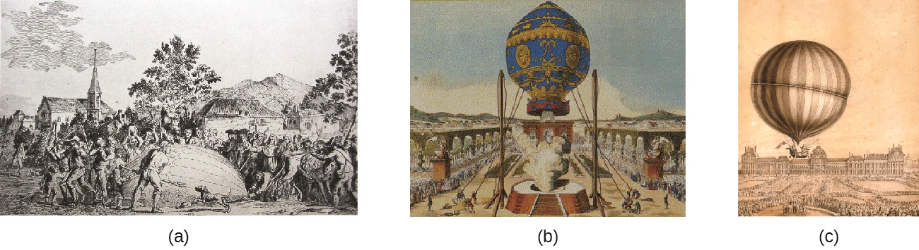
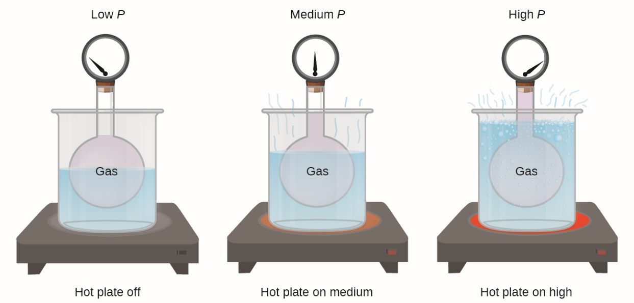
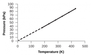
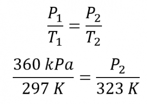
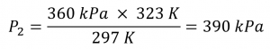
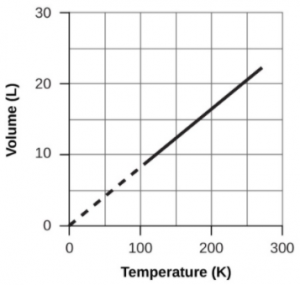
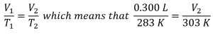
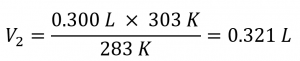
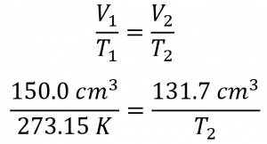
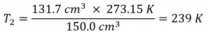
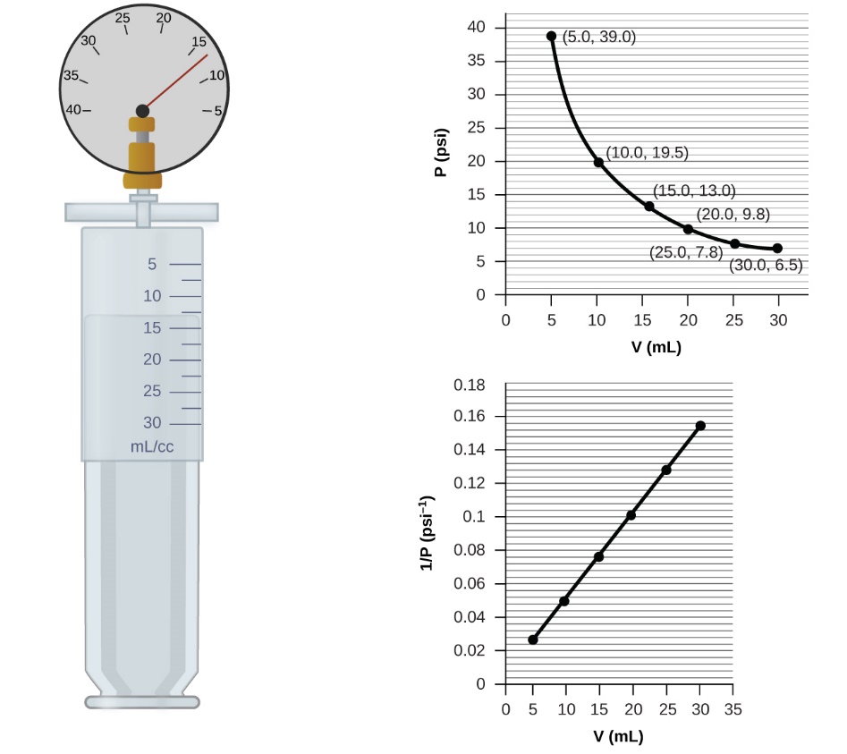
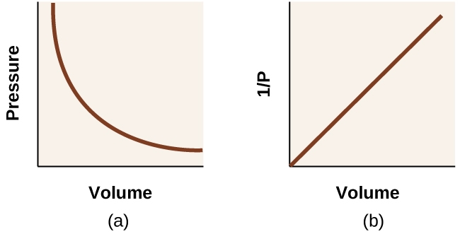
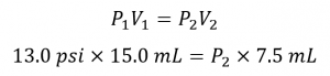
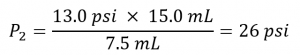
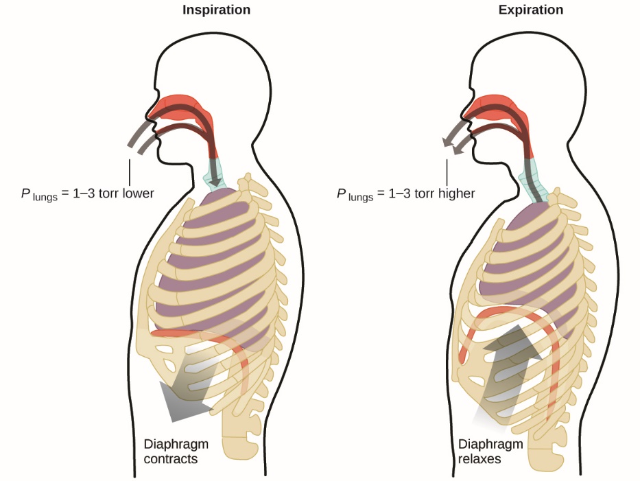
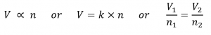
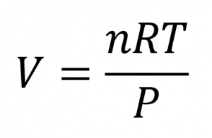
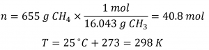

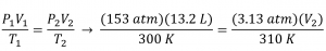
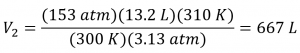
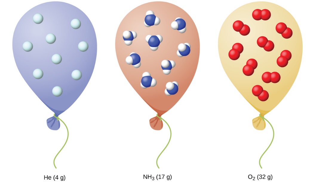

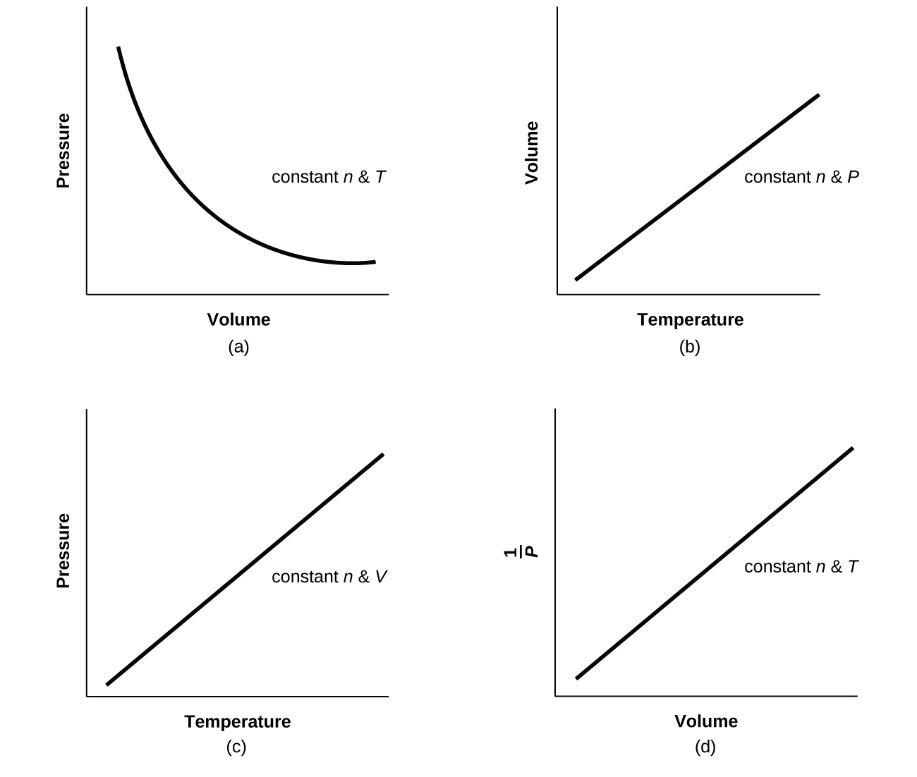
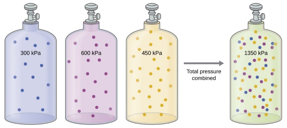
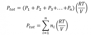
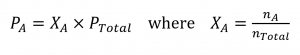
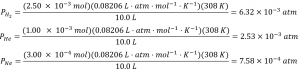
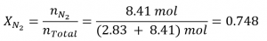
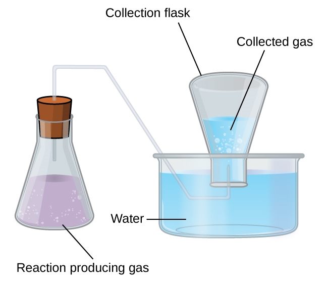
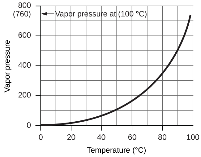
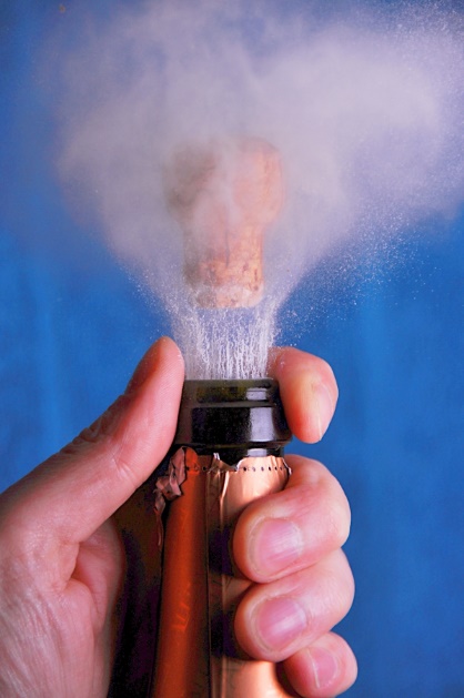
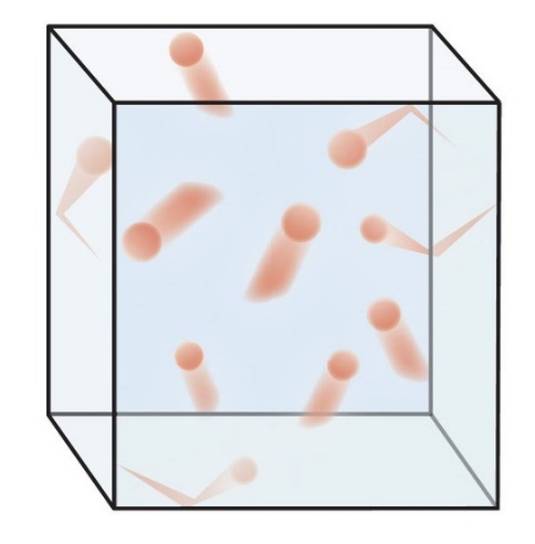
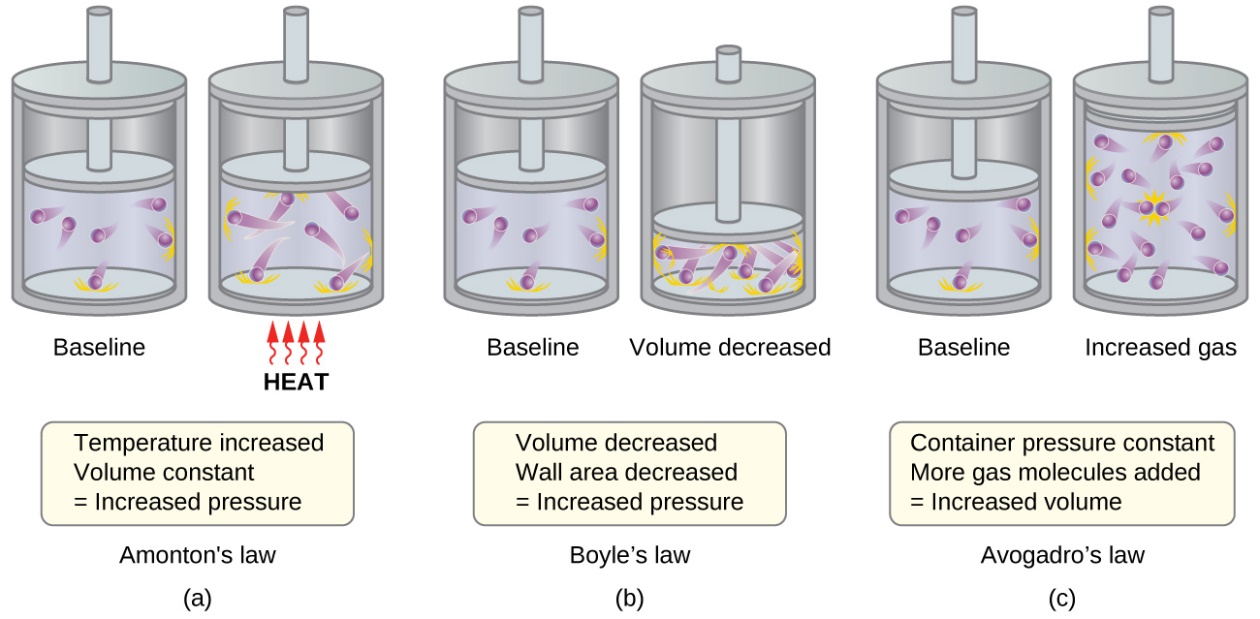
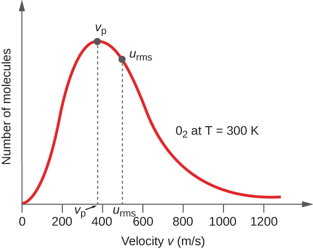
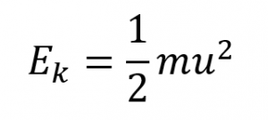
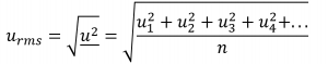
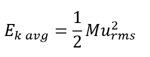
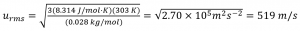
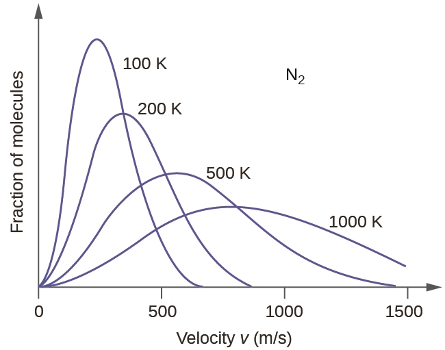
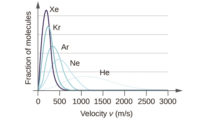
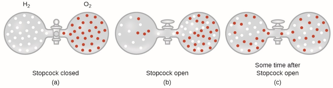
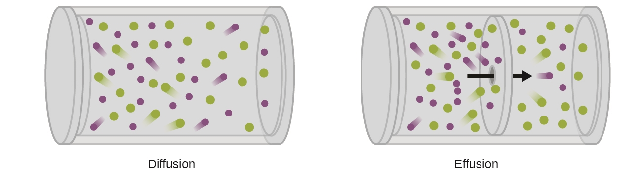
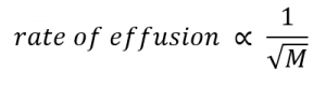
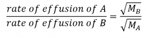
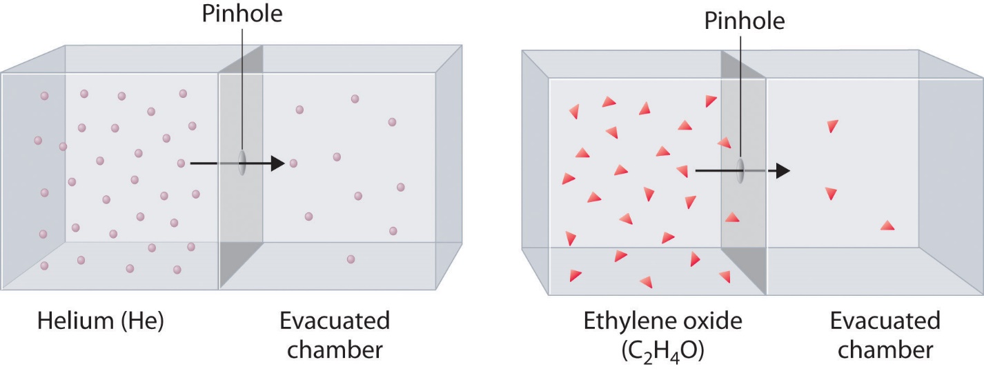
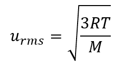
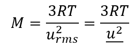
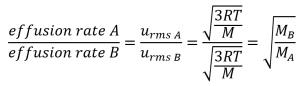
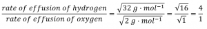
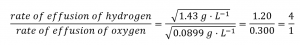
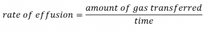
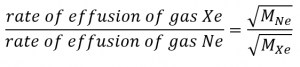
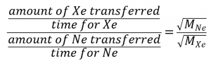
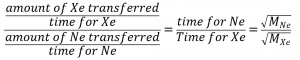
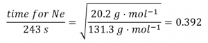

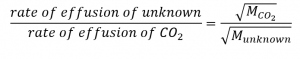
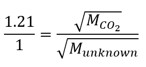
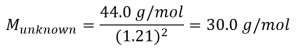
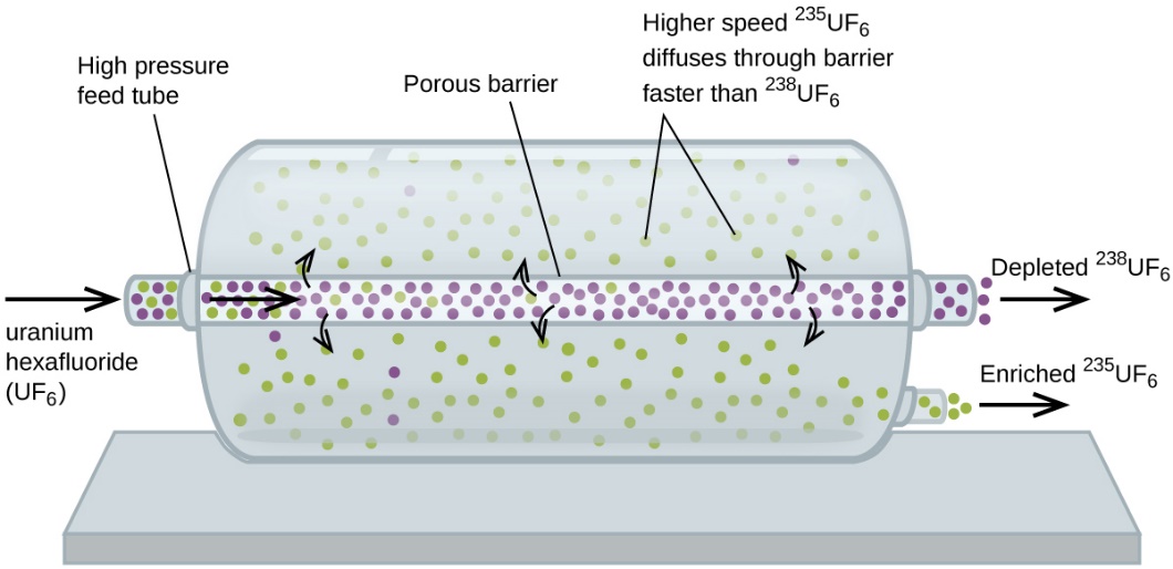
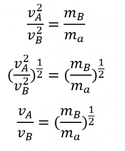
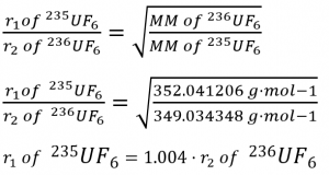
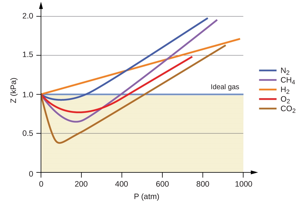
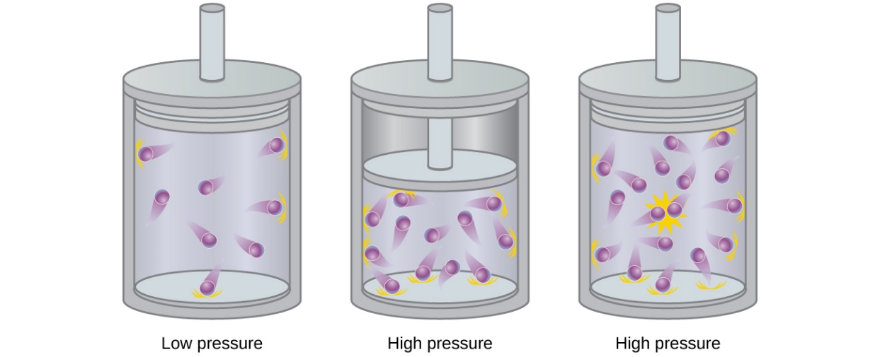
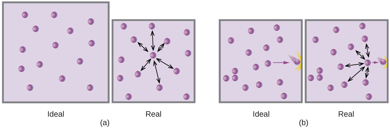
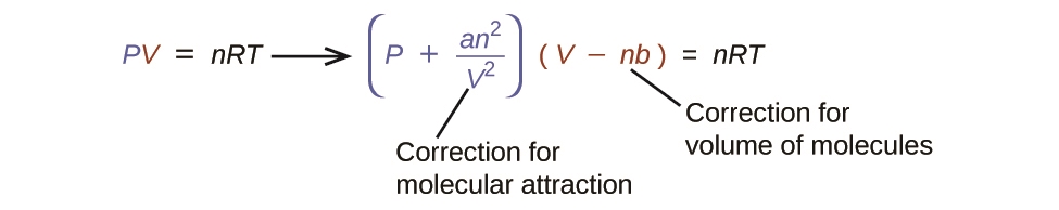
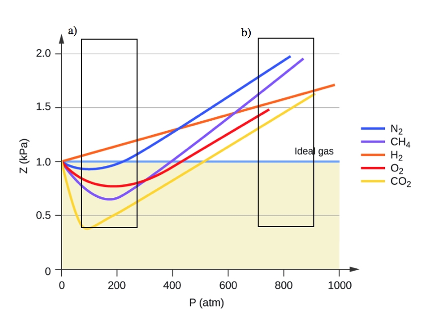
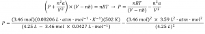
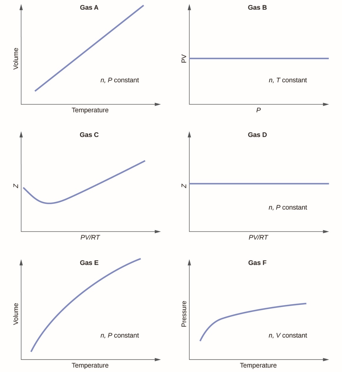
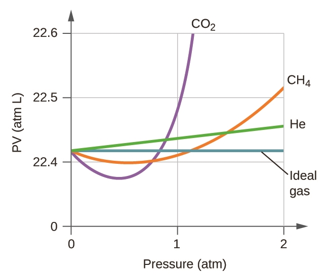
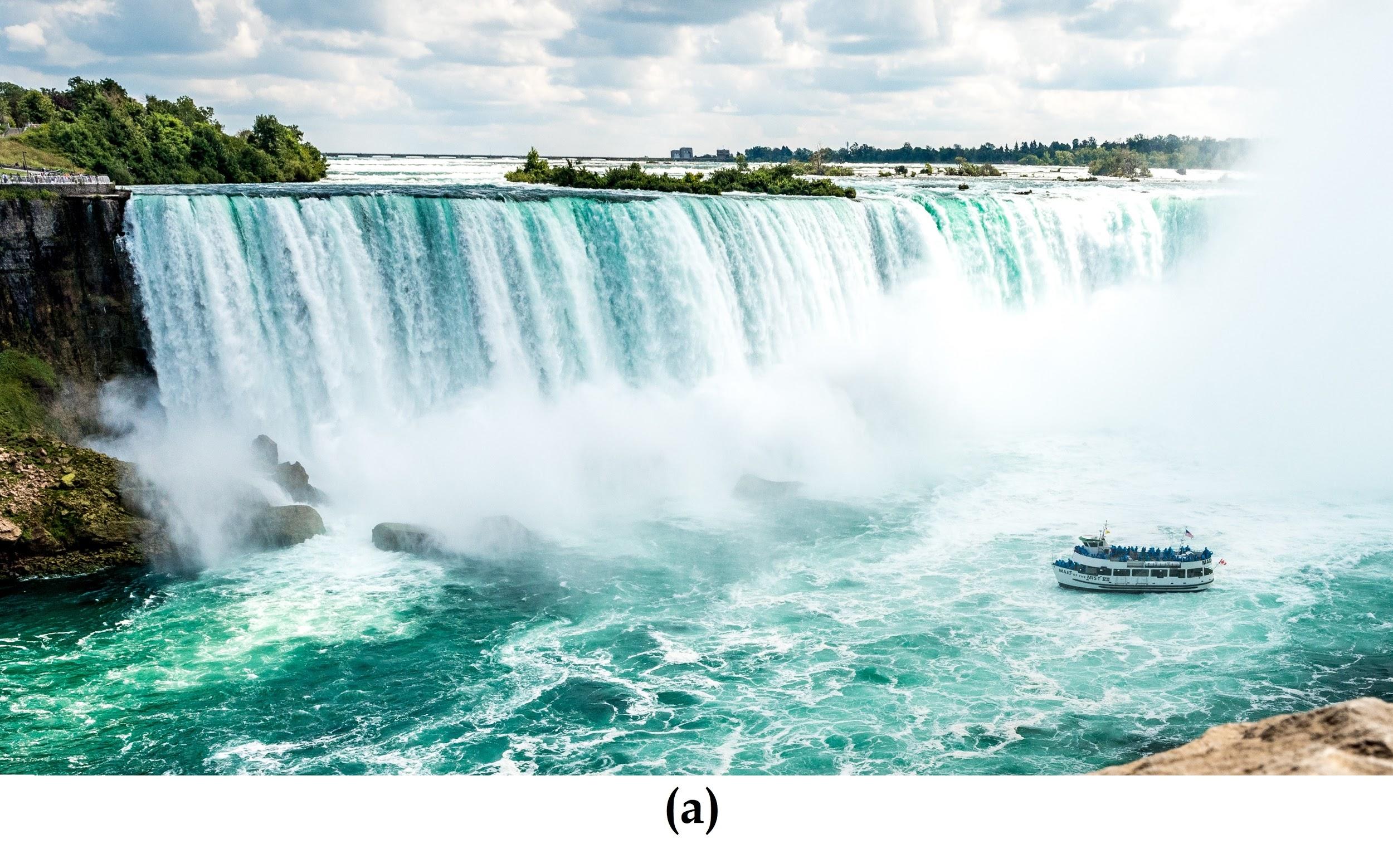
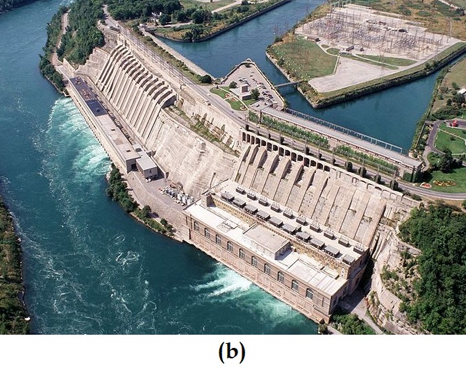
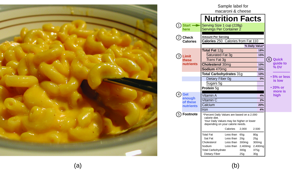
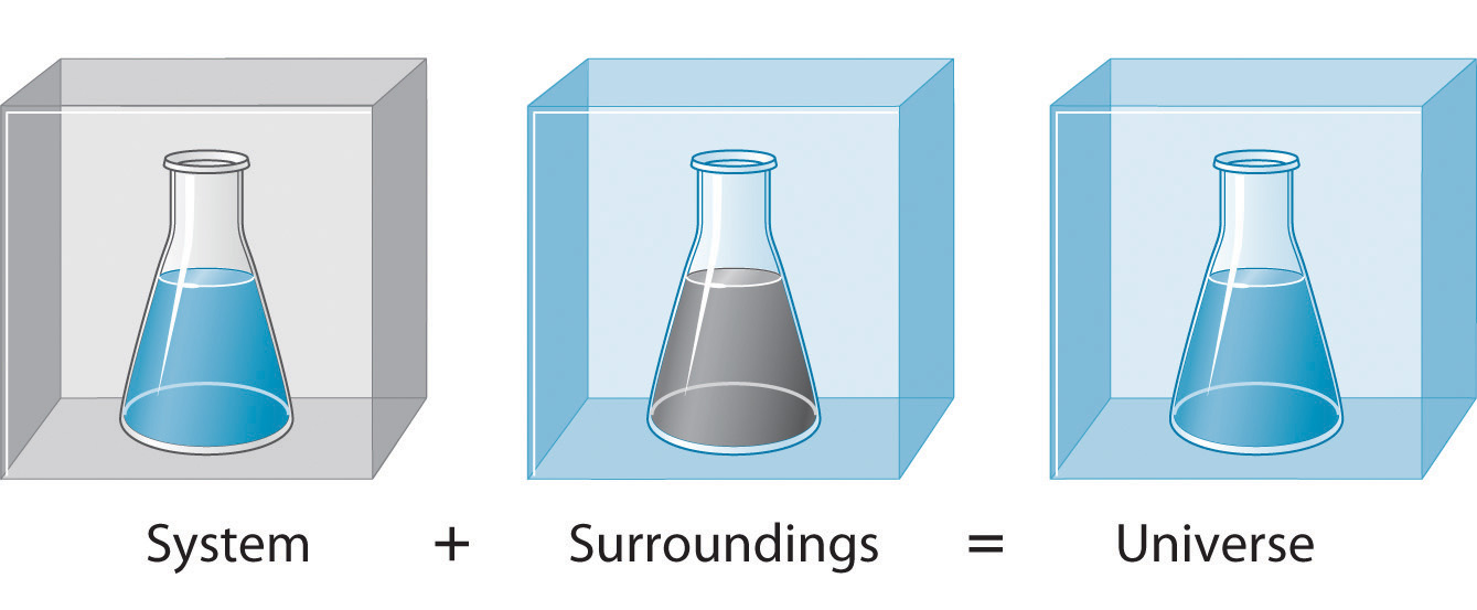
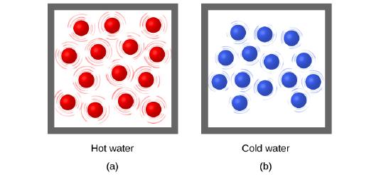
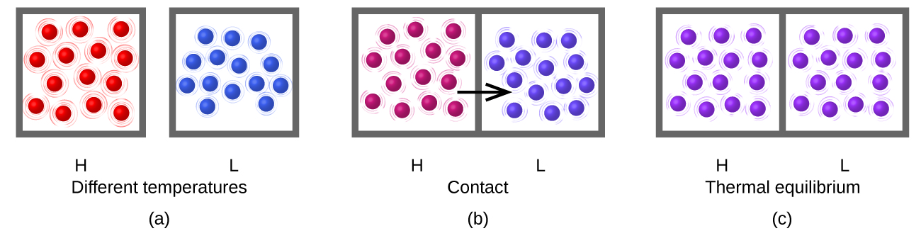
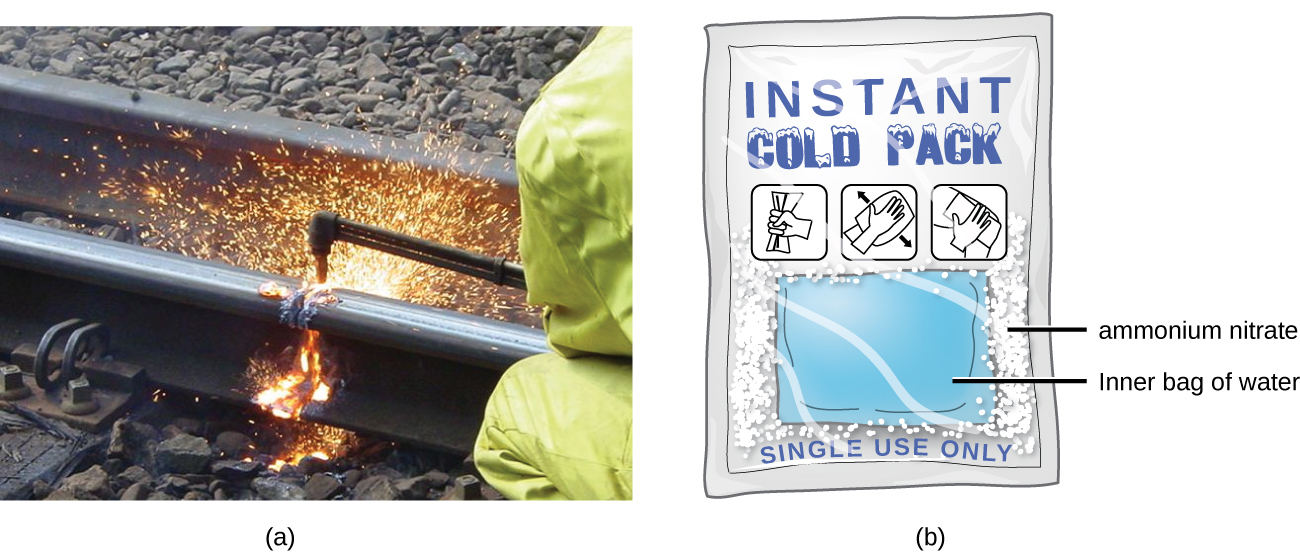
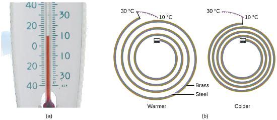
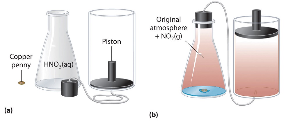
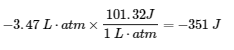
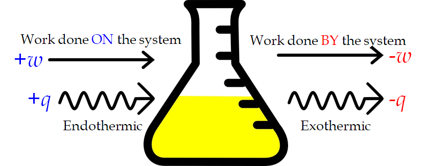
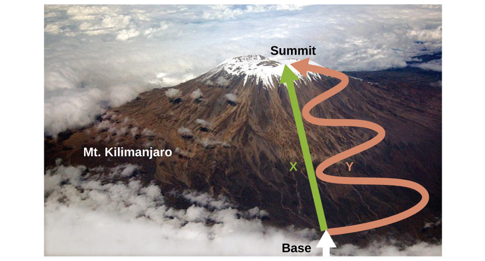
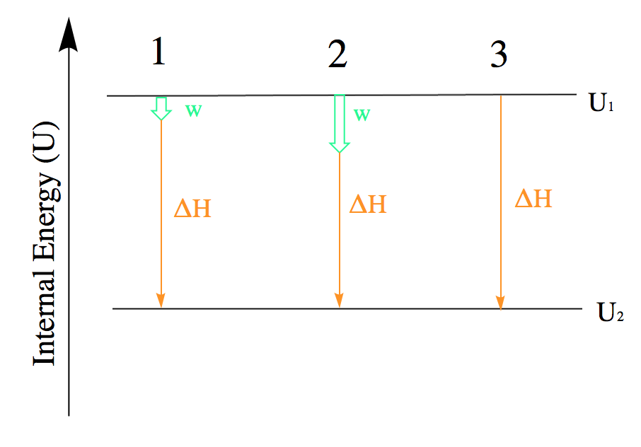
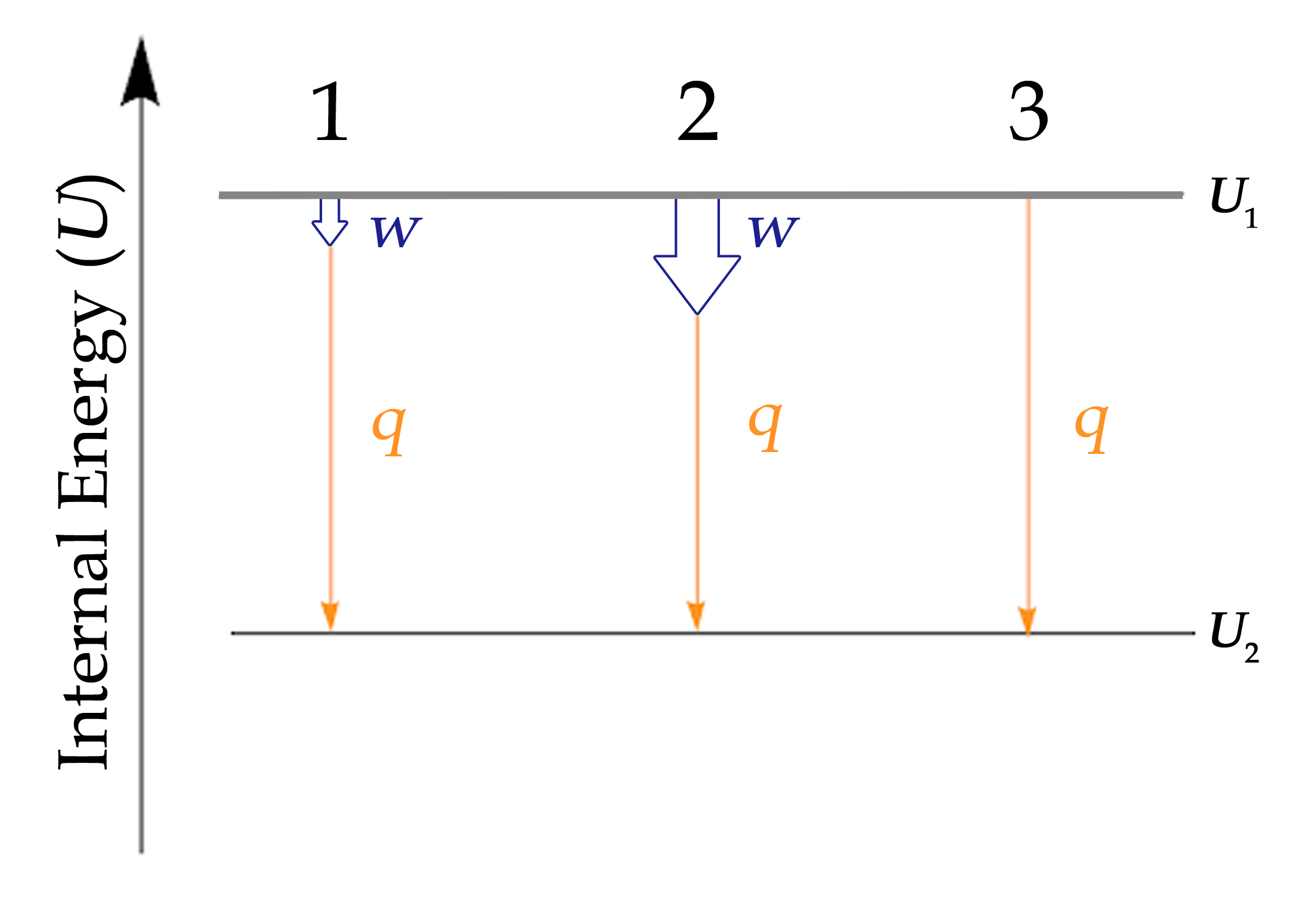
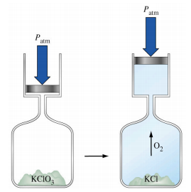
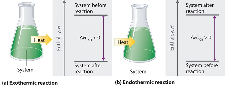
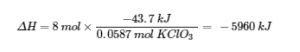
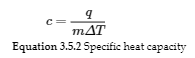
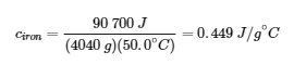

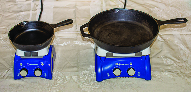
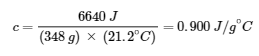
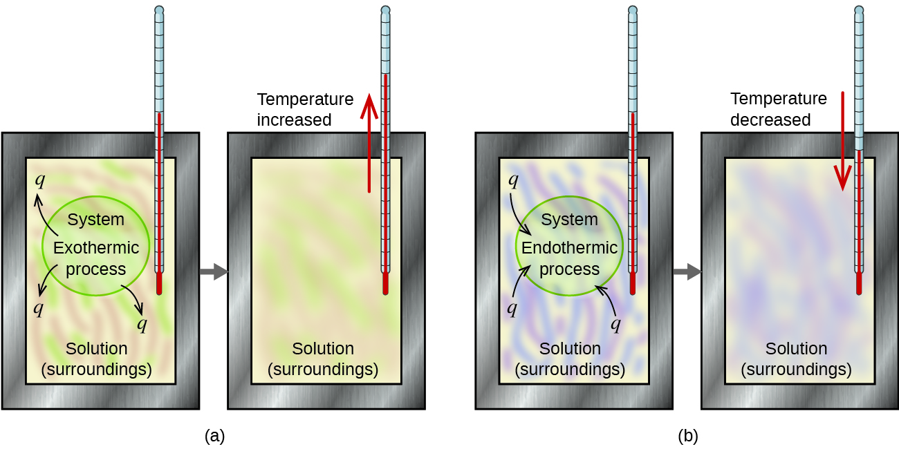
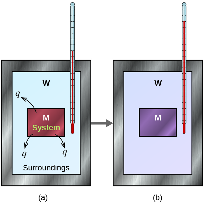
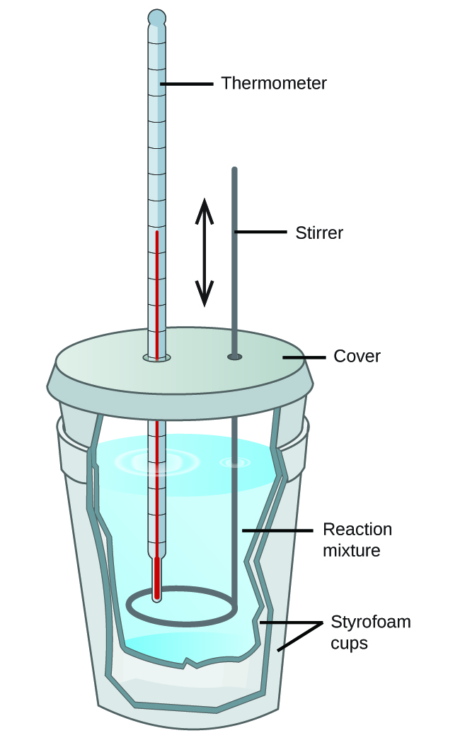
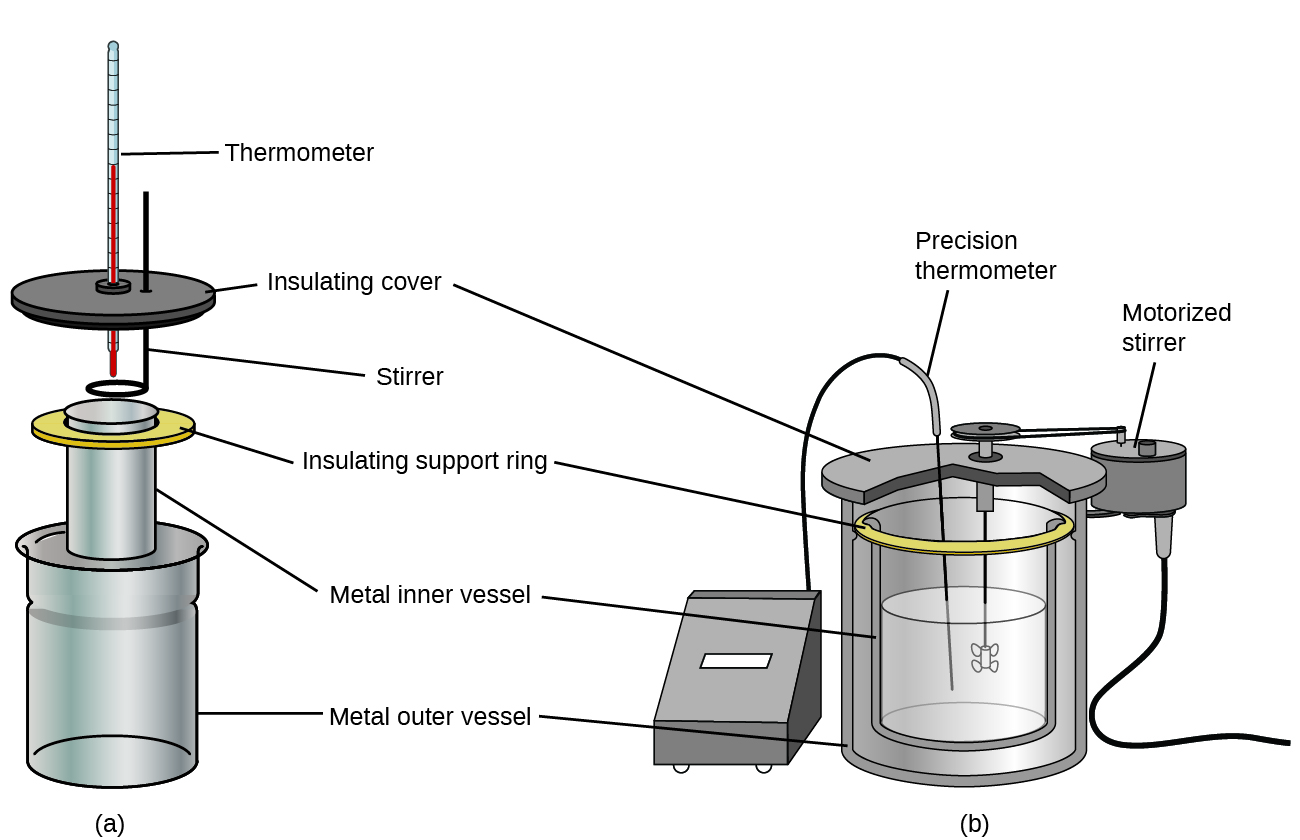
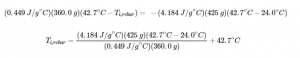 Solving this gives Ti,rebar= 248°C, so the initial temperature of the rebar was 248°C.
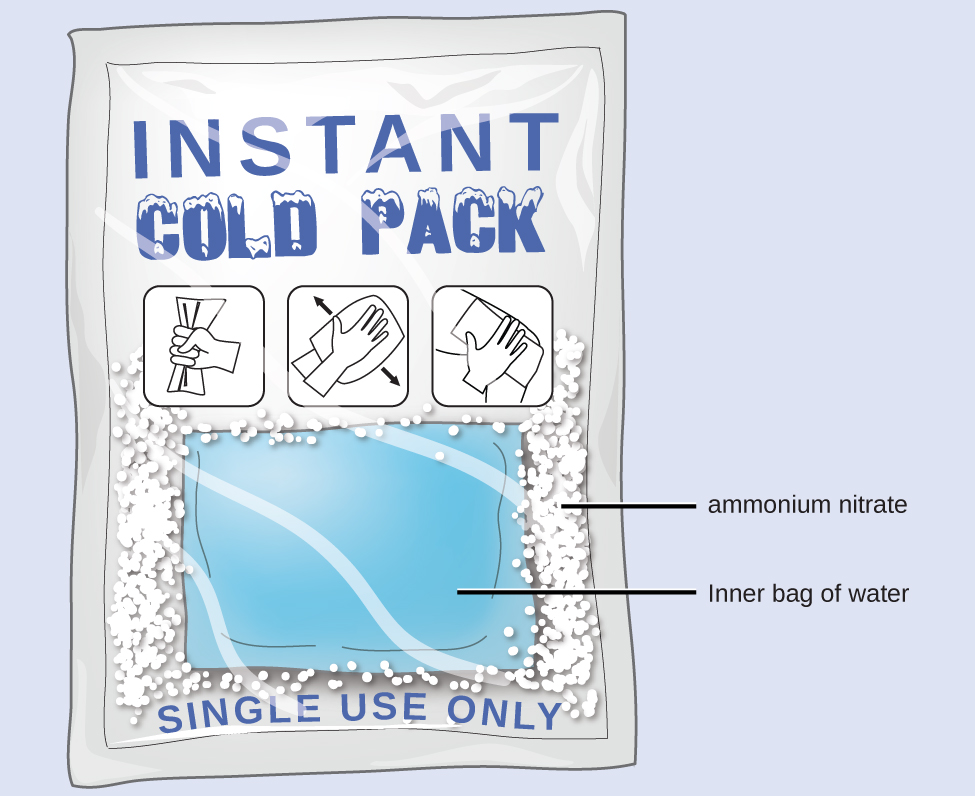
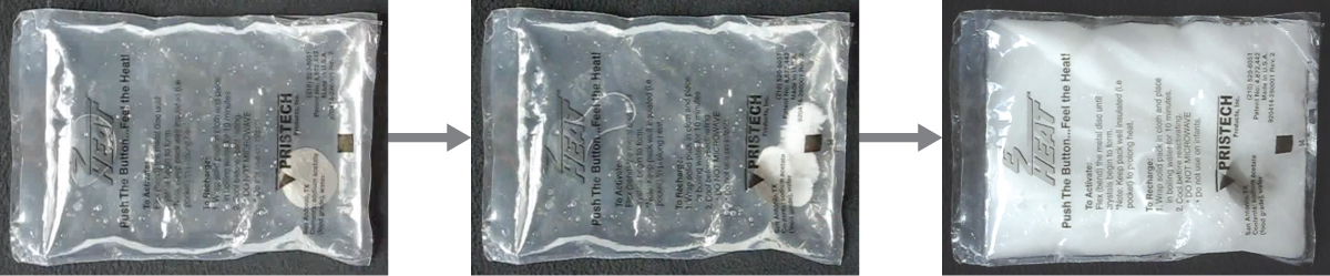
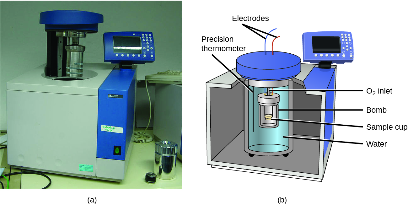
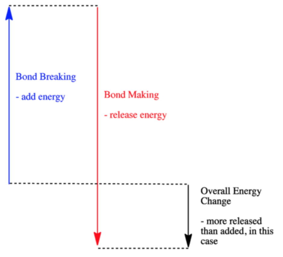
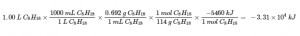
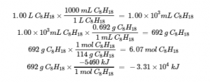
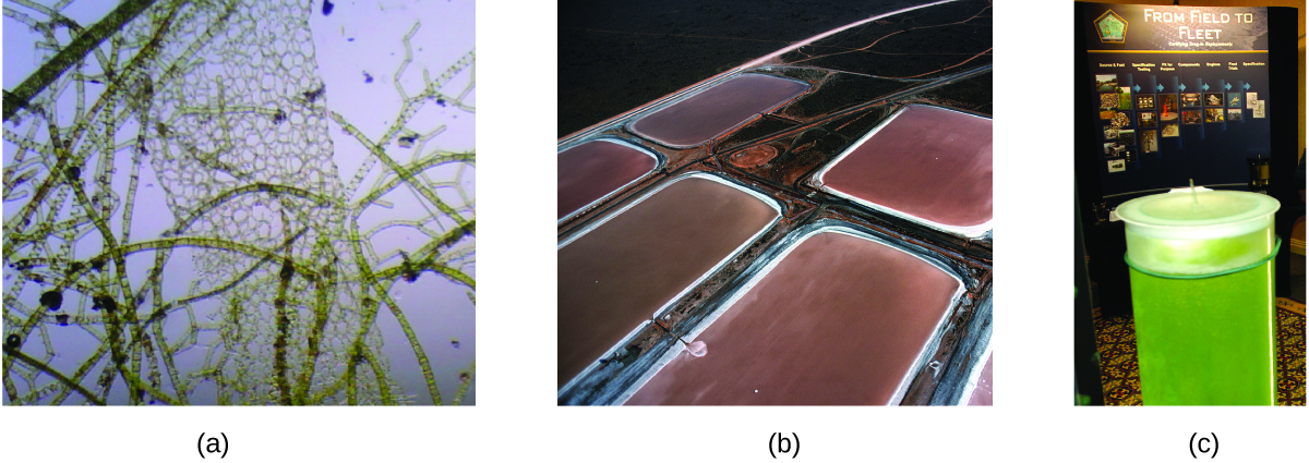
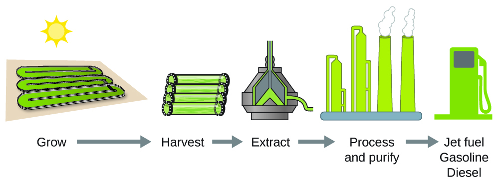
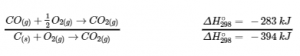
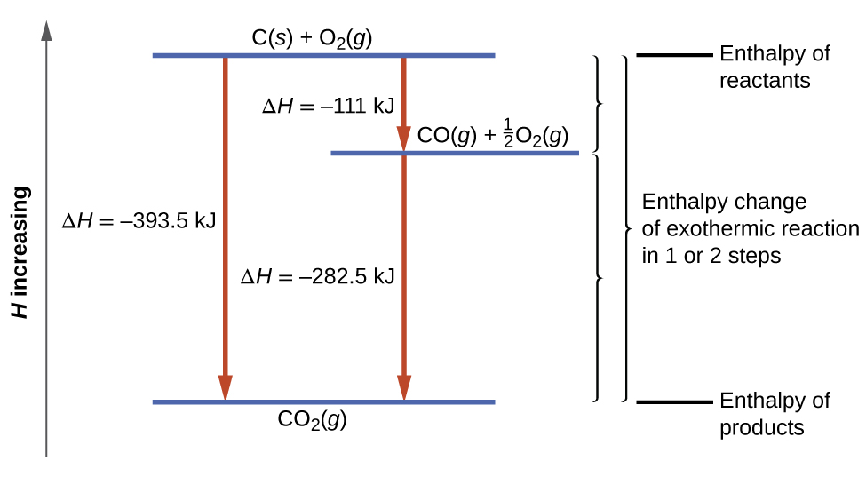
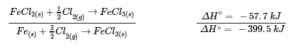
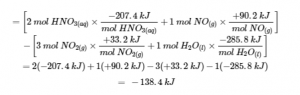
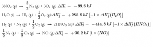
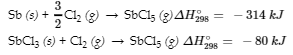
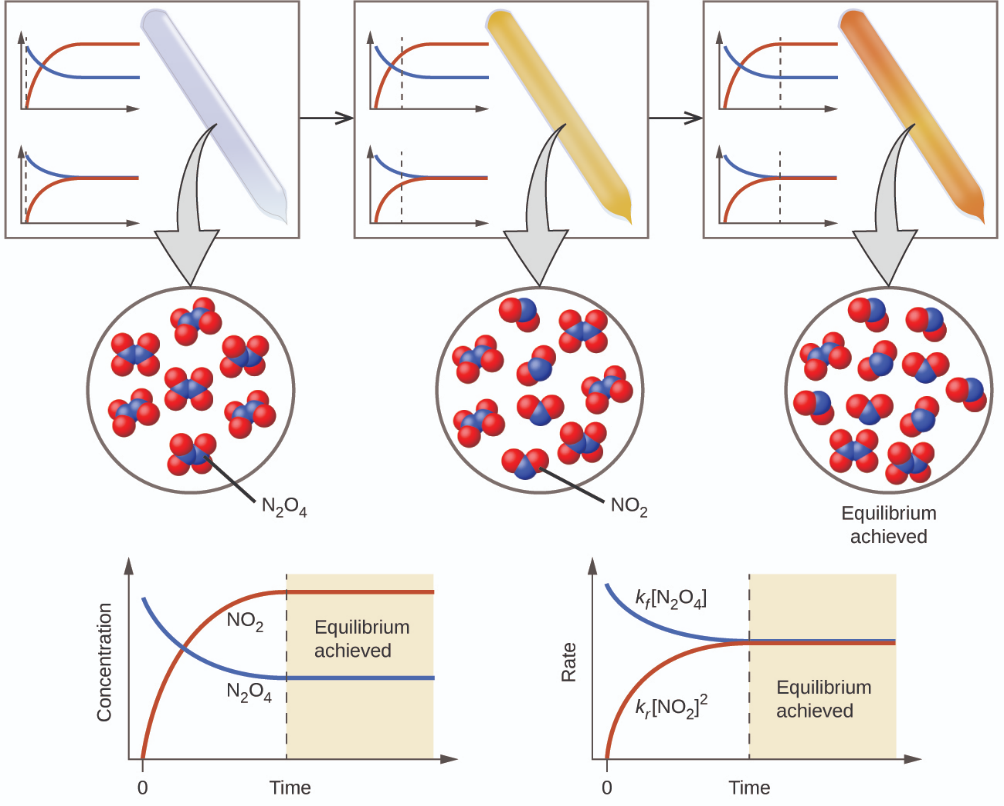
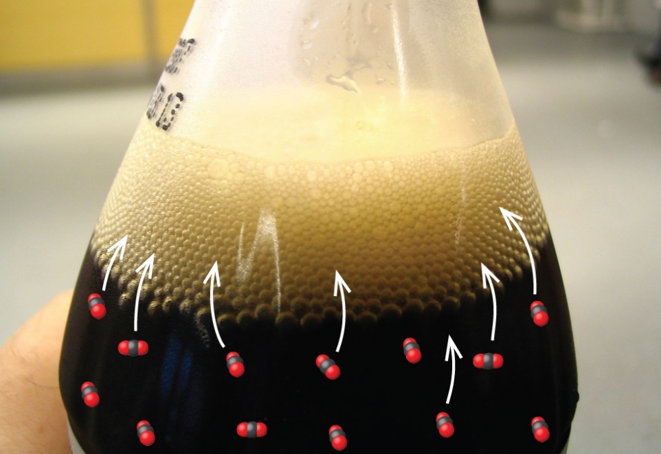
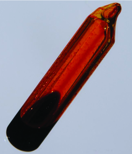
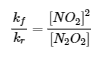
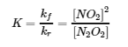
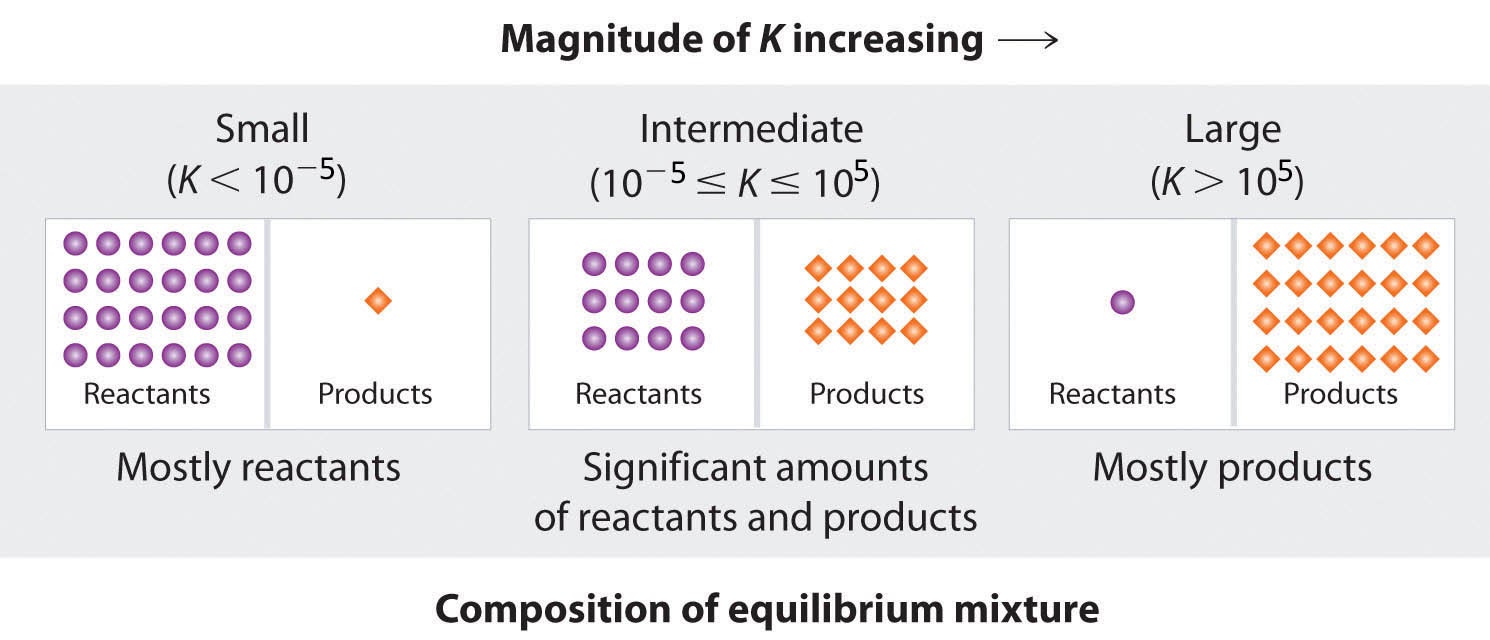
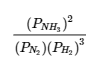


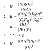
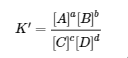
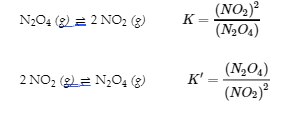
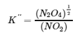
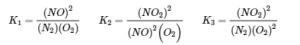
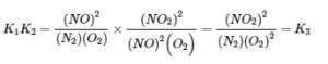
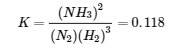
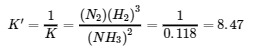
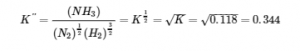
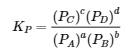
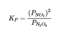
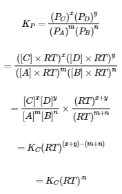

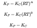

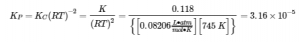
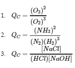
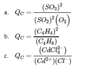
 = 0.10 mol/L, and [N2O4] = 0 mol/L. Thus,
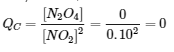
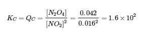
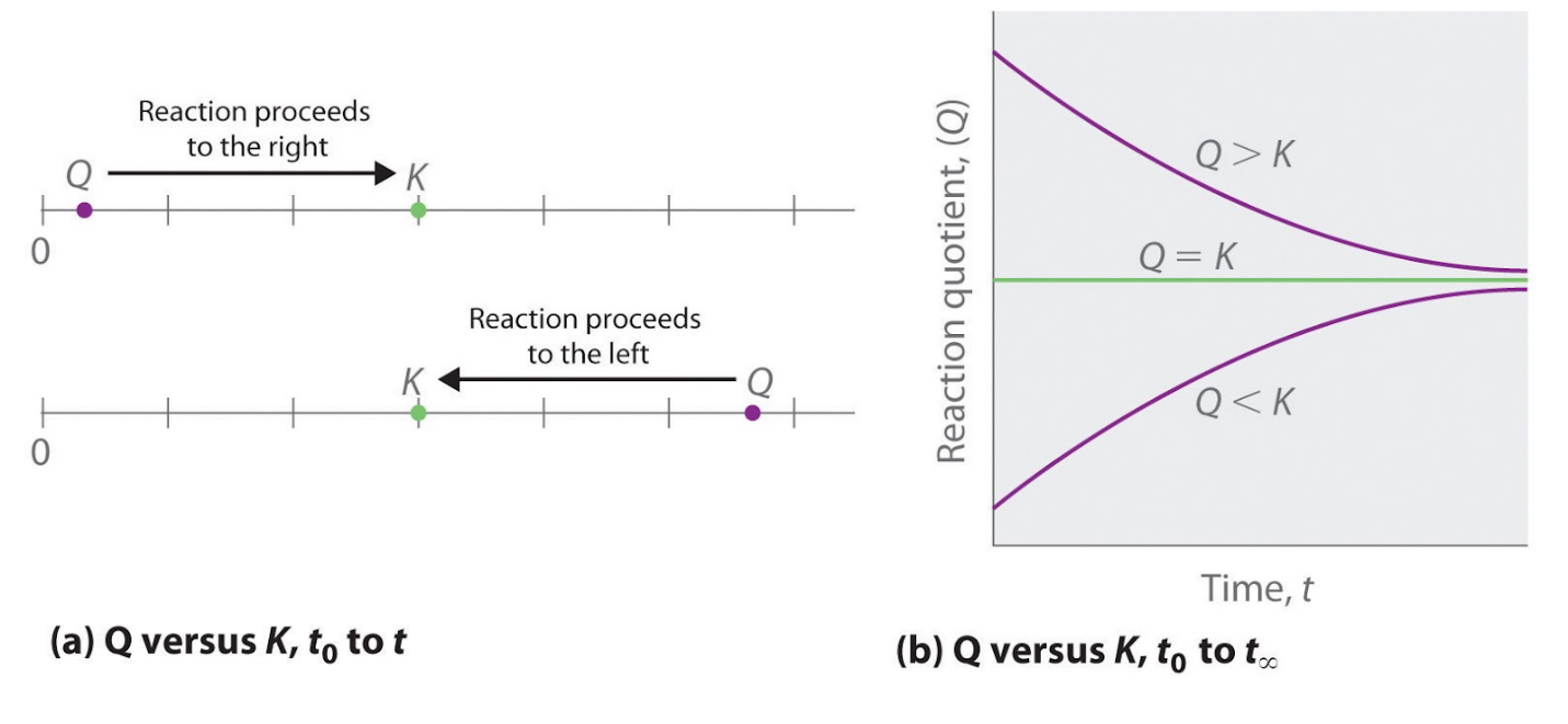
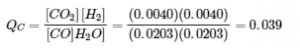

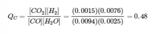
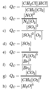
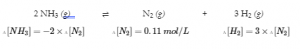
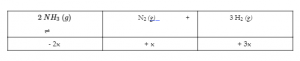
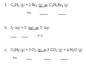
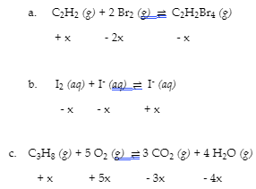
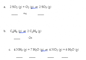
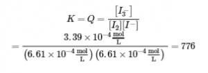
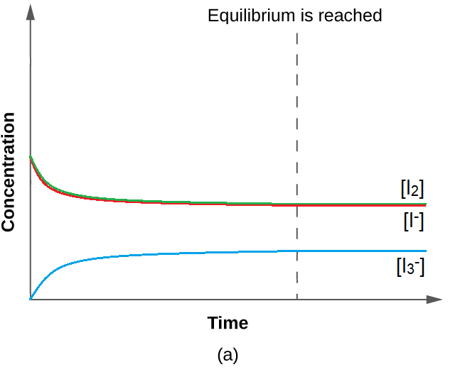
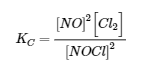
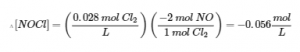
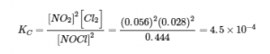
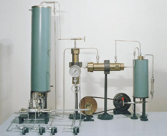
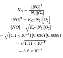
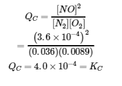
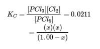
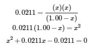
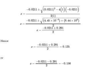
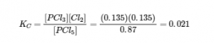
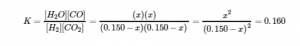
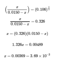
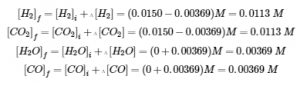
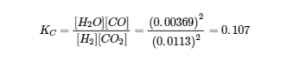
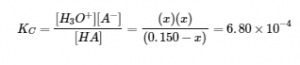
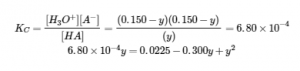
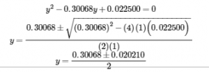
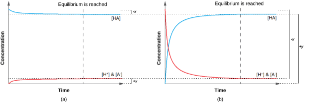

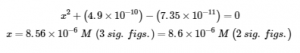
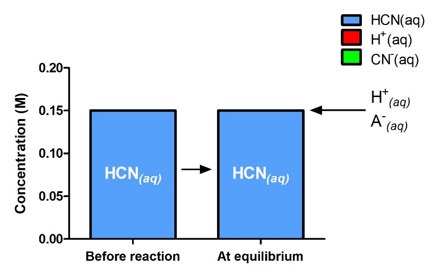
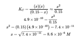
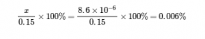
 W
W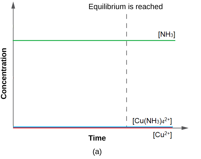
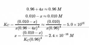
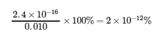
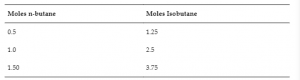
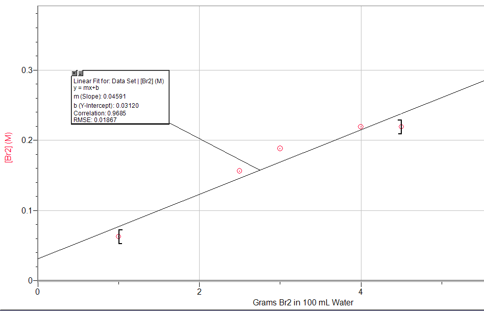
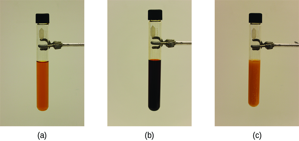
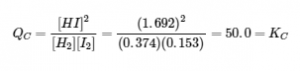
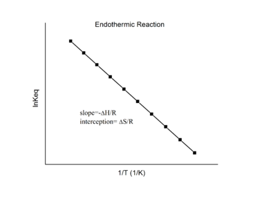
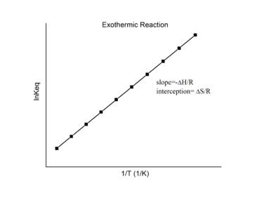
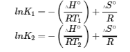
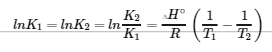
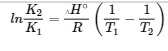

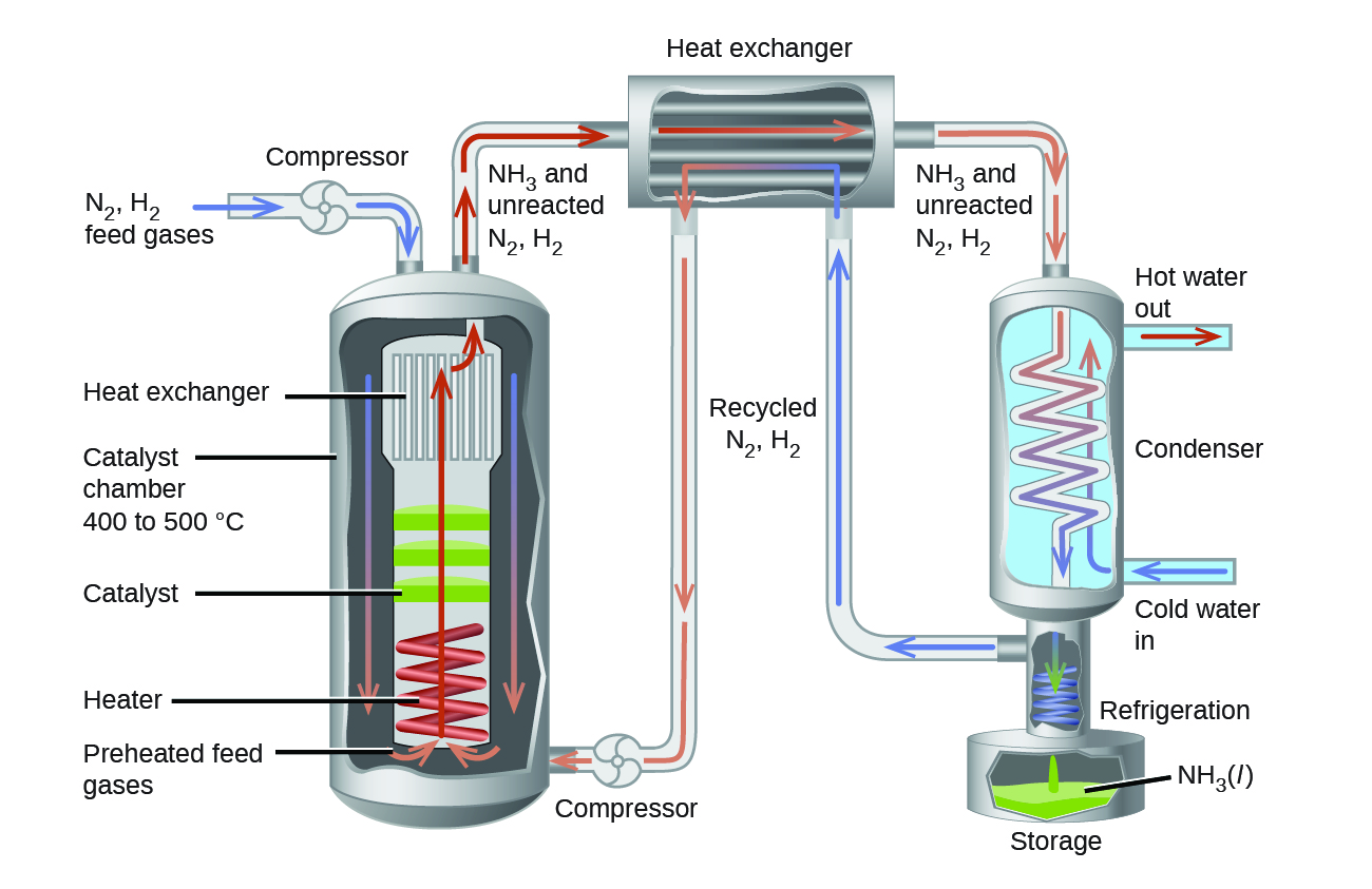
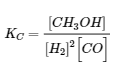
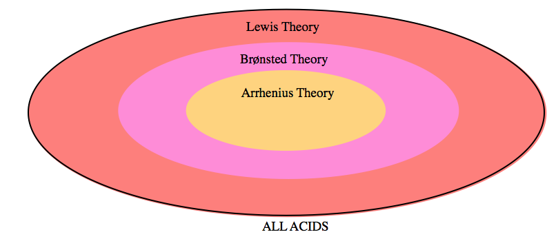
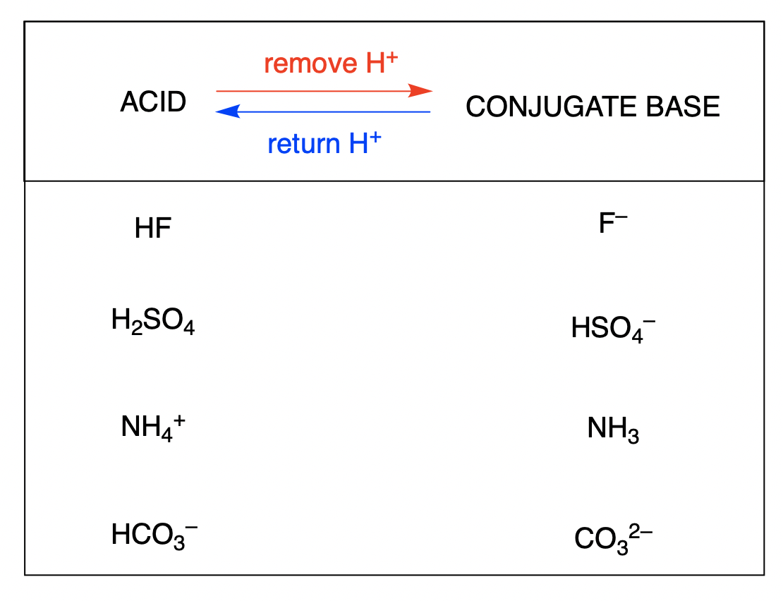
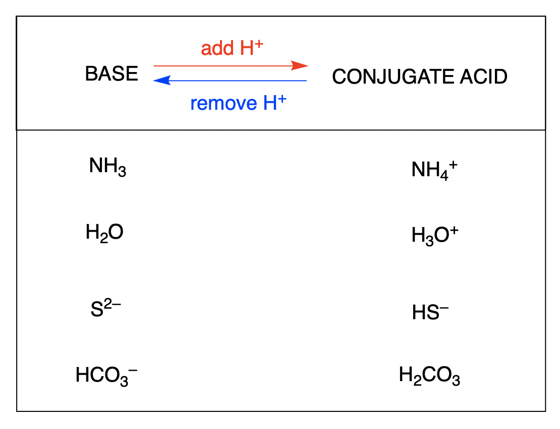
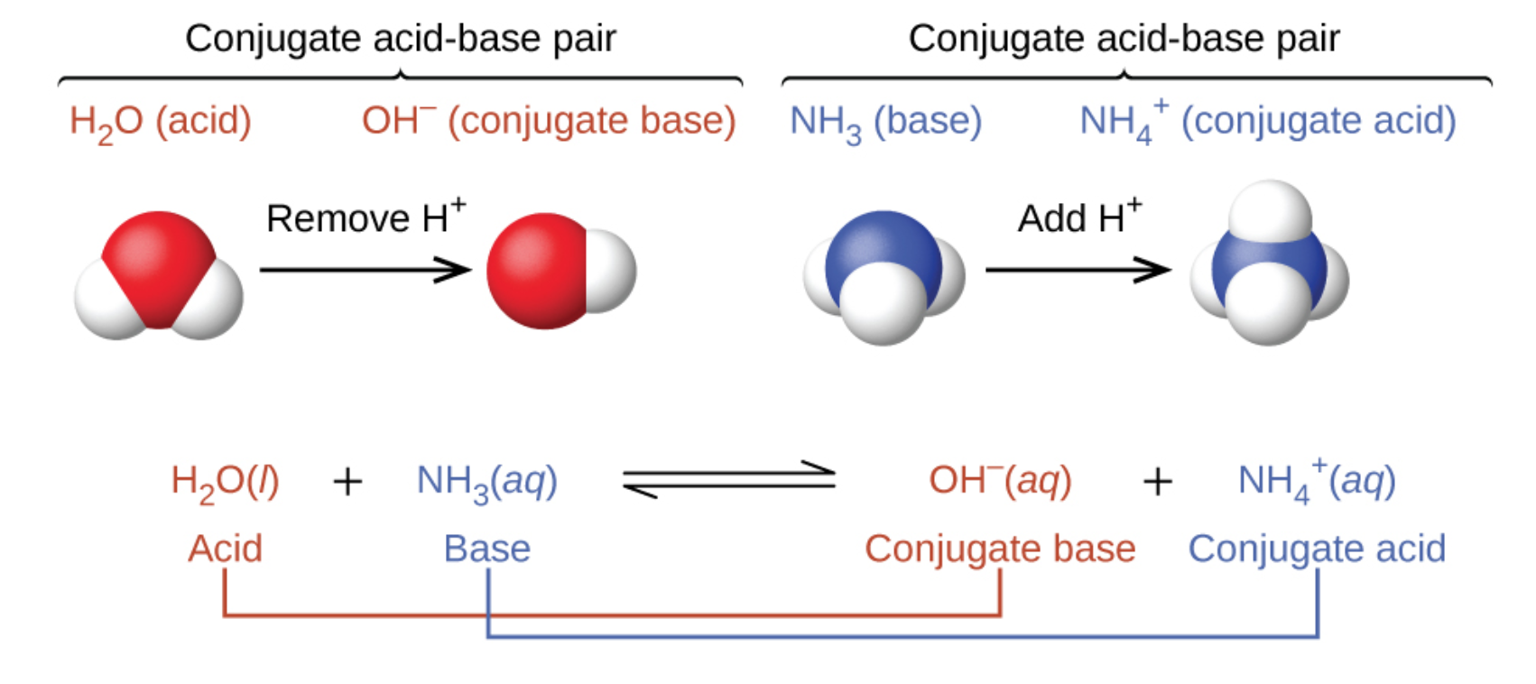
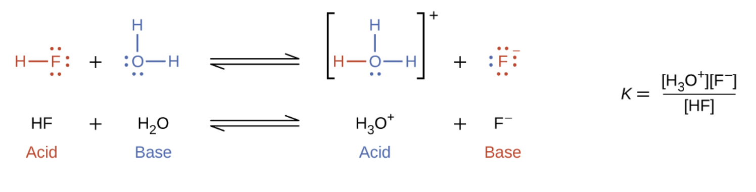
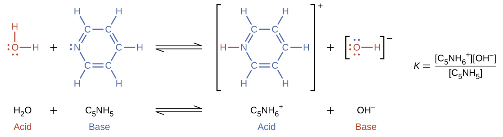
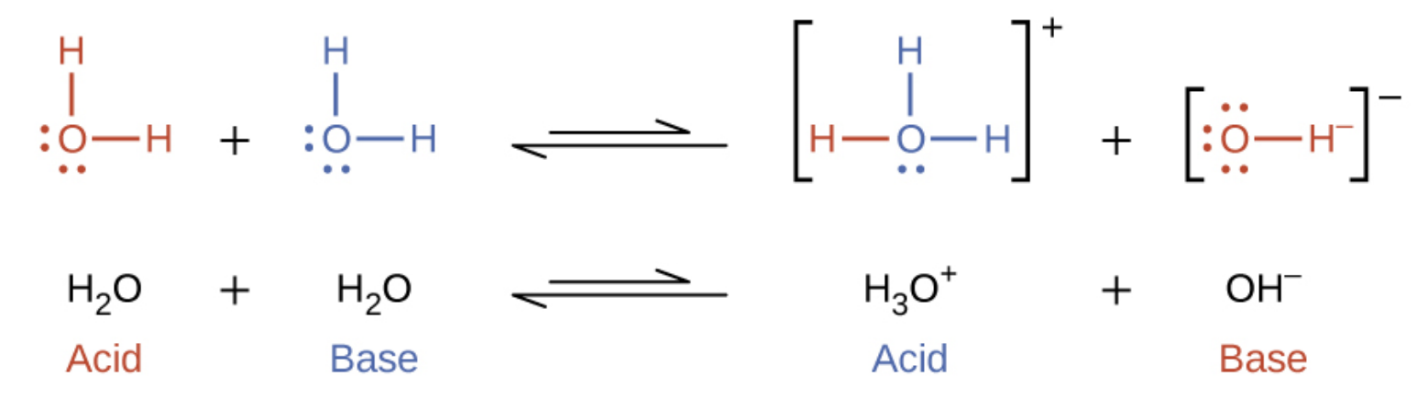
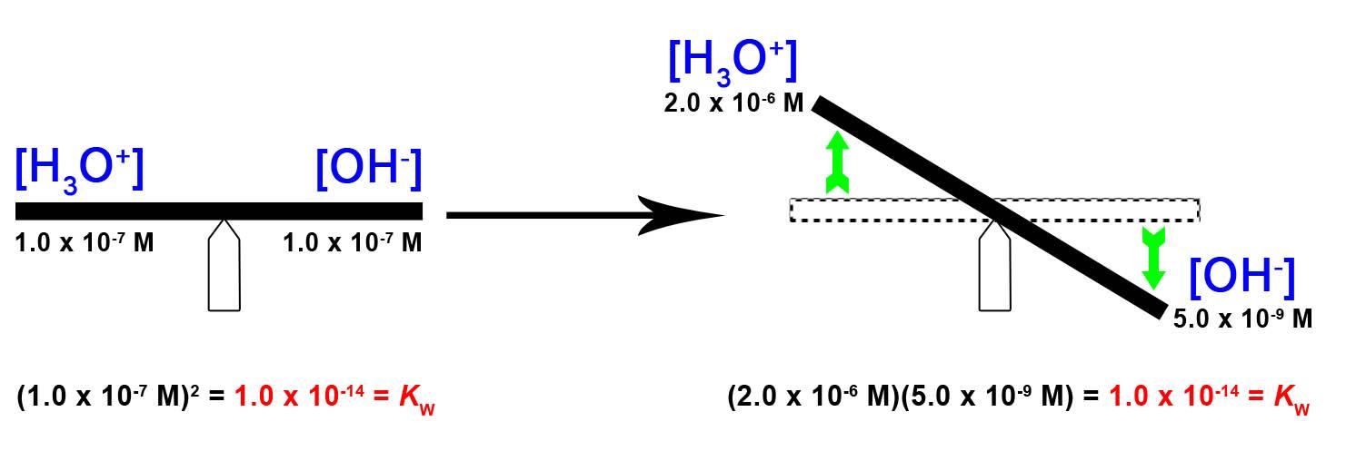
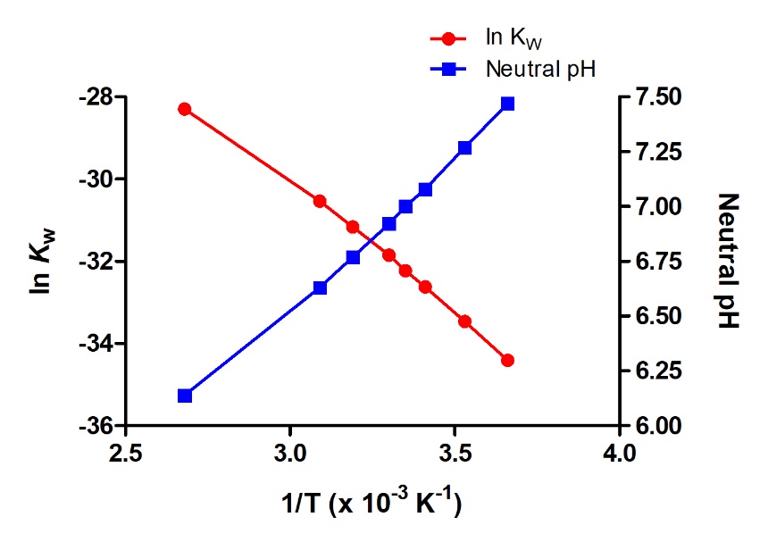
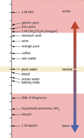
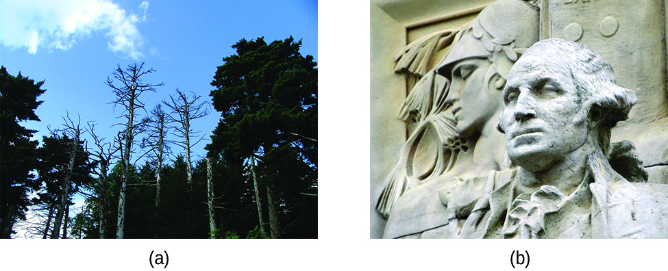
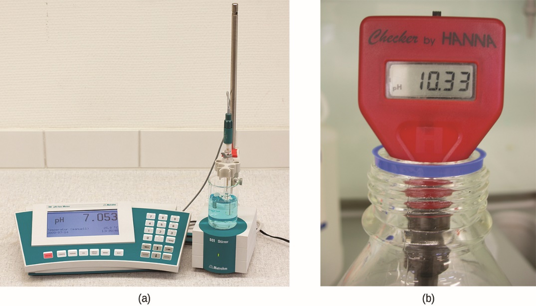
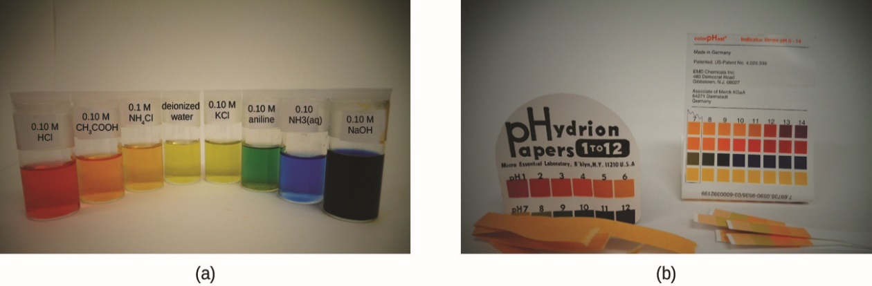
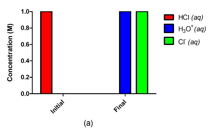
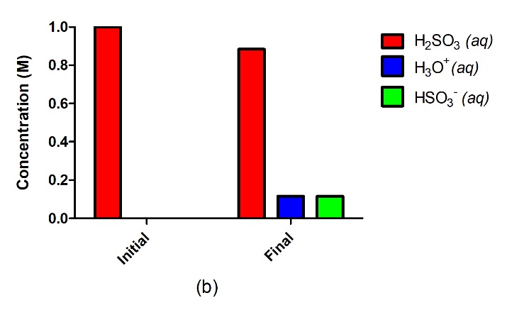
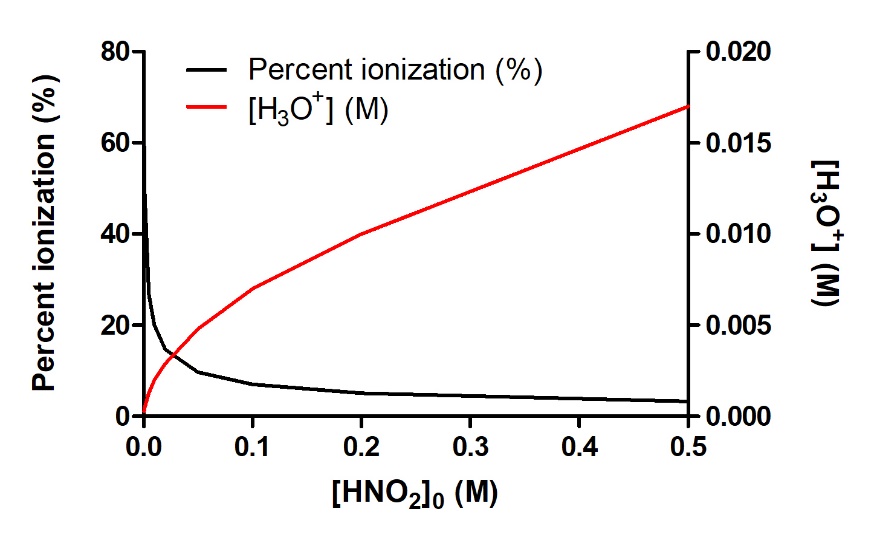
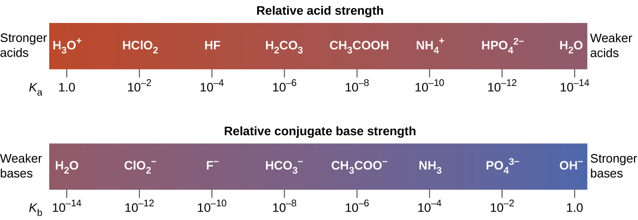
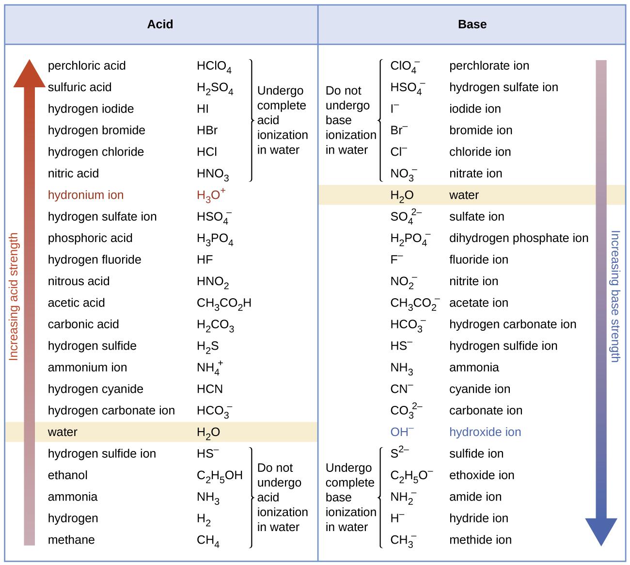
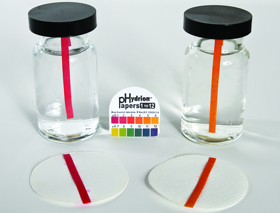
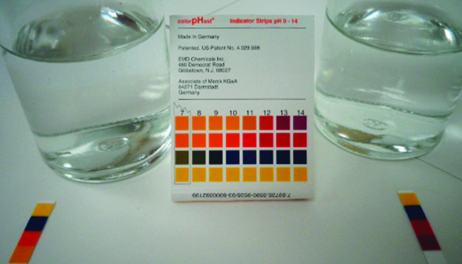
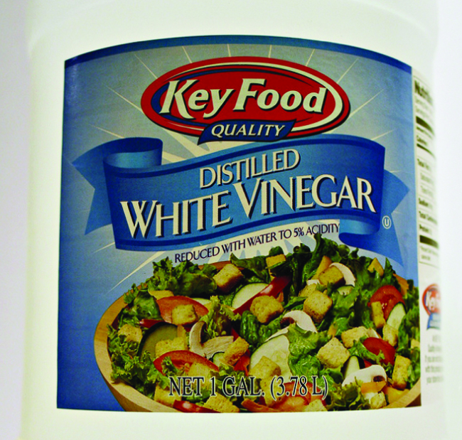
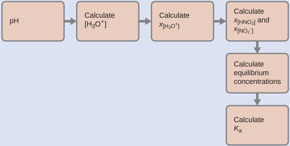

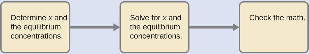
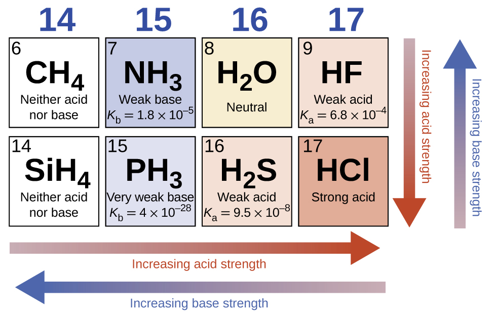
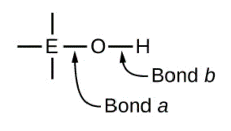
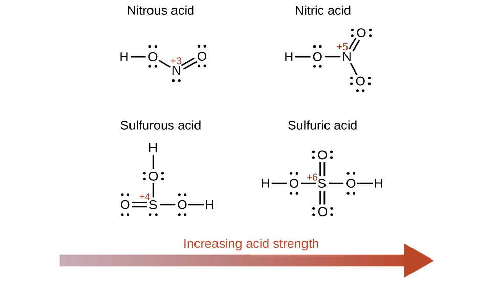
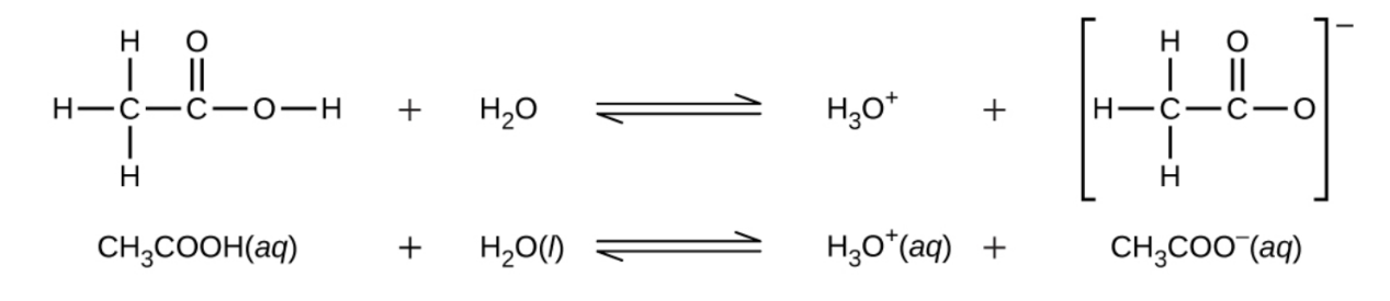
 NOTE: Ionizable (also known as acidic) protons are typically written at the beginning of a condensed chemical formula. Examples of this include H2SO4, which is diprotic, and H3PO4, which is triprotic. Occasionally, some chemical formulae do not follow this pattern. This is usually due to historical reasons where the chemical formula has been written a certain way for several years. For example, acetic acid can be written HC2H3O2, CH3CO2H, or CH3COOH. When in doubt, check the literature for the correct formula.
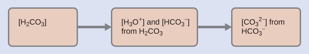

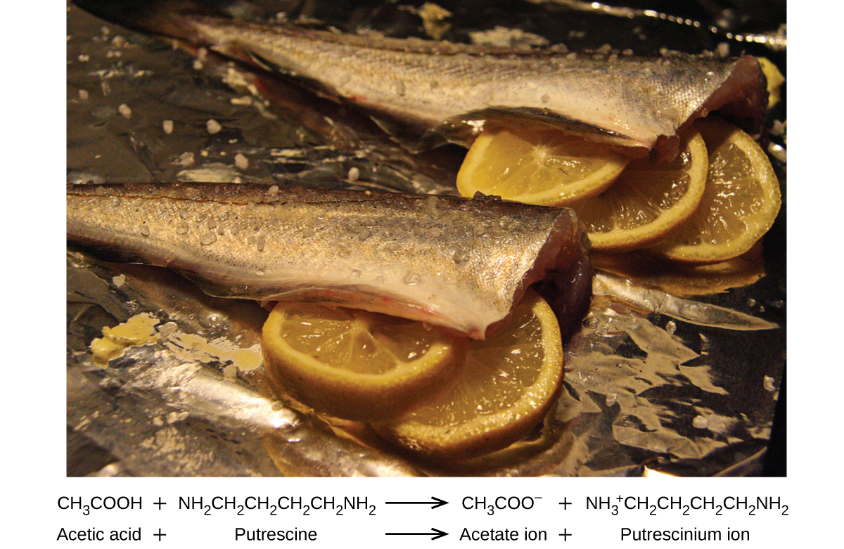
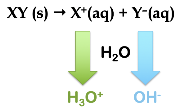

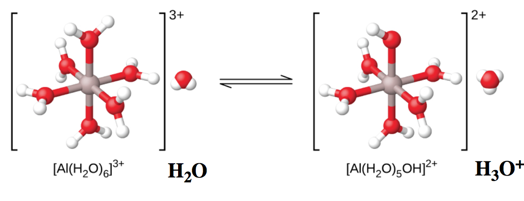
 P
P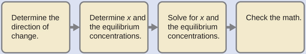
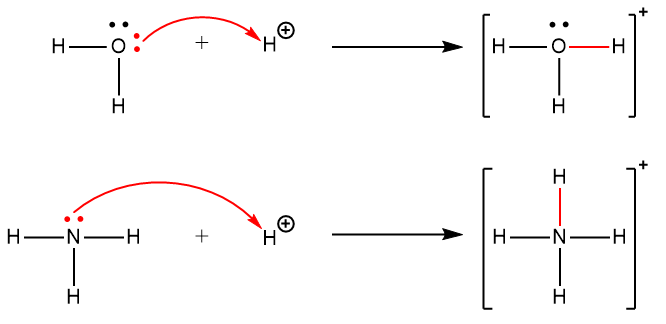
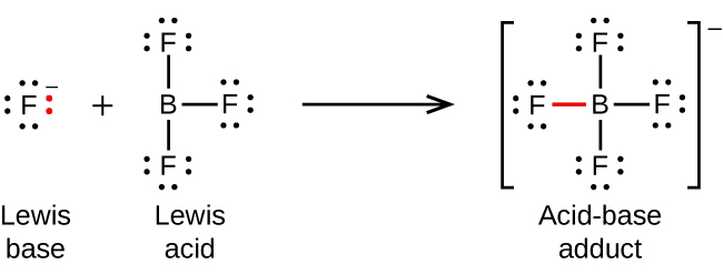
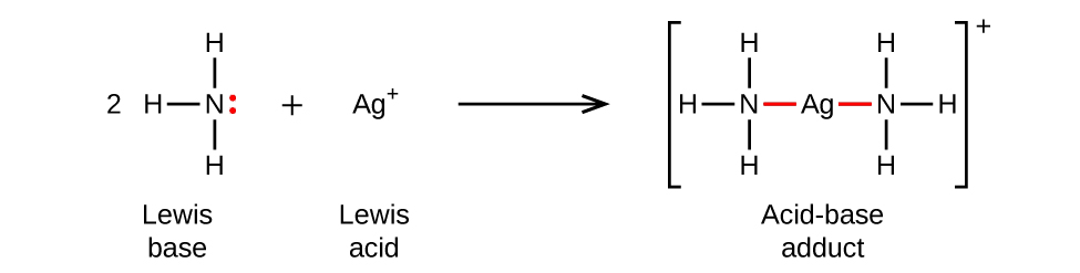
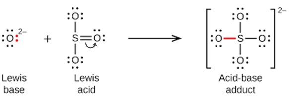
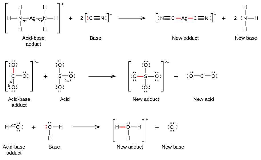
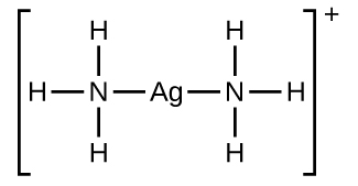
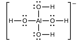
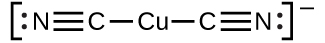
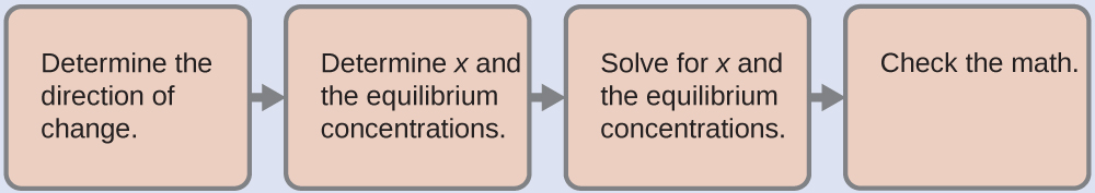
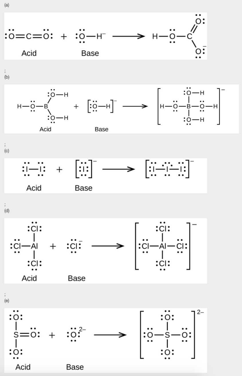
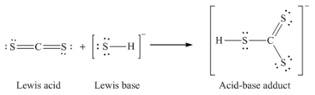
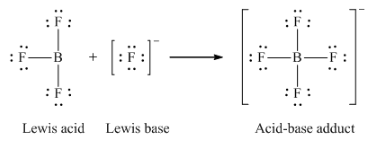
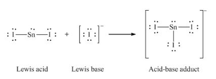
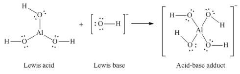
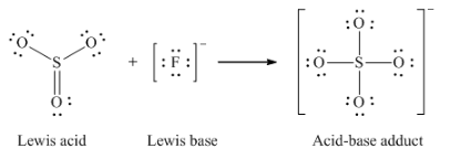
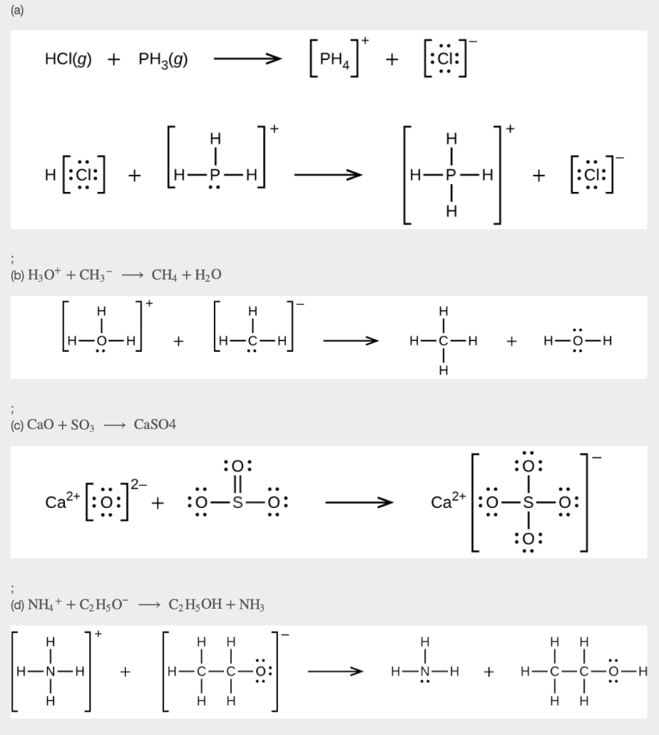
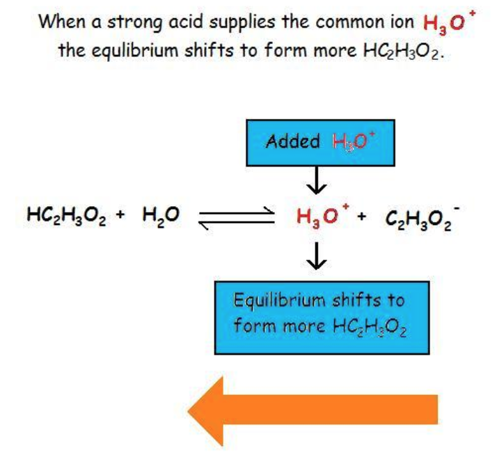
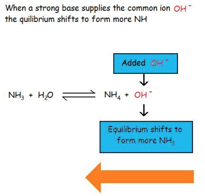
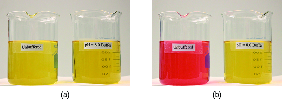

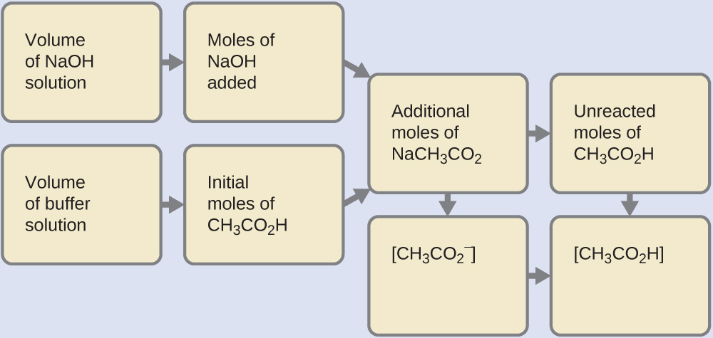
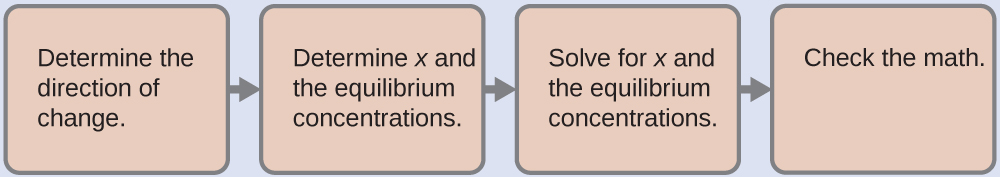
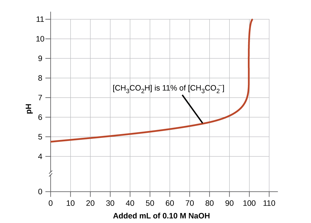
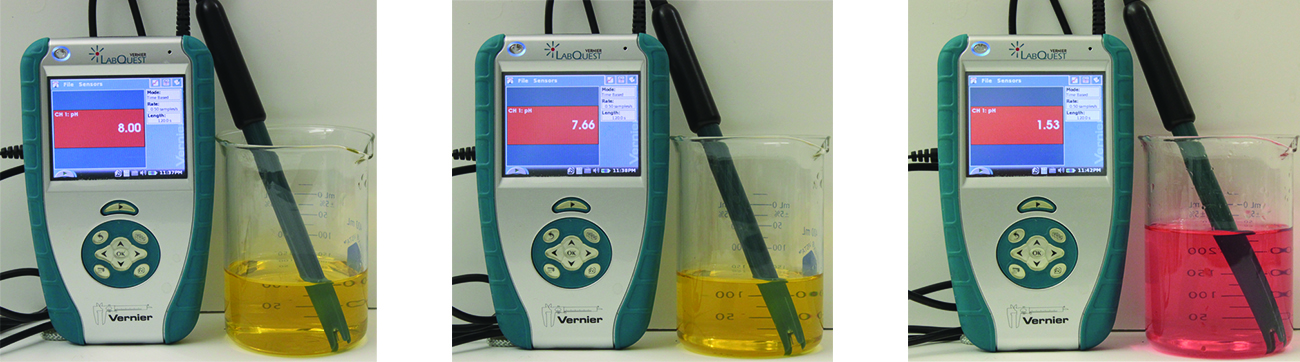
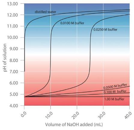
 CHM1311 Laboratory | Experiment #3: Equilibria
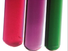
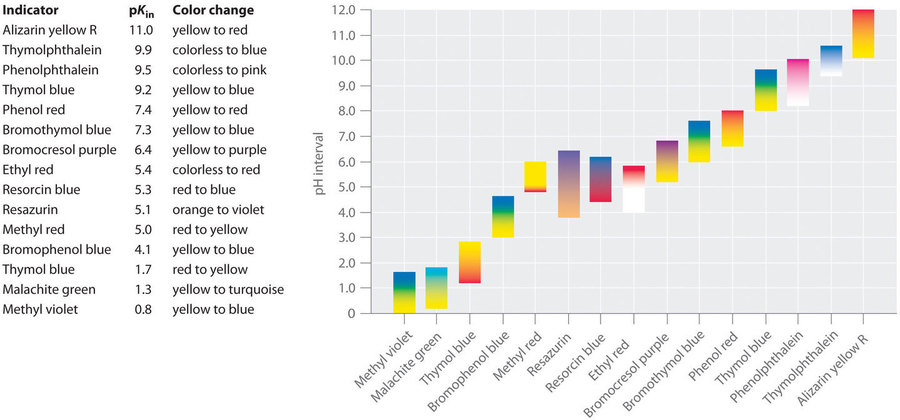
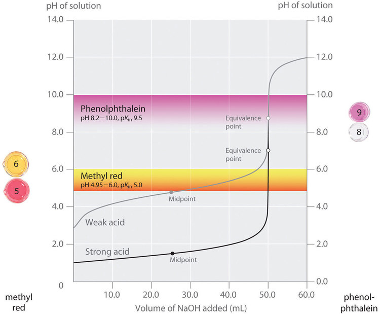
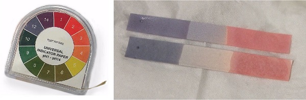
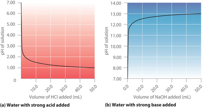
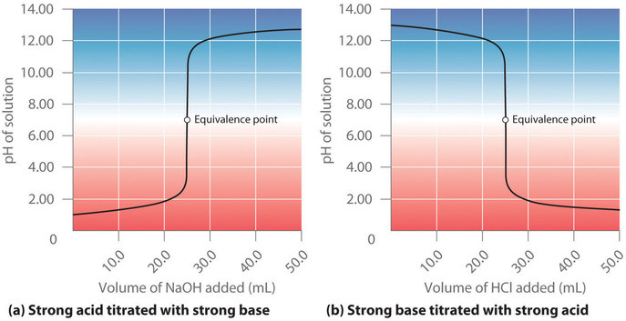
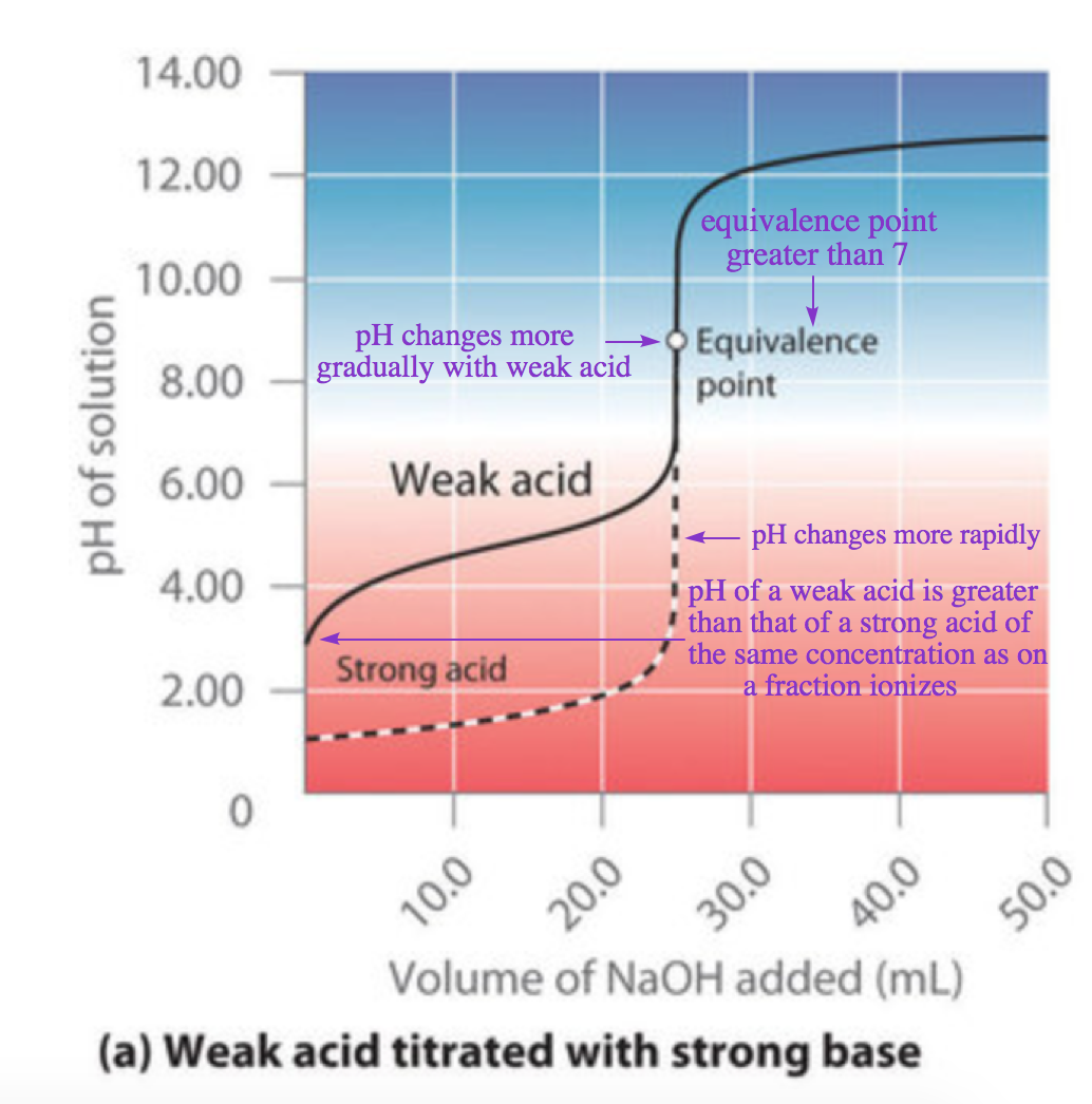
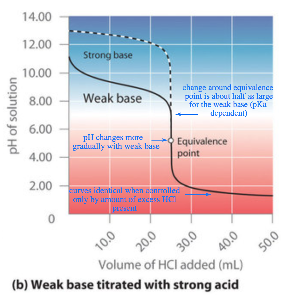
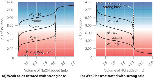
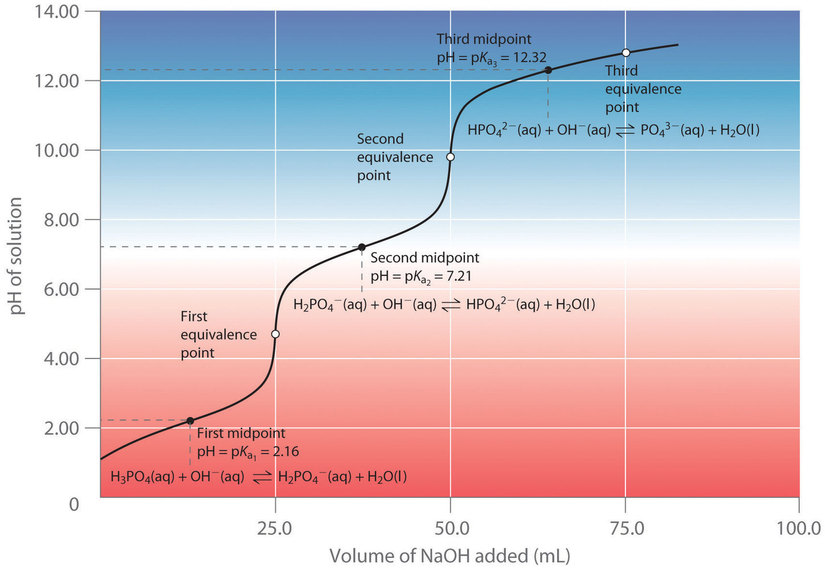
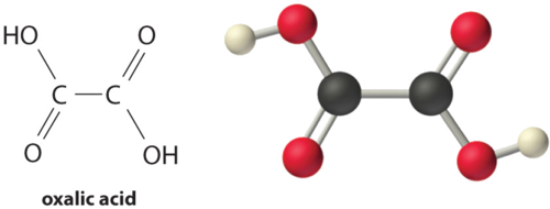
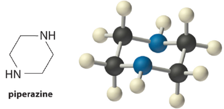
 CHM1311 Laboratory | Experiment #4: Acid Base Titrations
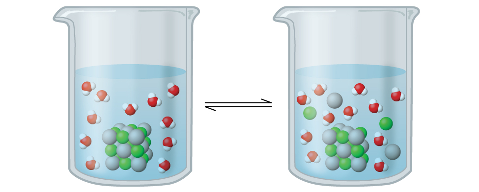
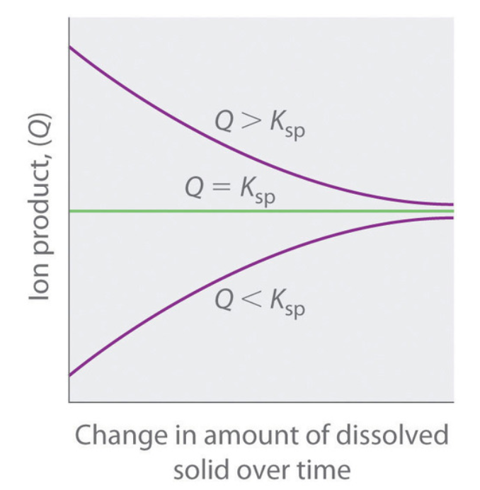
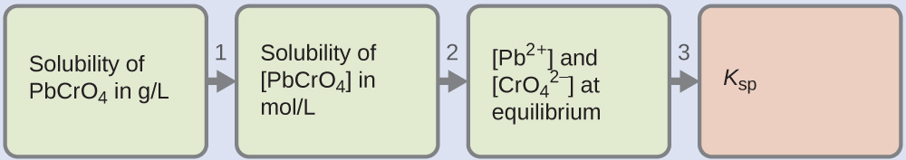

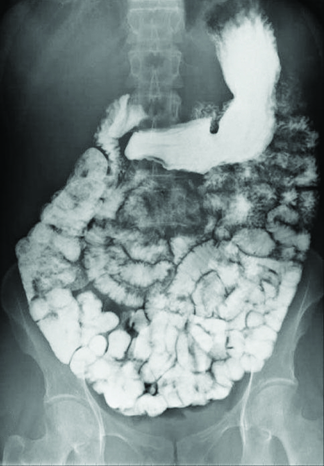
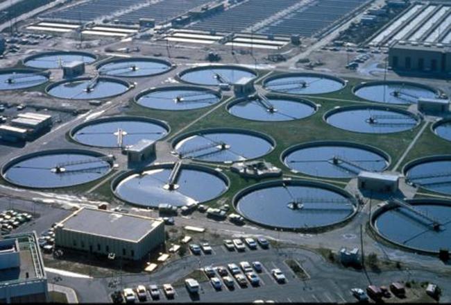
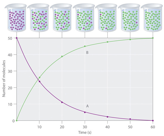
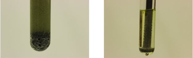
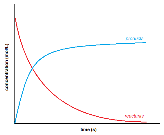
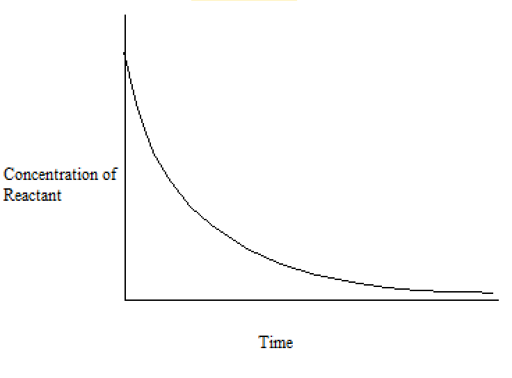
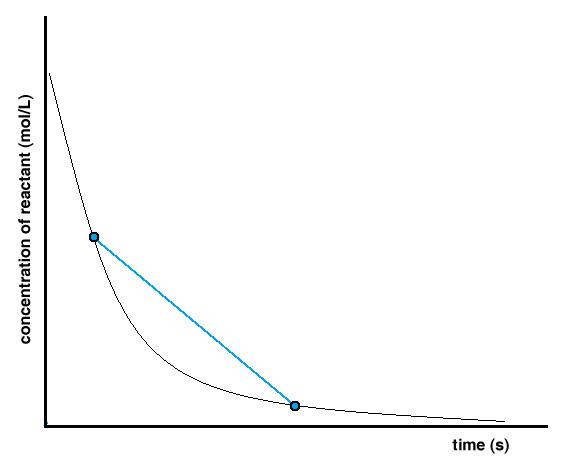
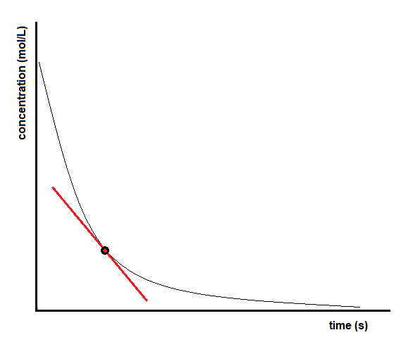
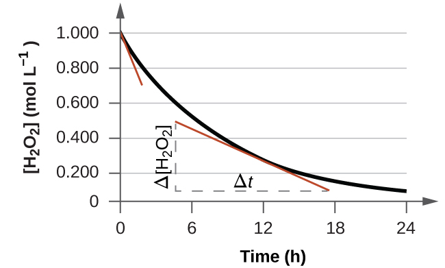
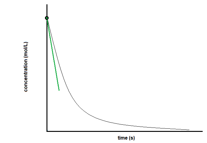
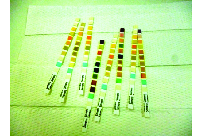
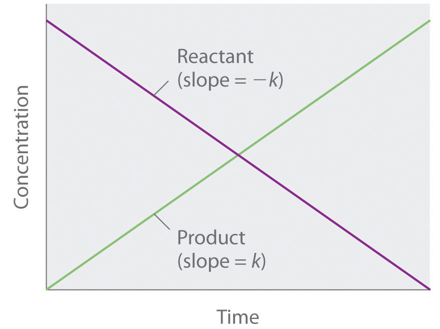
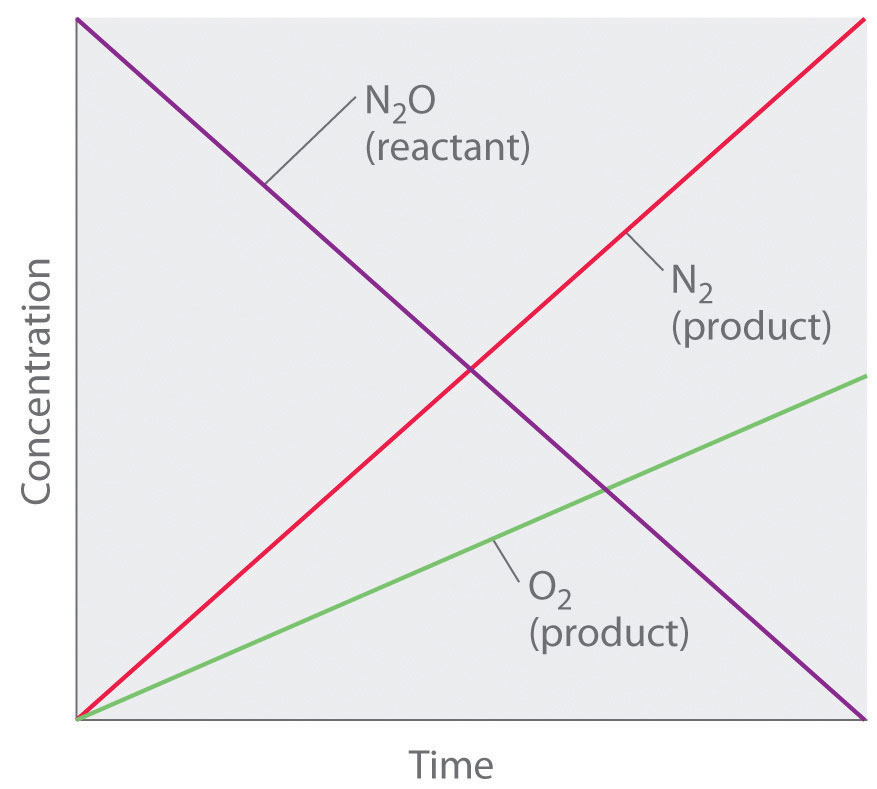
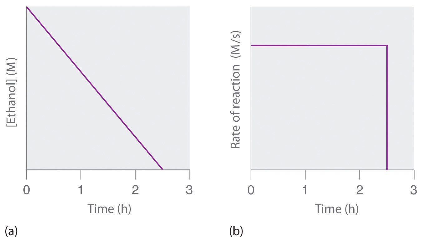
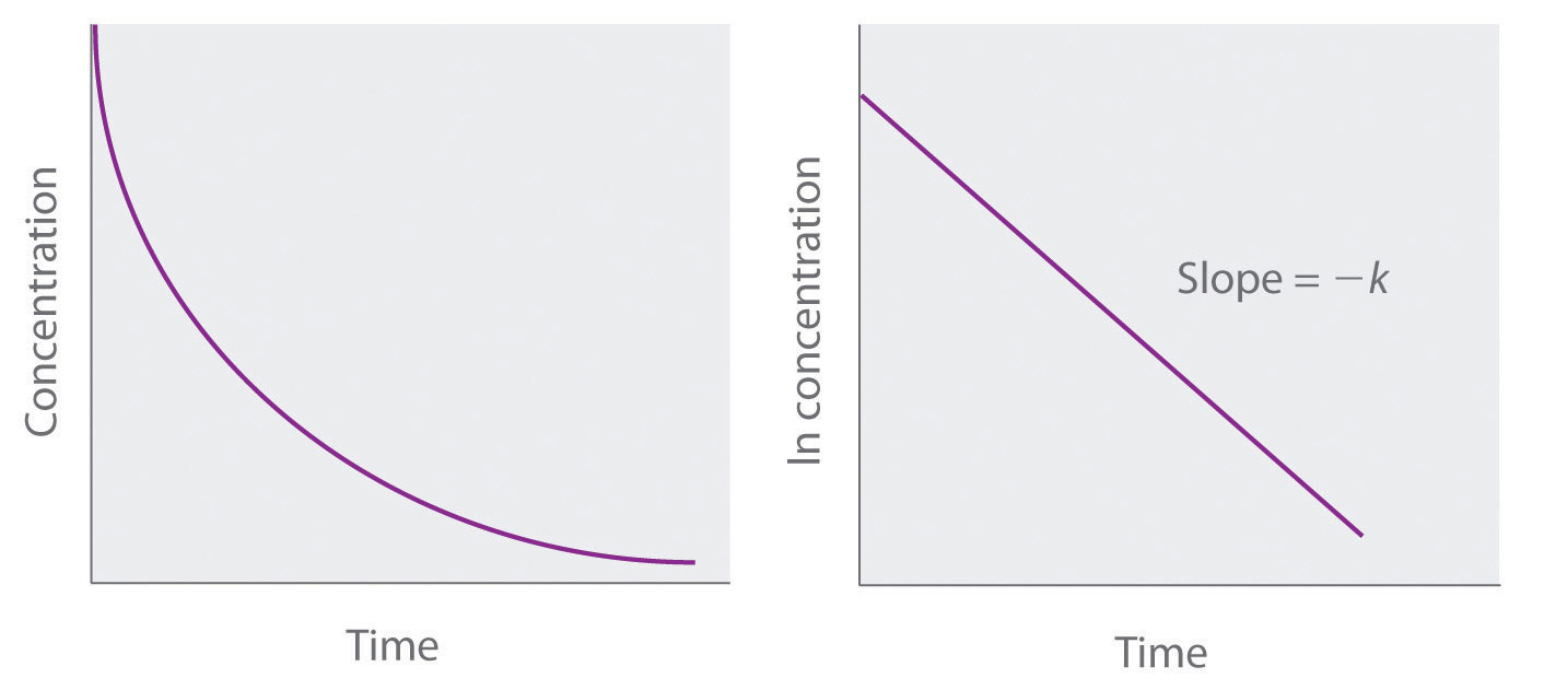
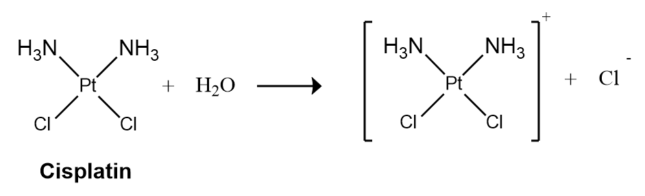
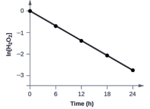
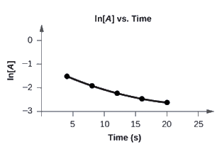
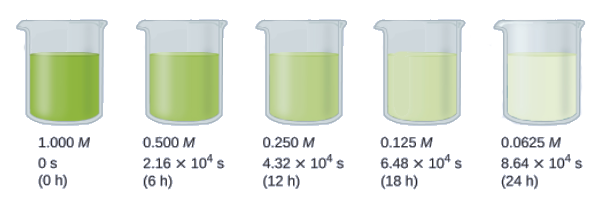
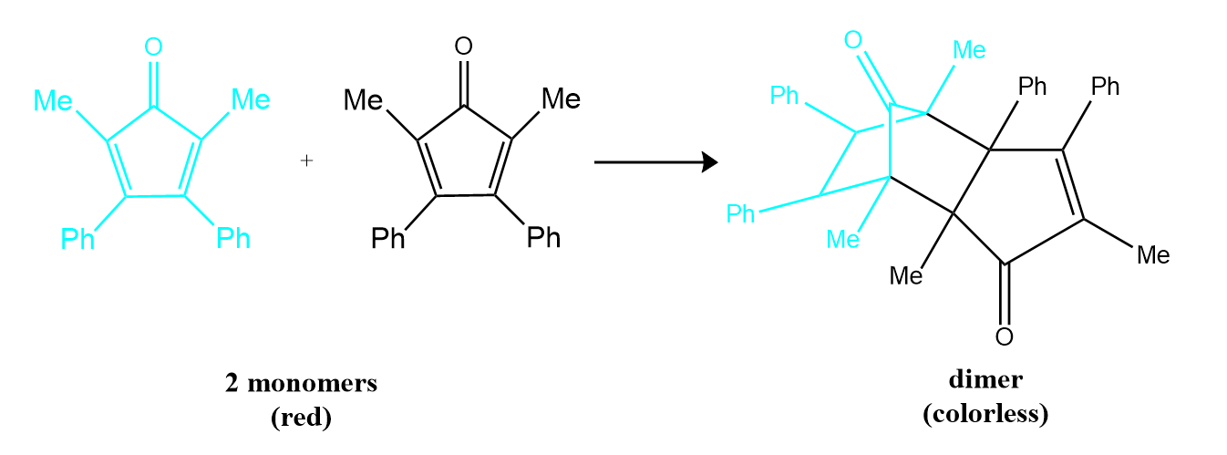
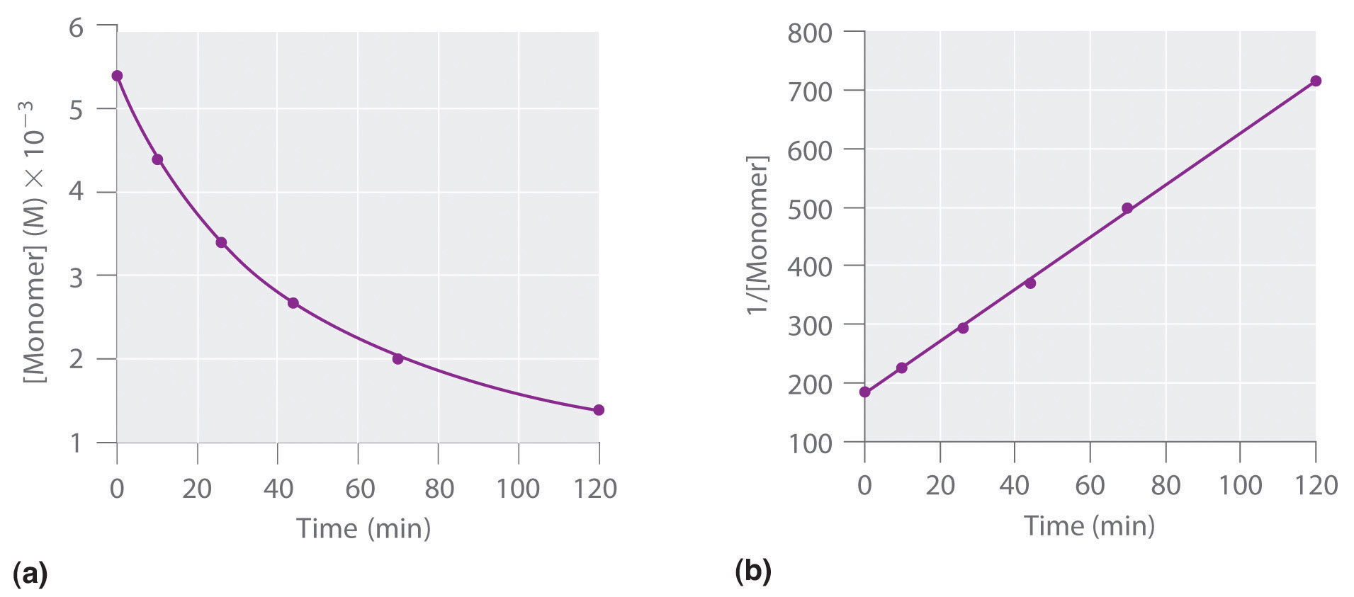
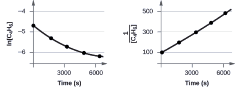
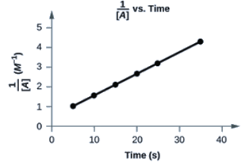
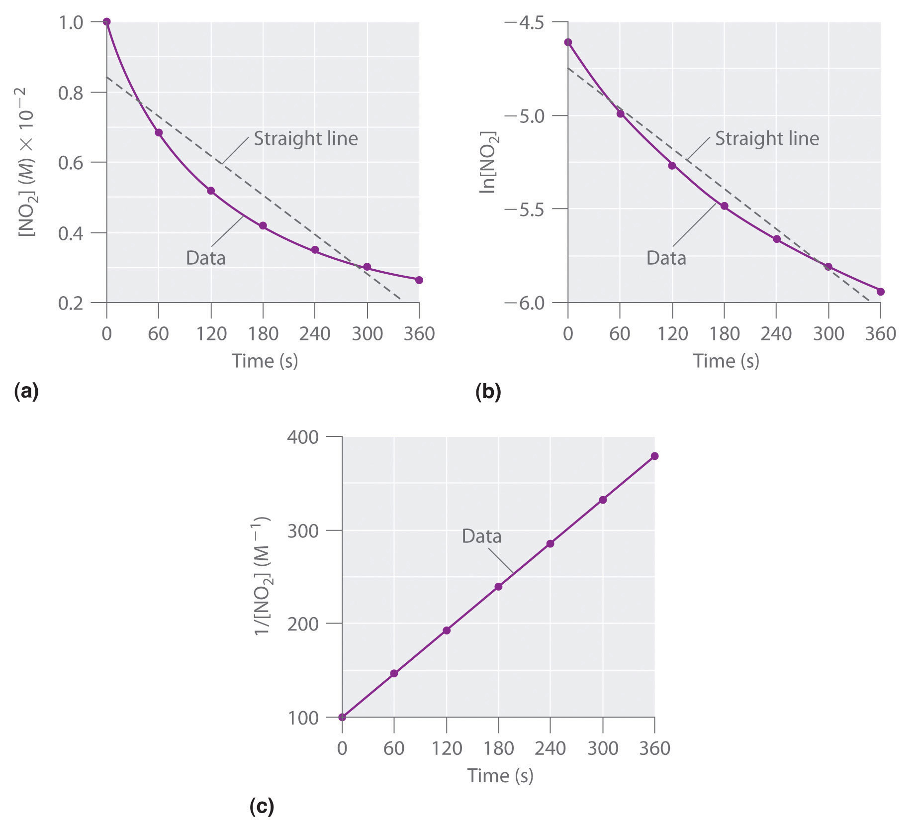
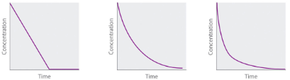
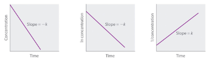
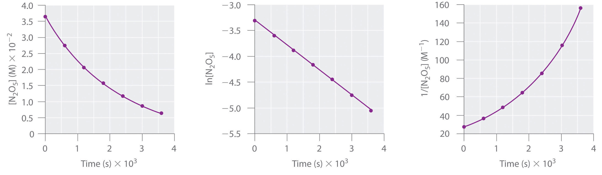
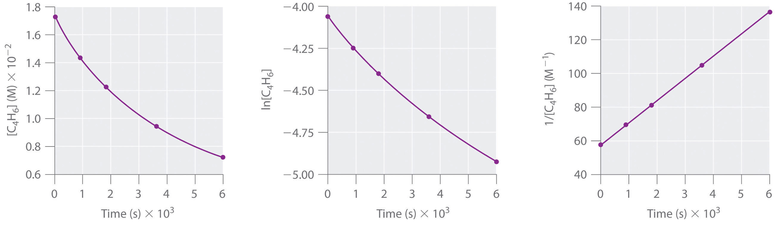
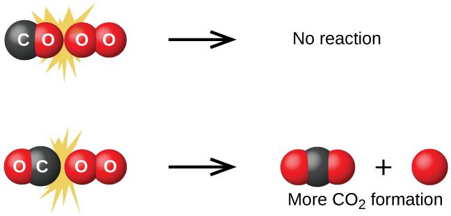
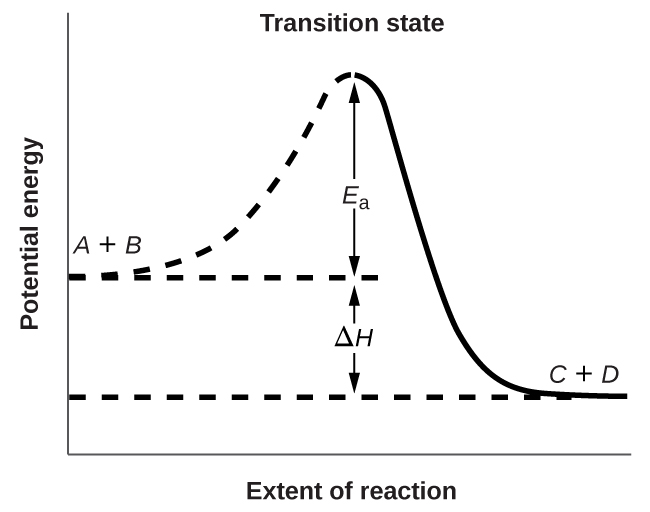
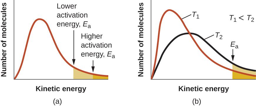
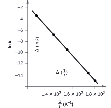
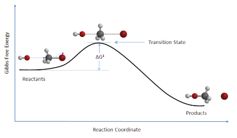
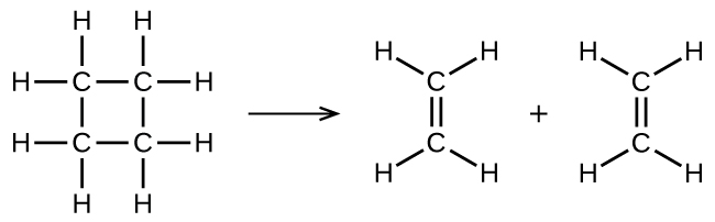
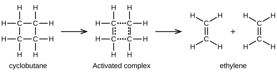
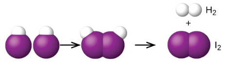
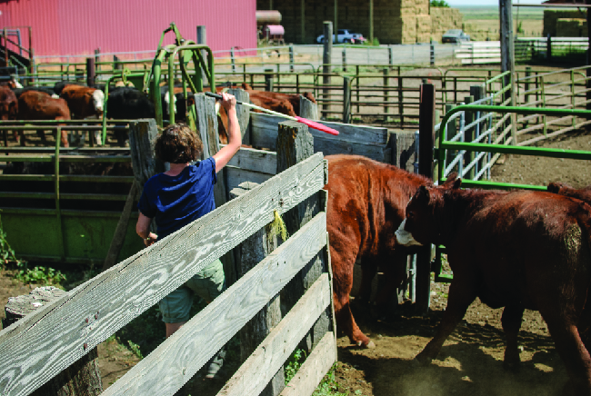
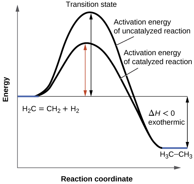
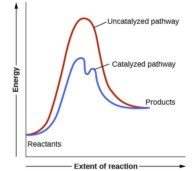
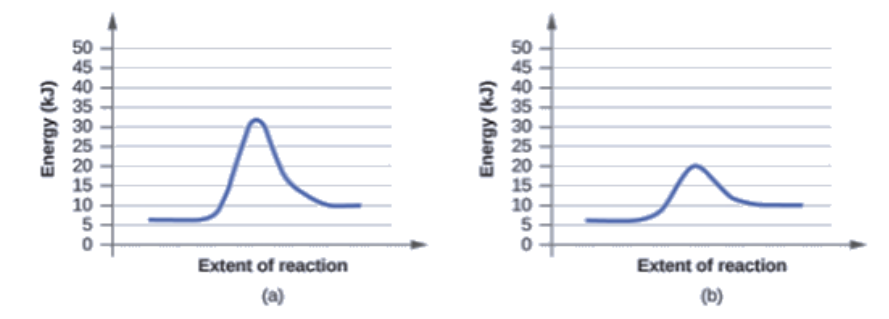
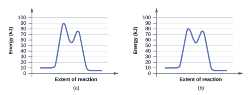
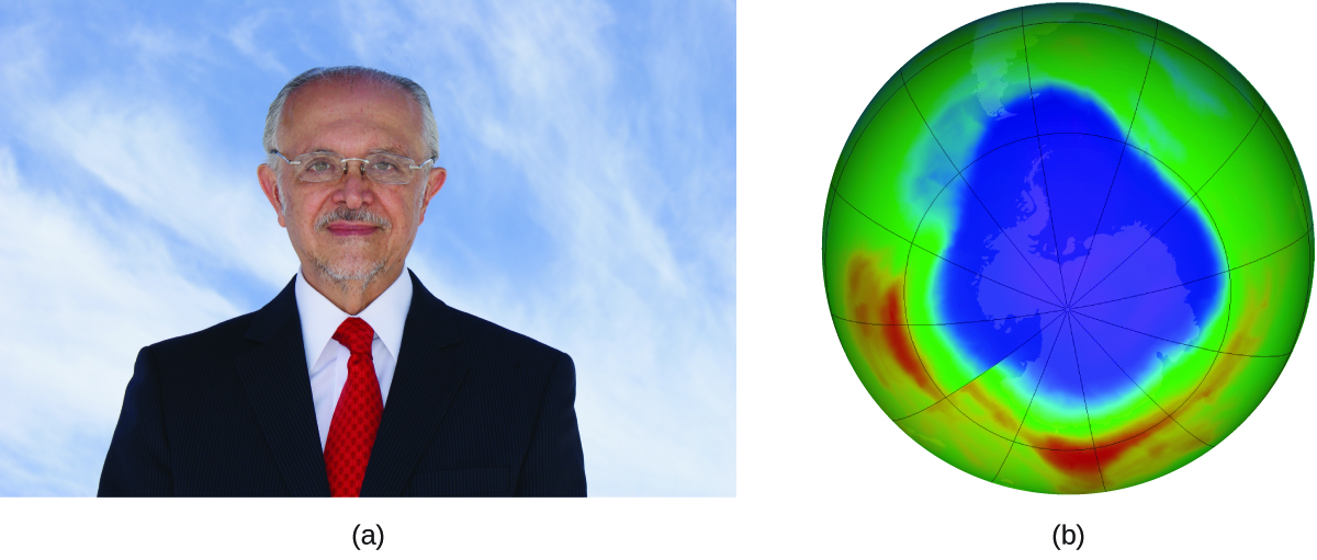
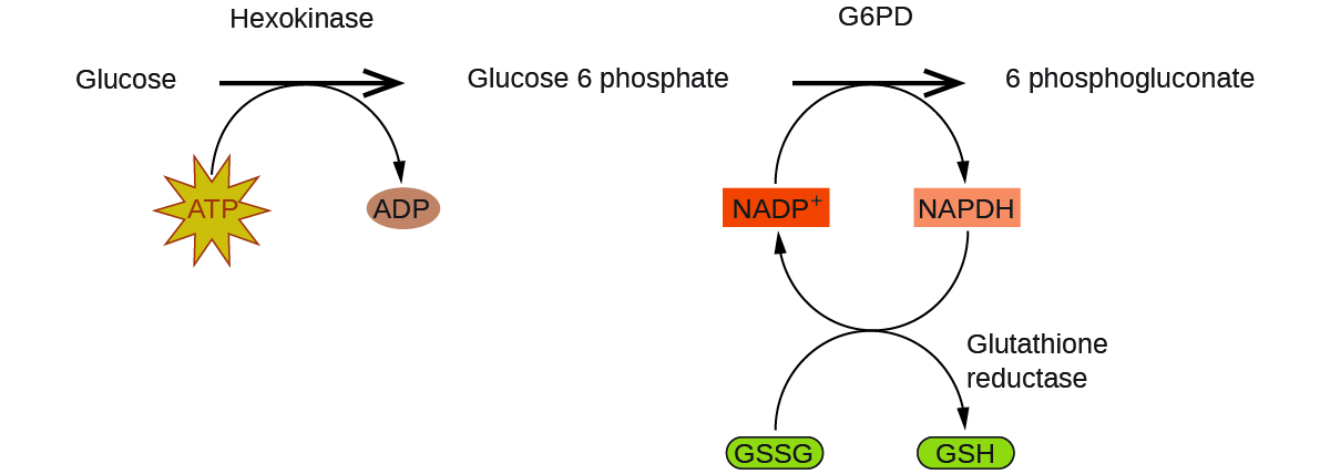
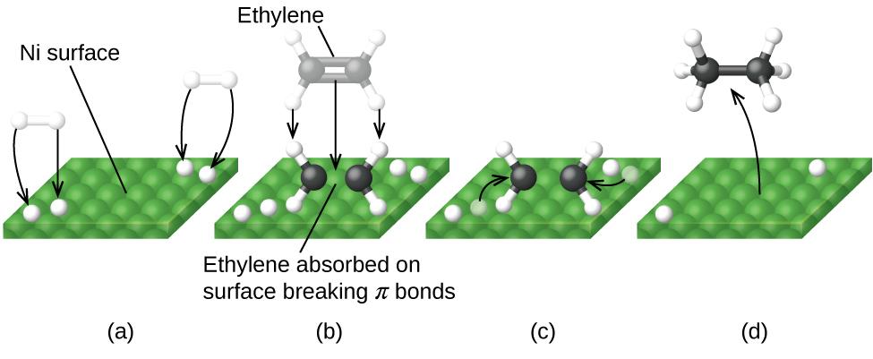
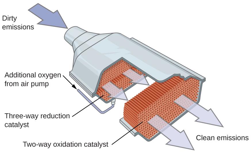
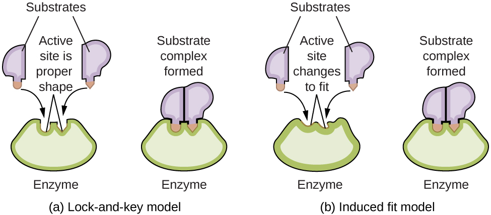

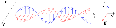
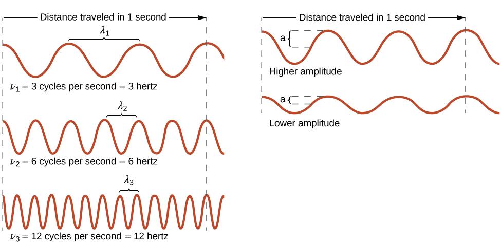
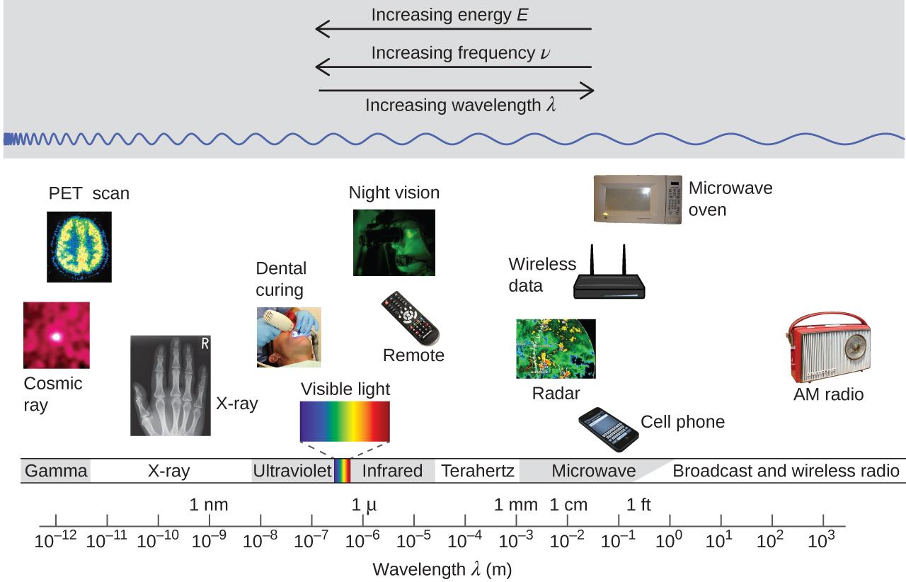
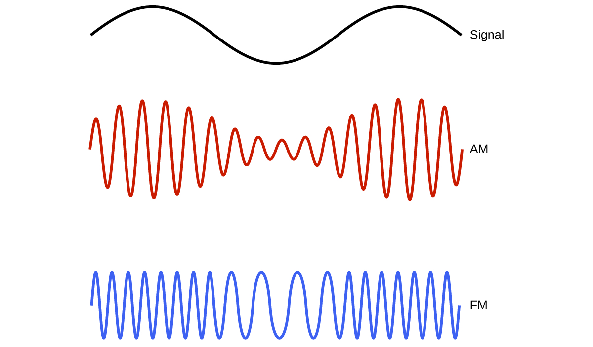

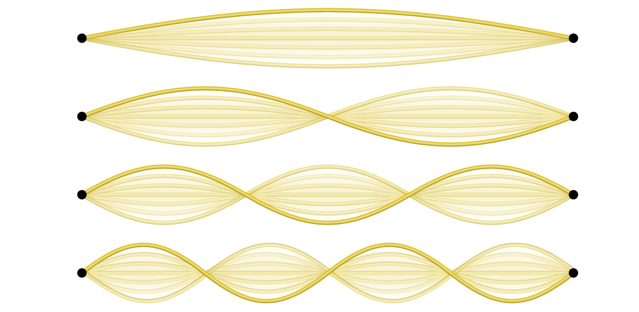
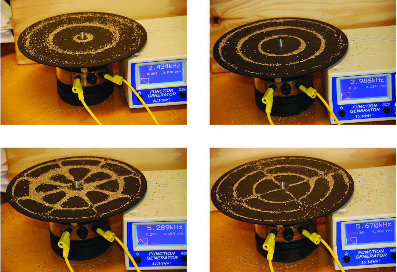
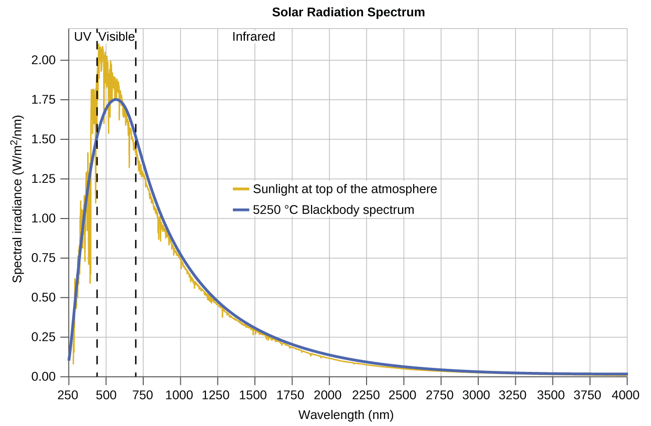
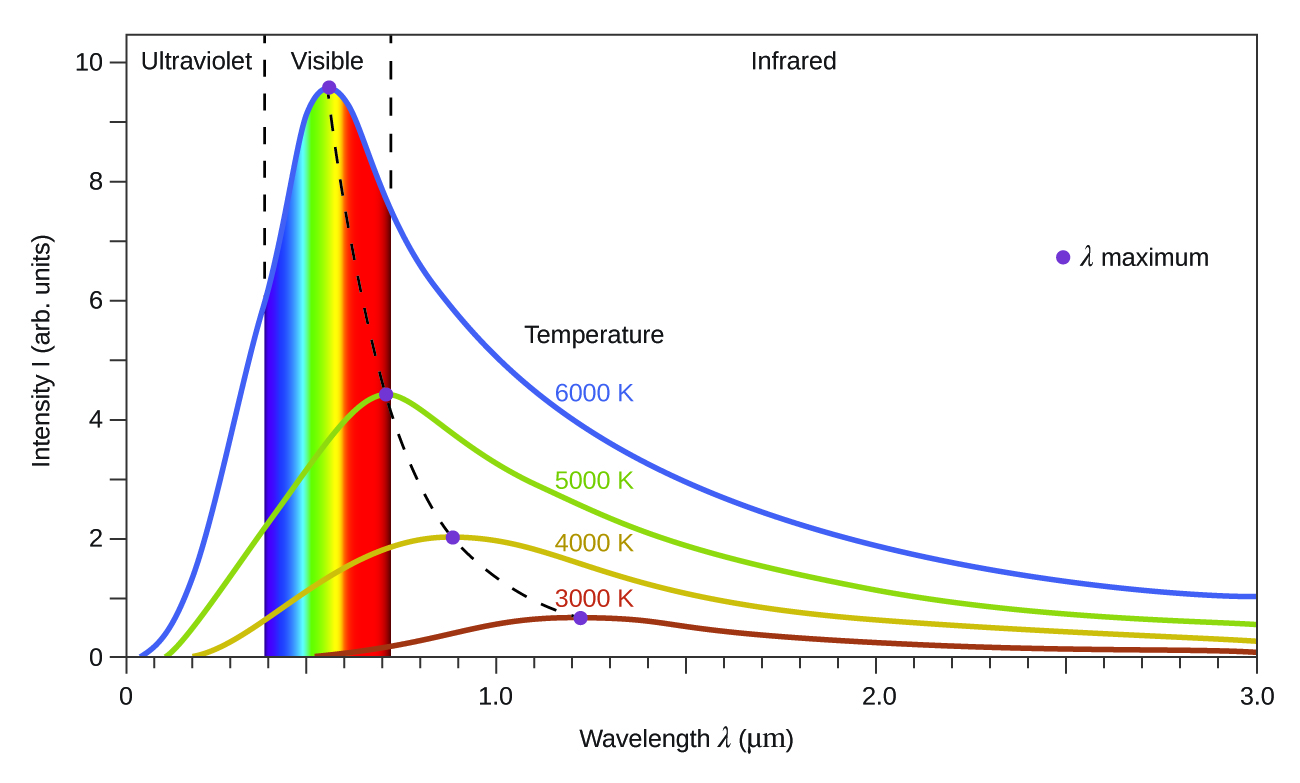
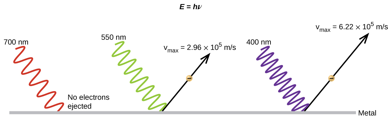

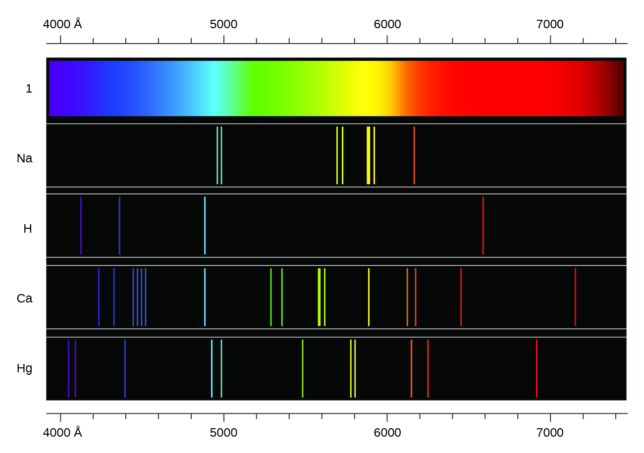
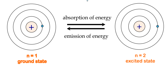
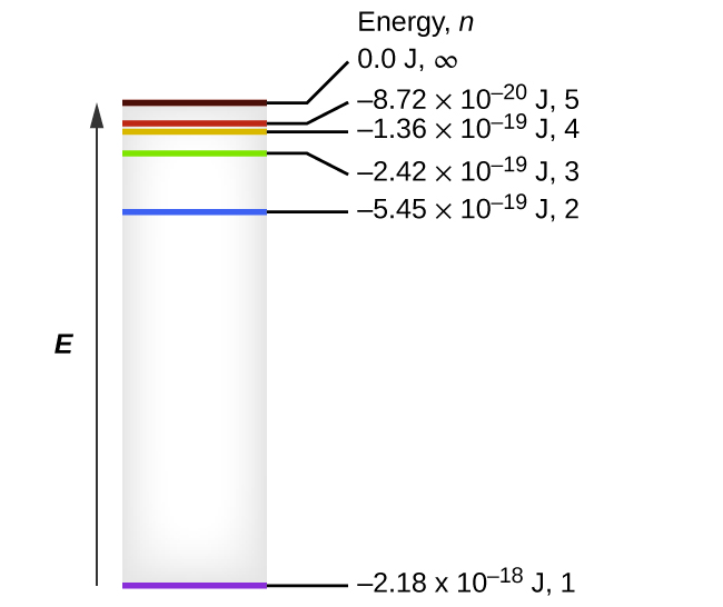
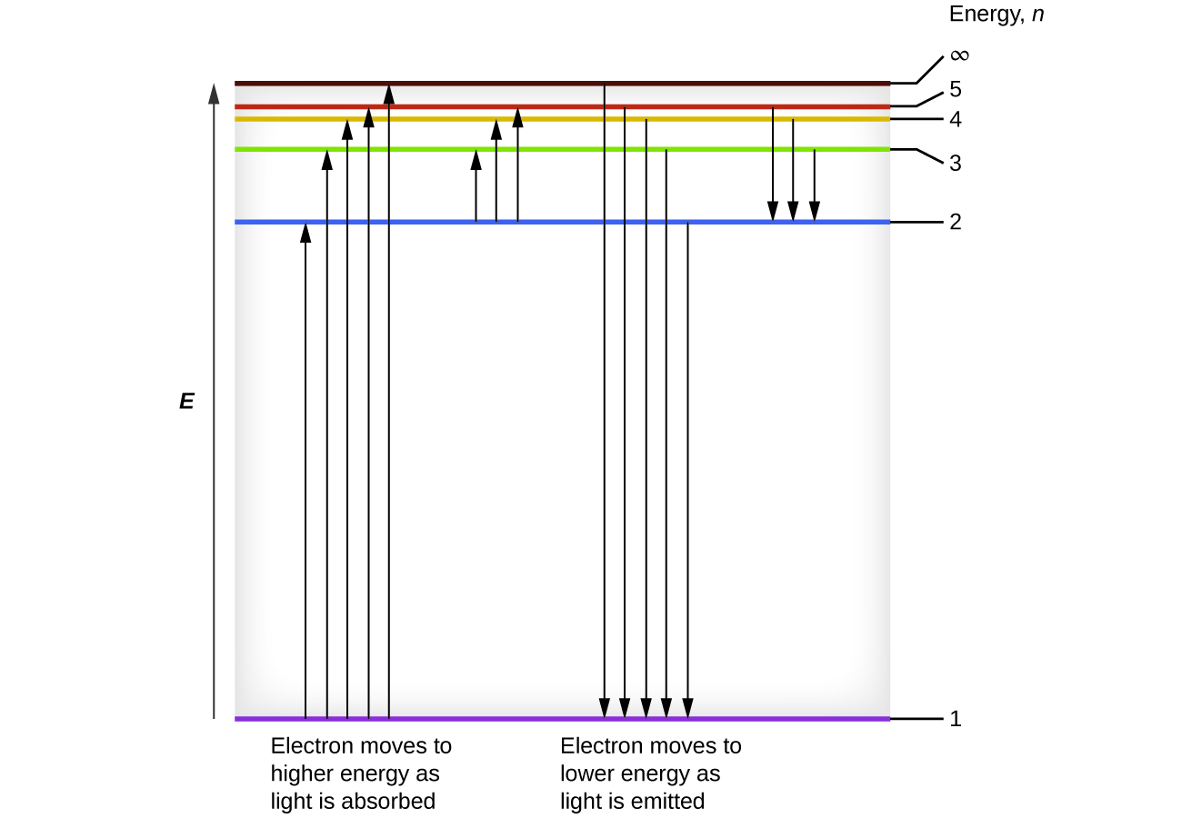
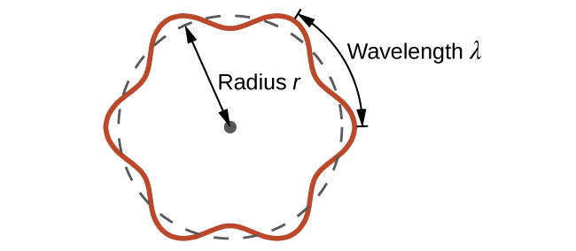
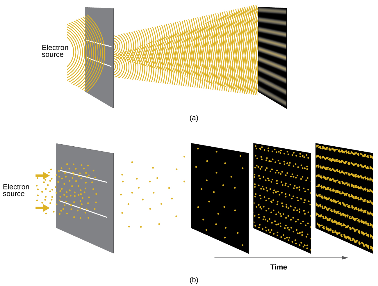
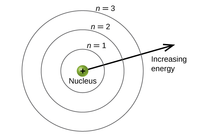
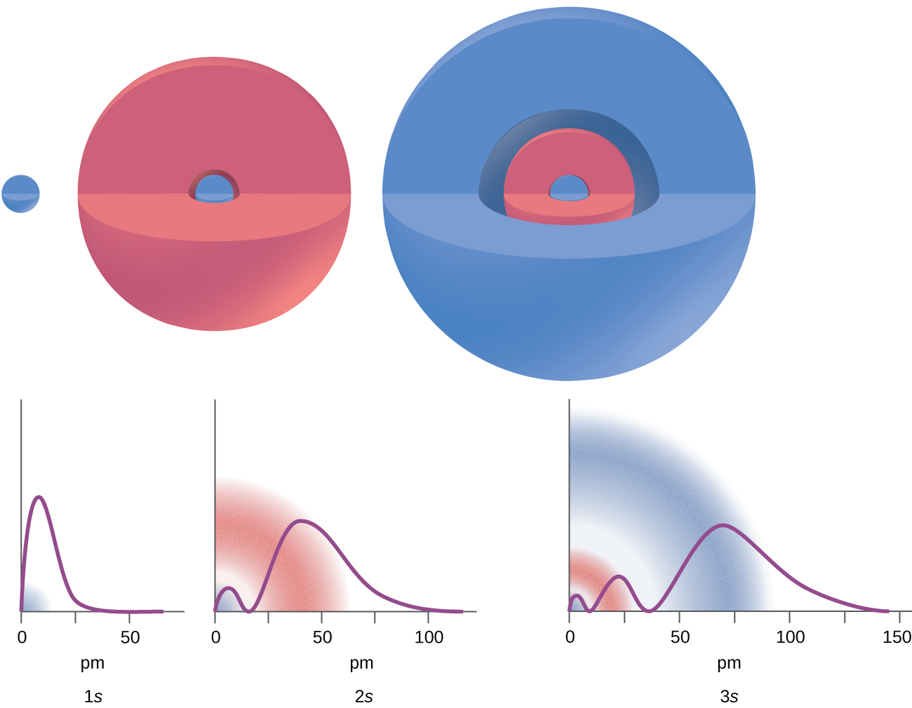
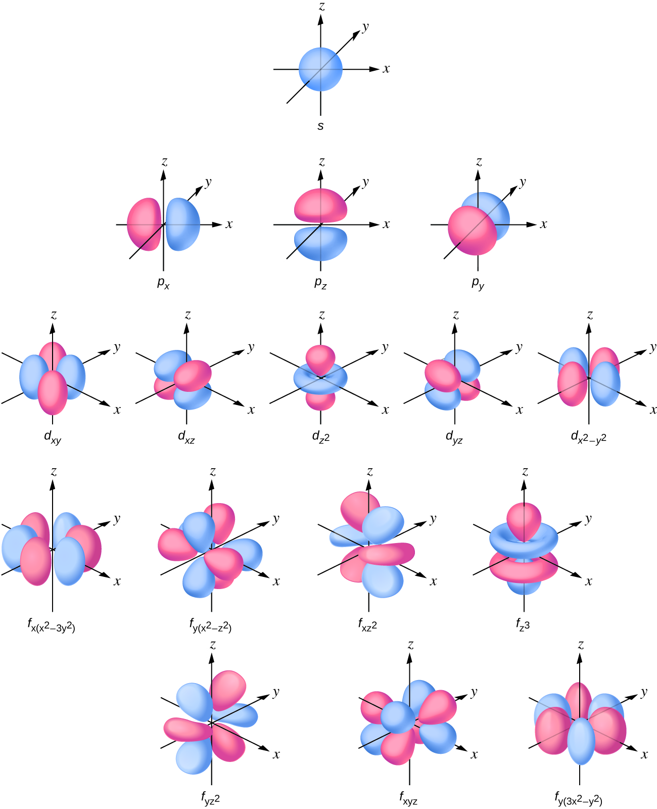
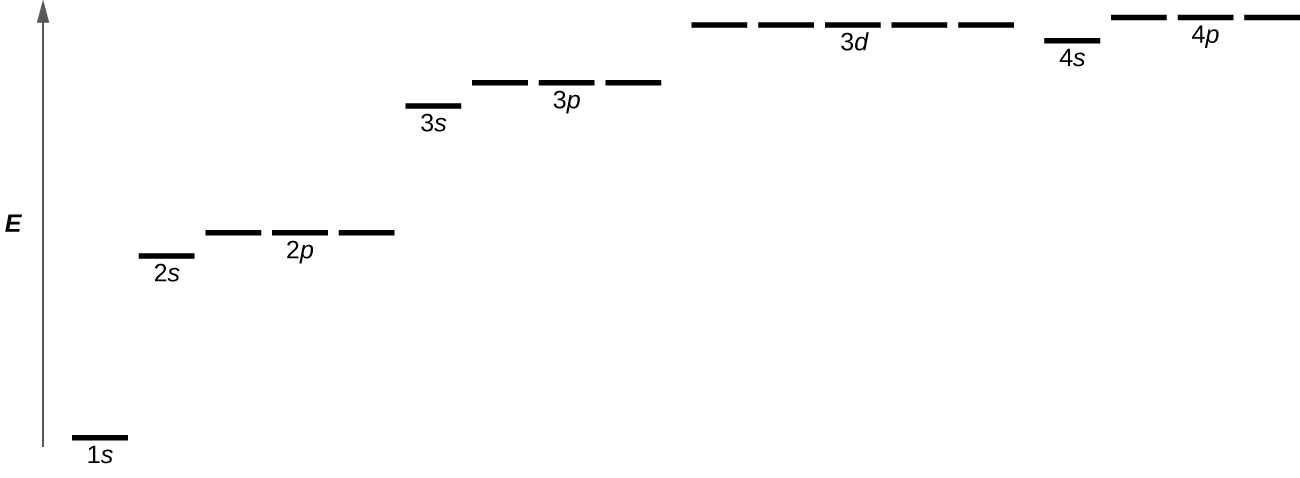
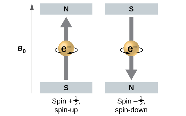
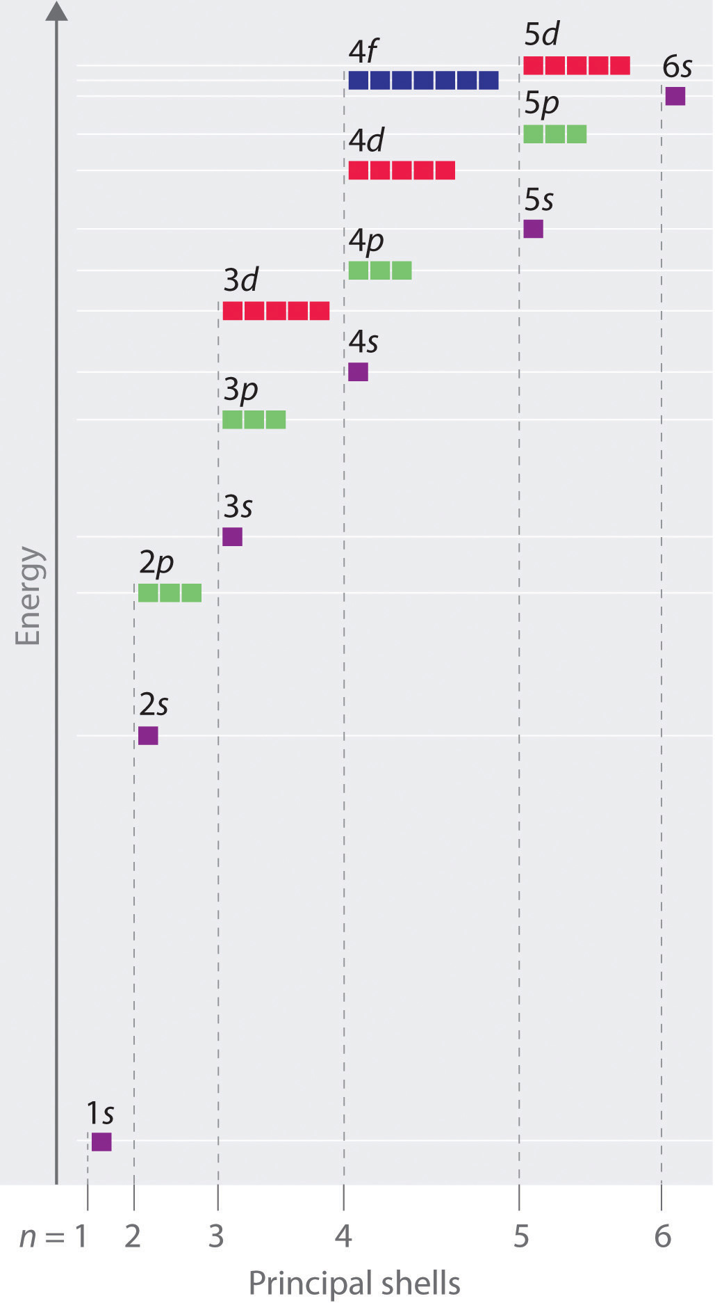

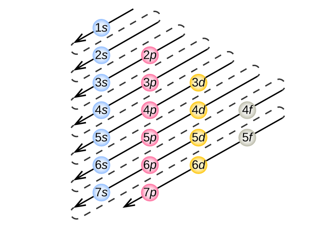
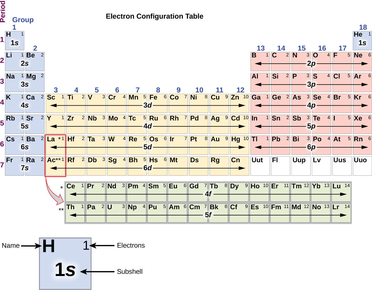


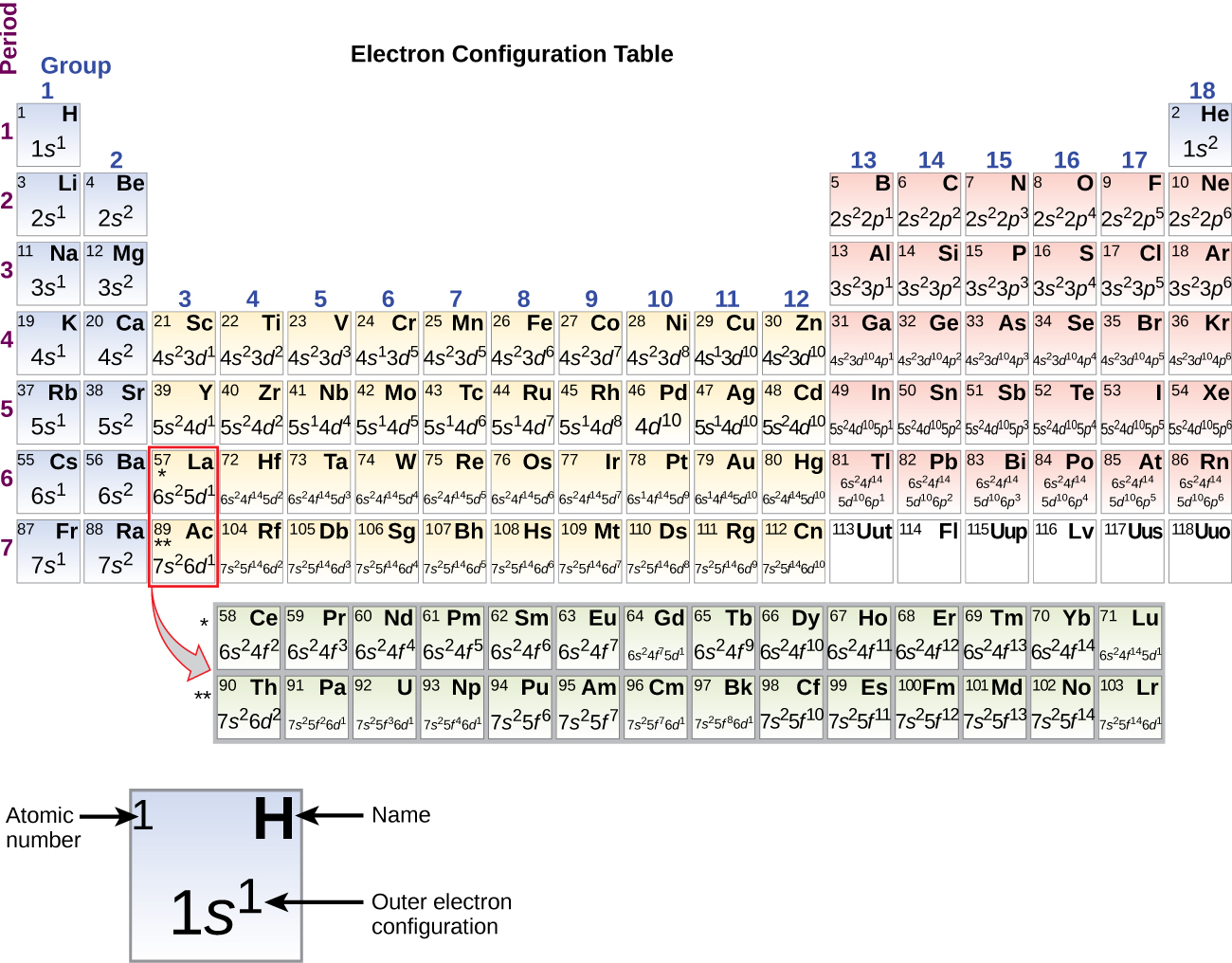


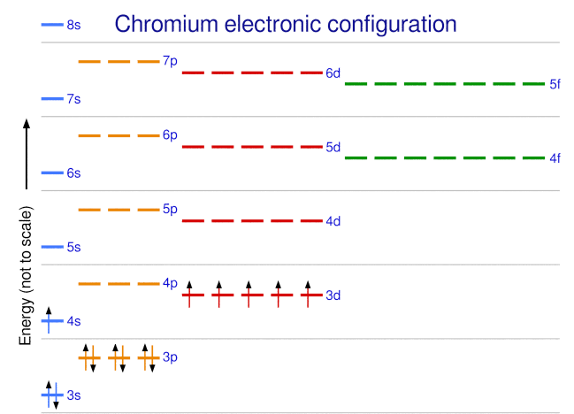
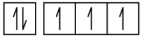
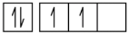
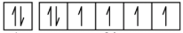
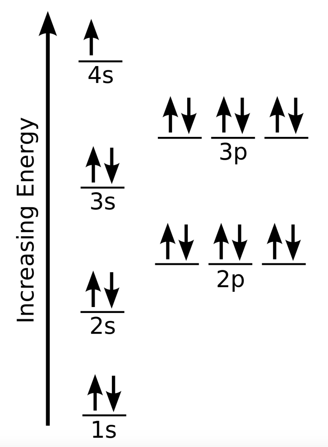
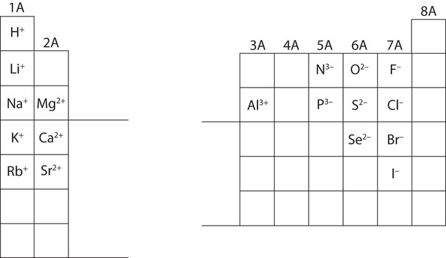
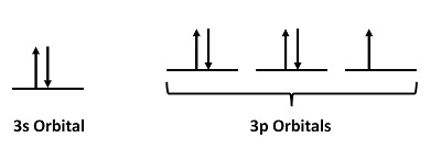

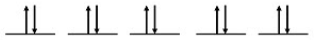

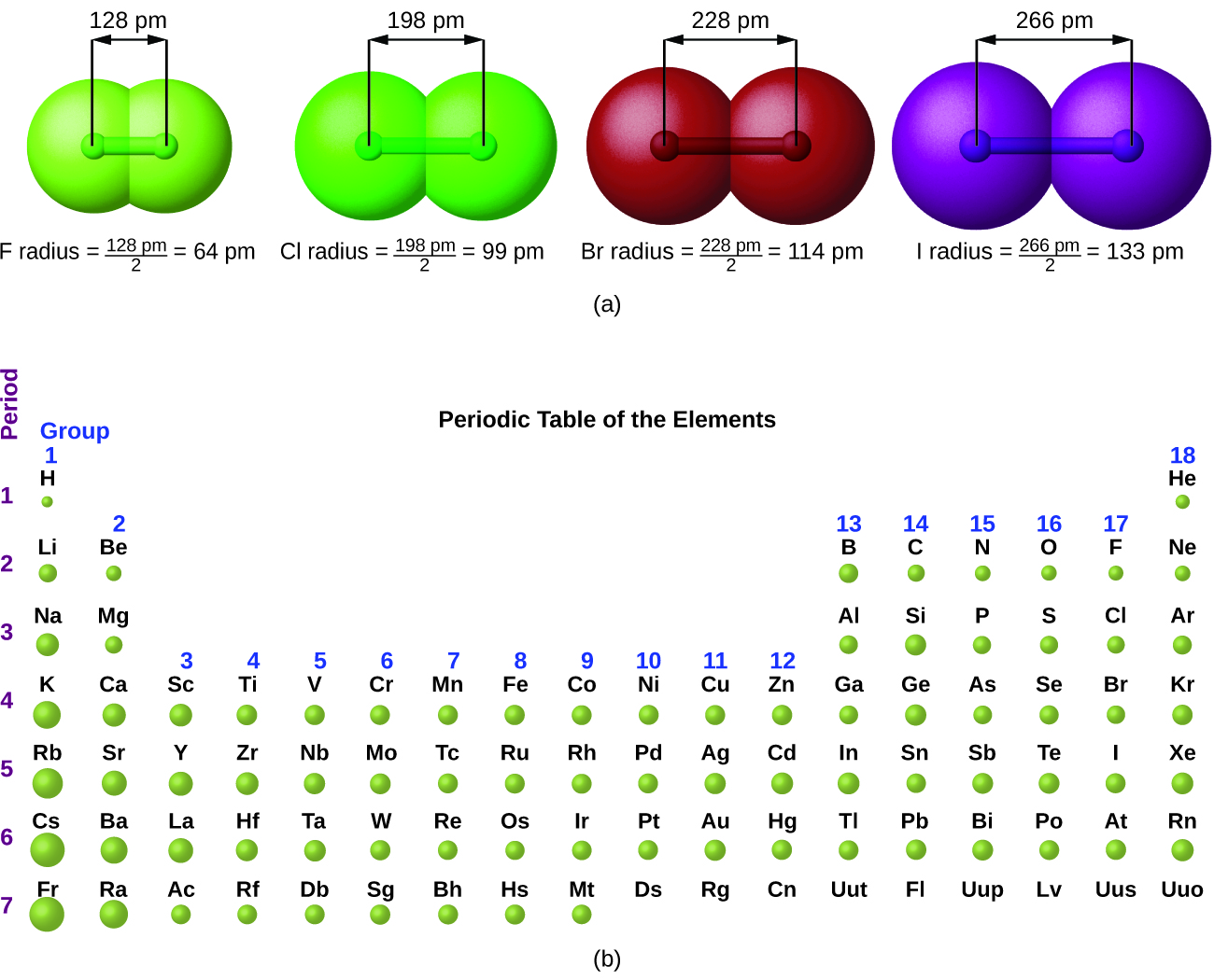
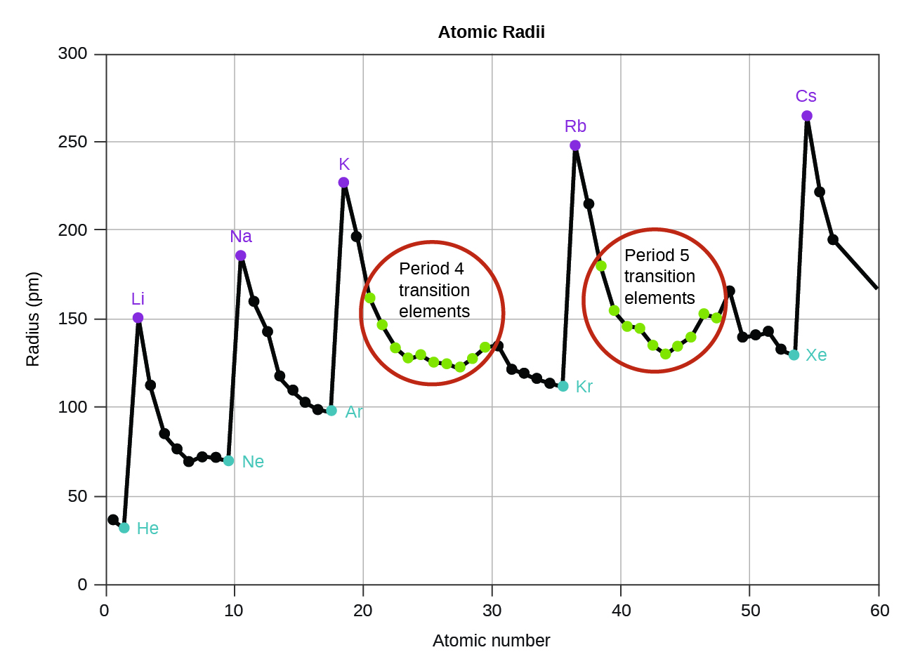

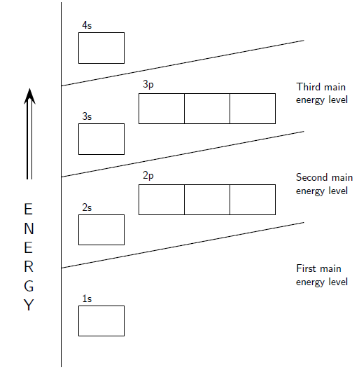
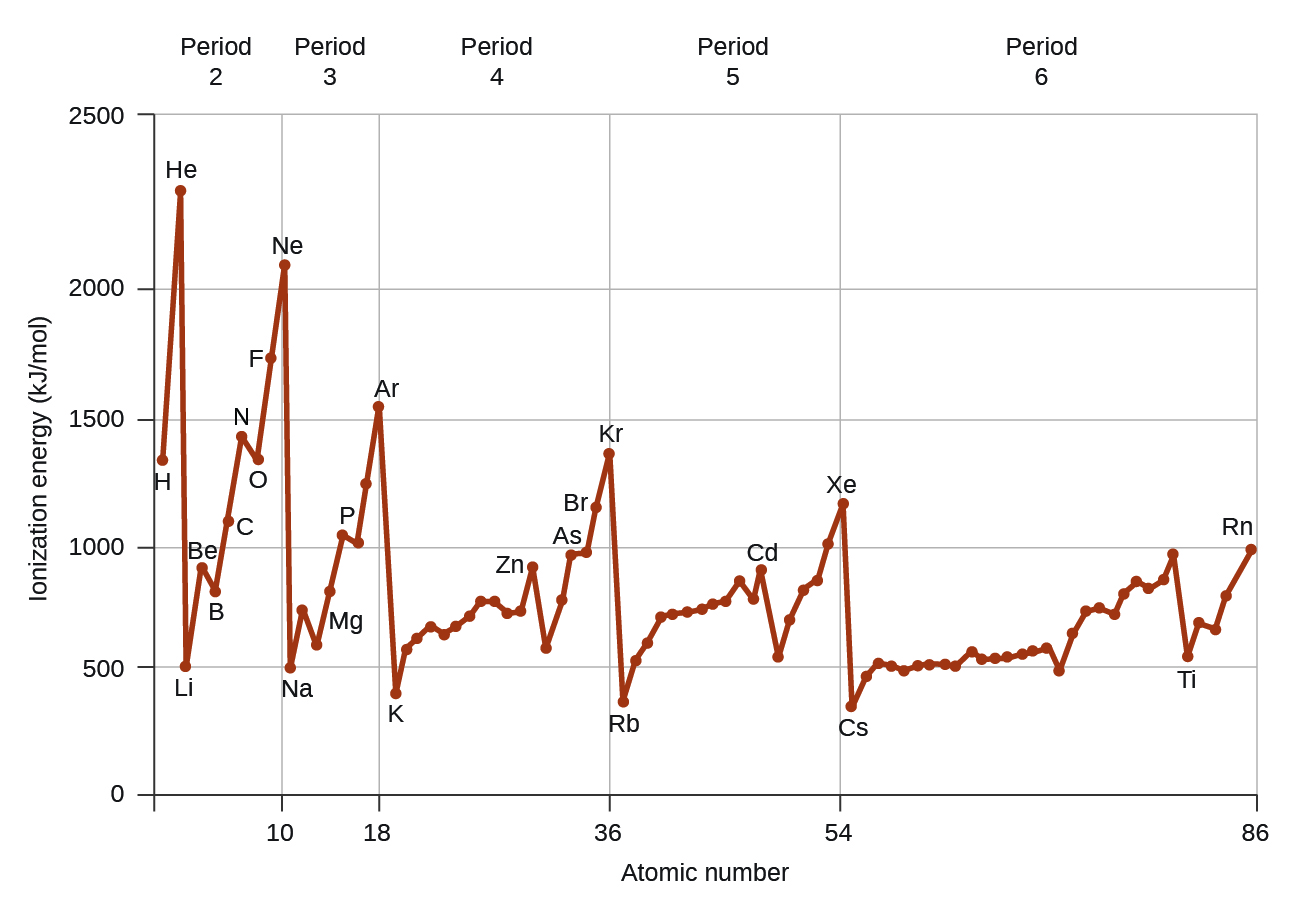
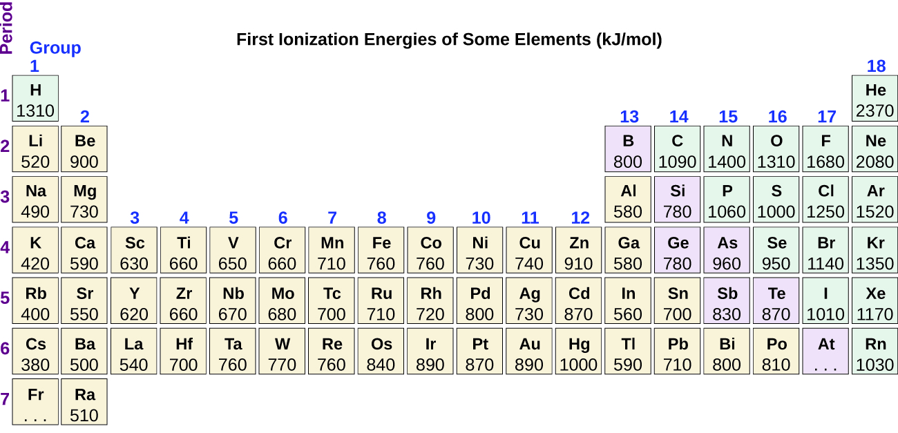
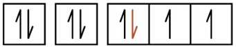
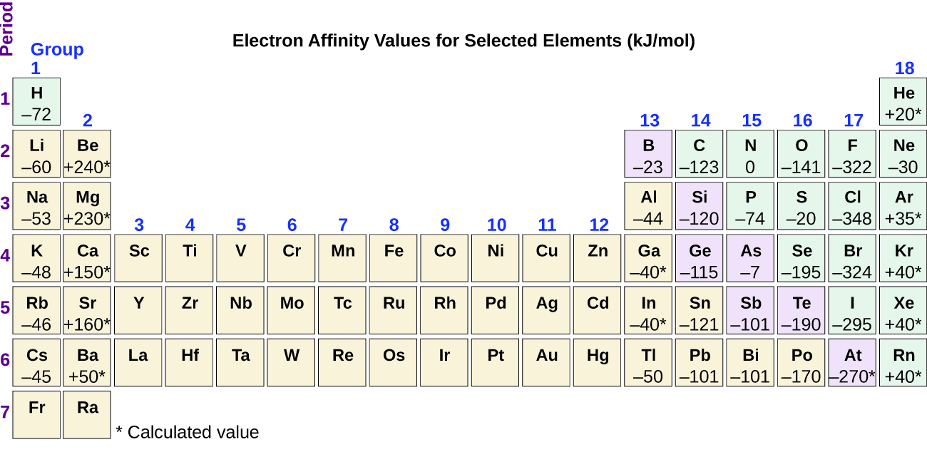
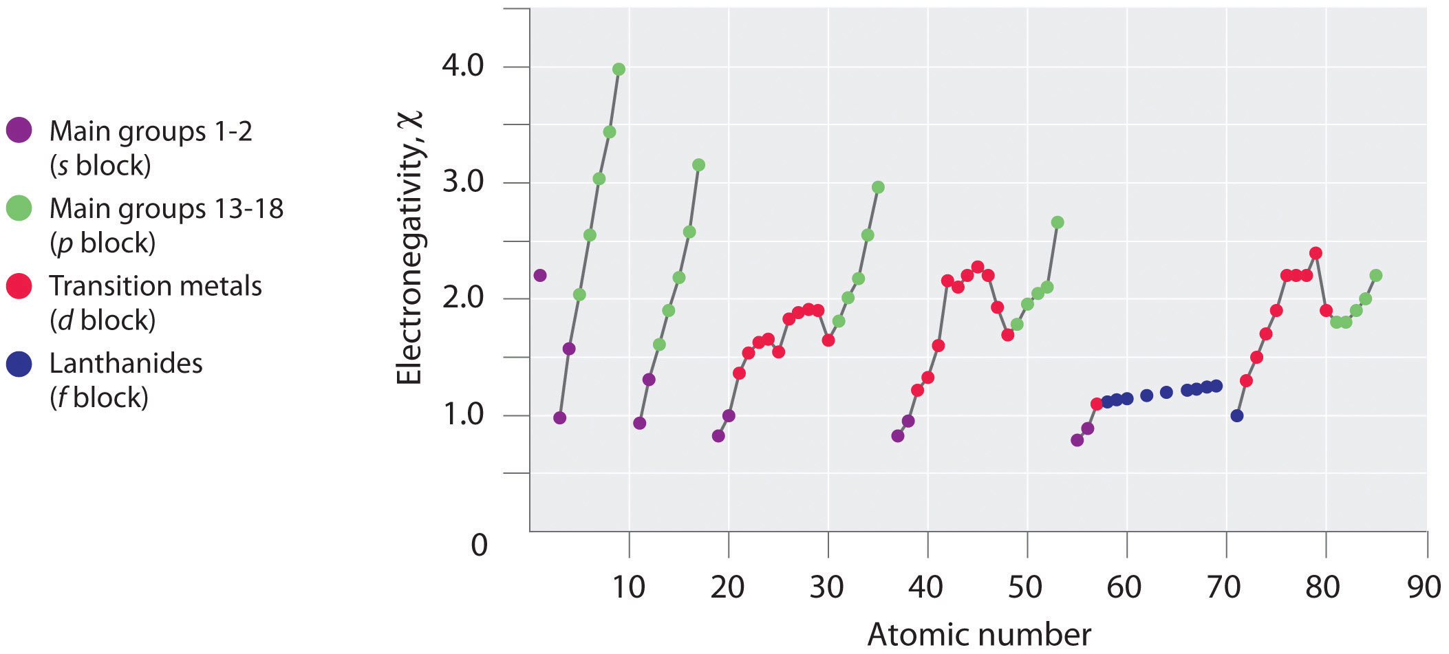
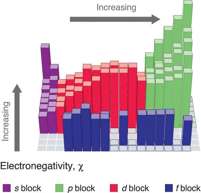
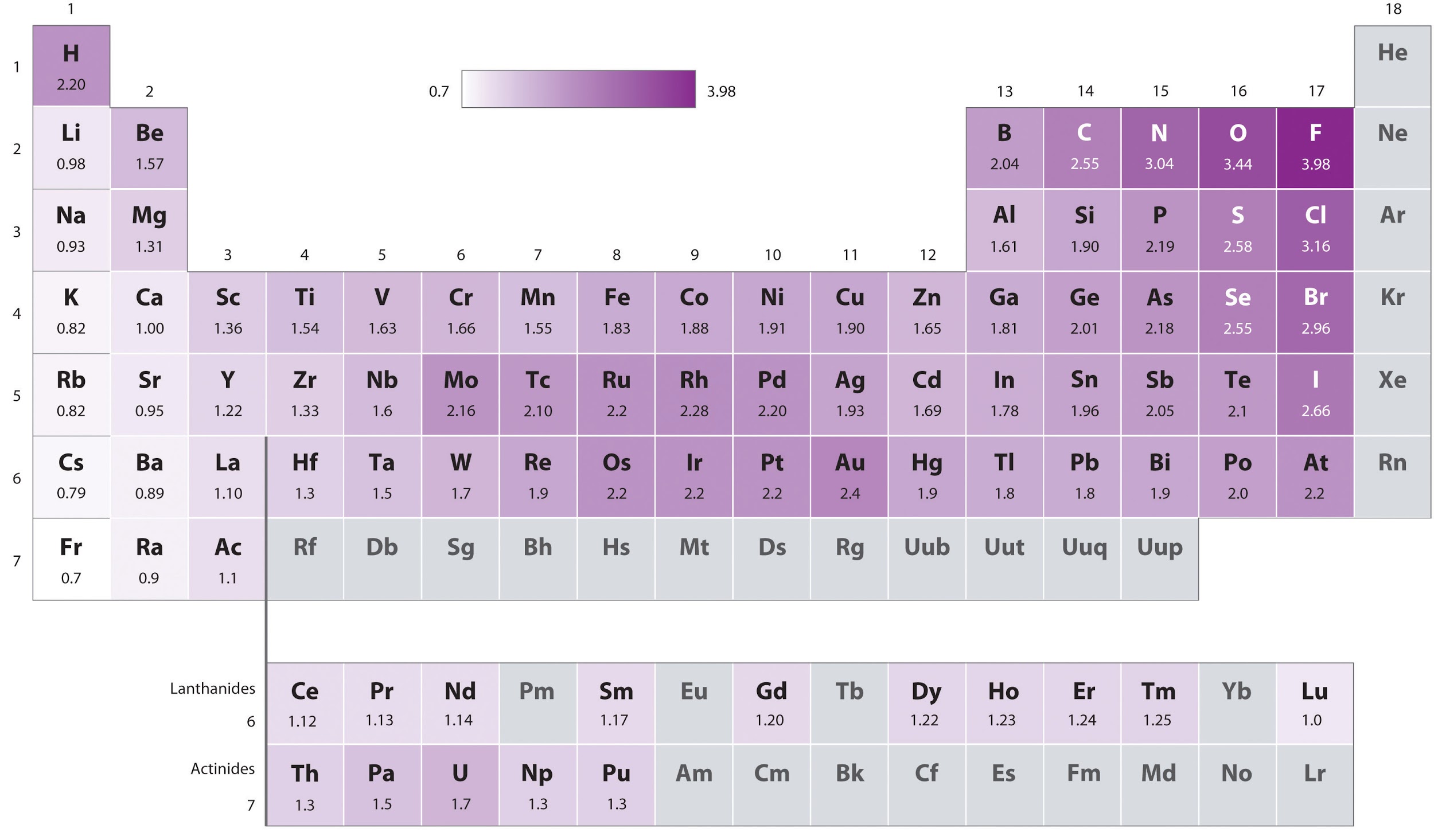


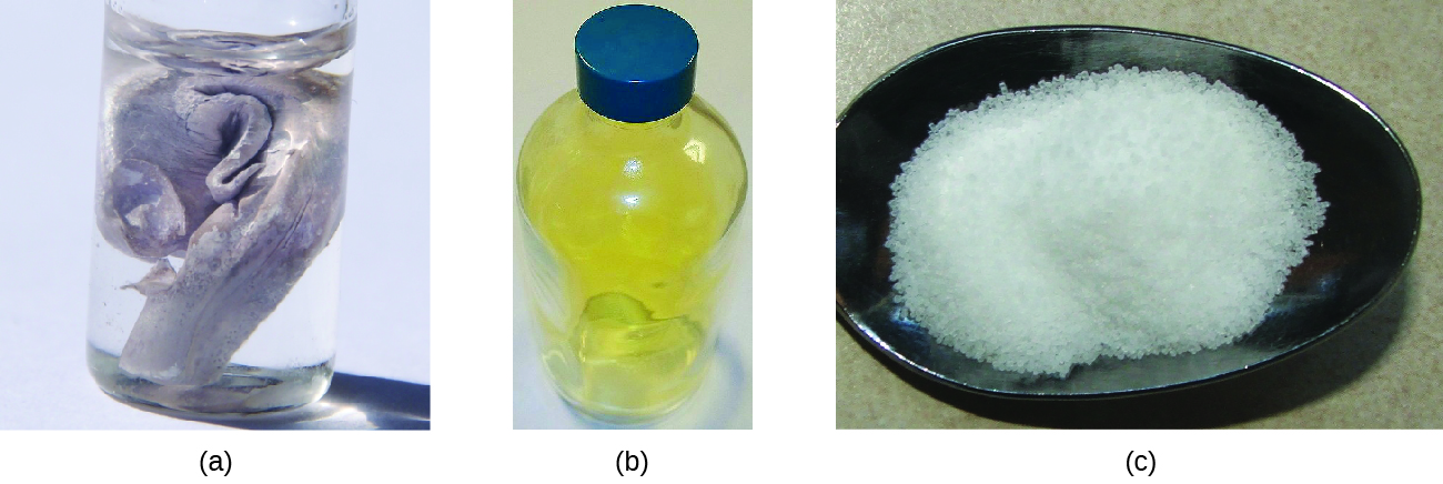
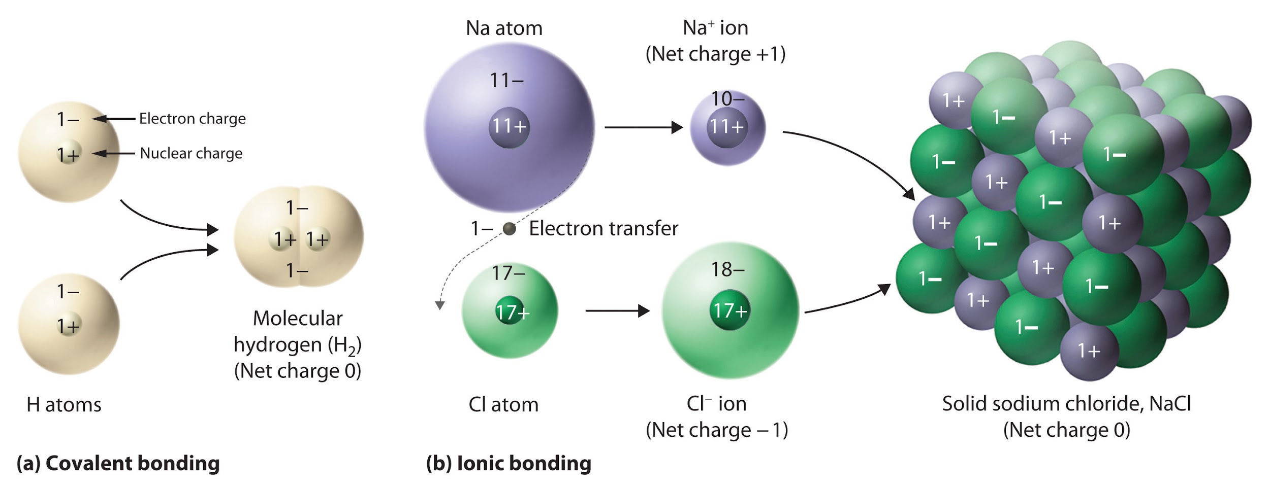
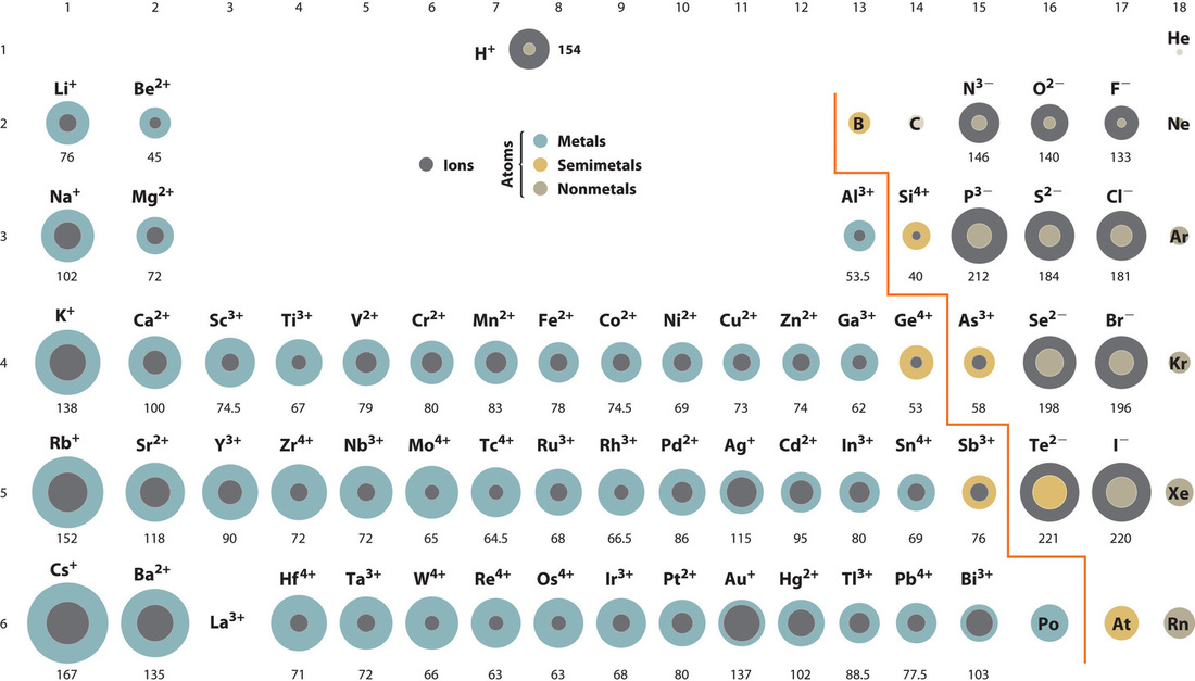
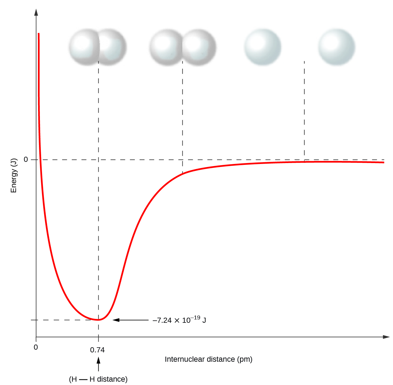
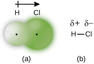
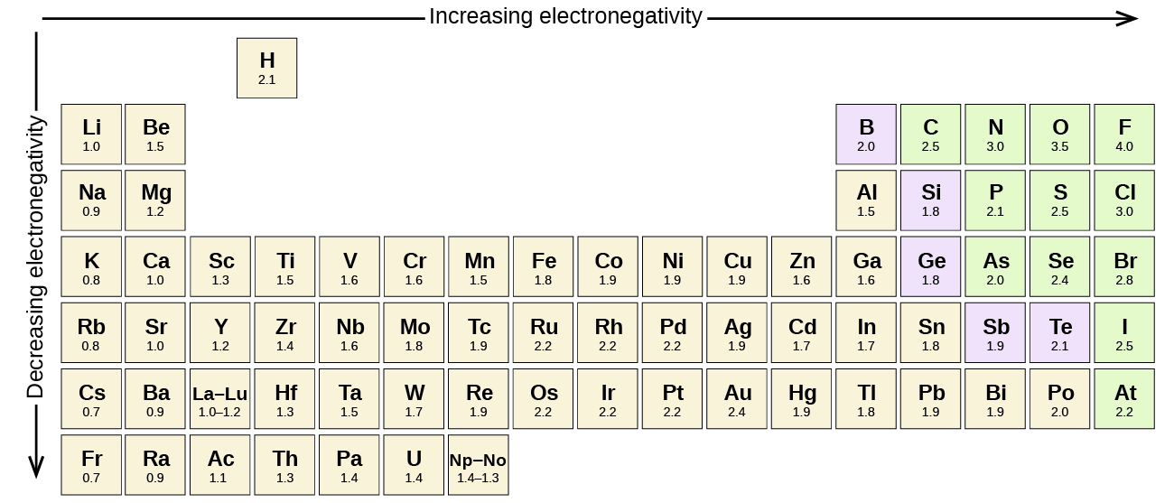
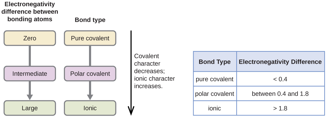

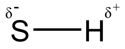
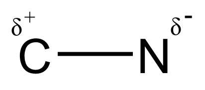
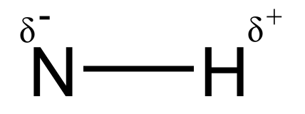
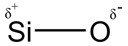

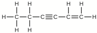

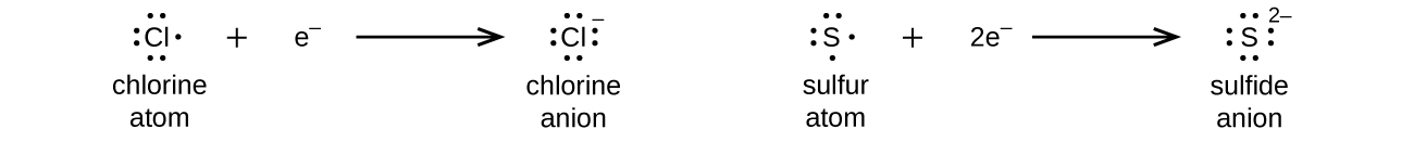
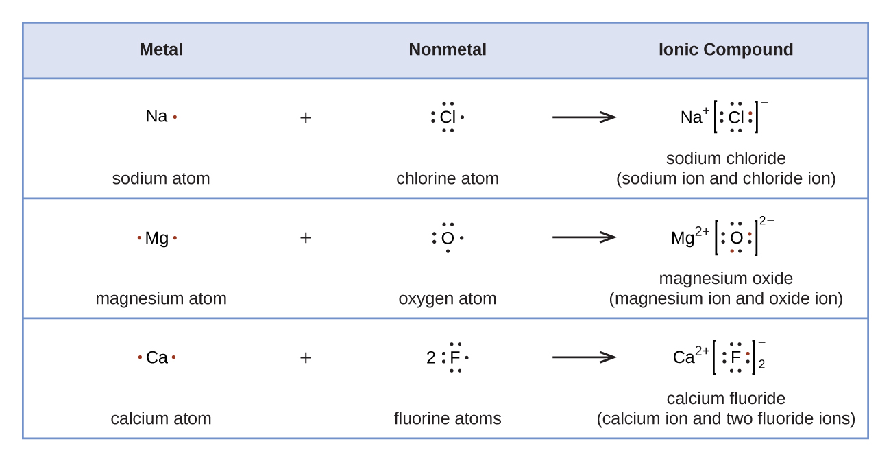
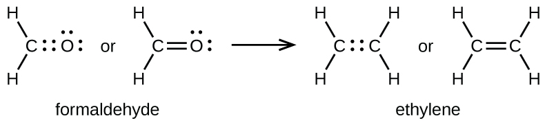
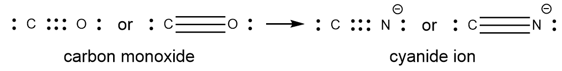 In the Lewis bonding model, we frequently describe the number of electron pairs that hold two atoms together as the
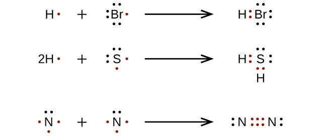
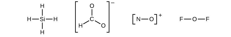
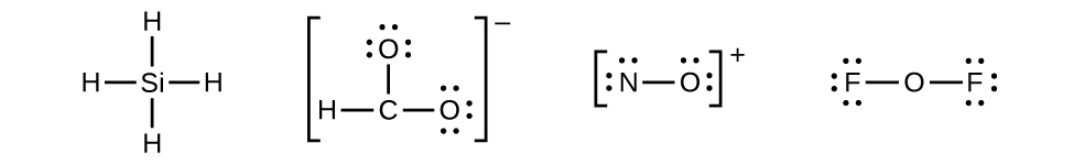
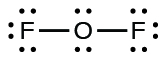

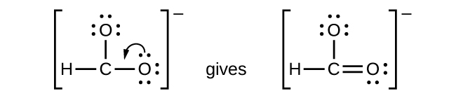

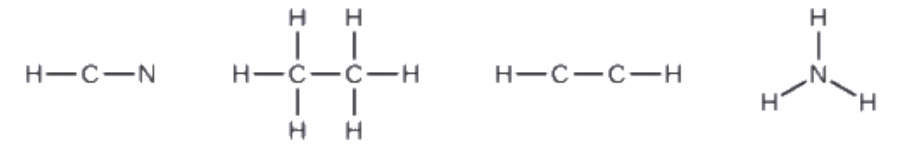
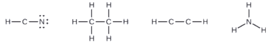
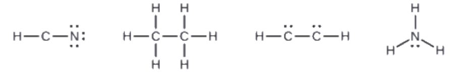
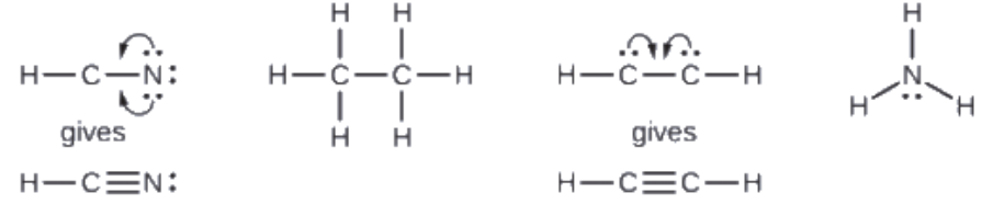

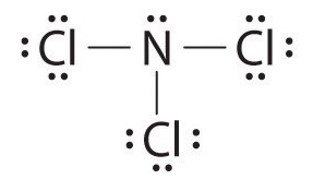


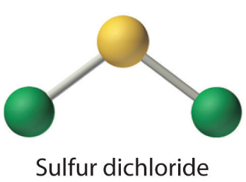
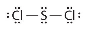
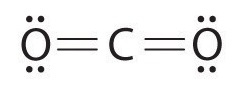
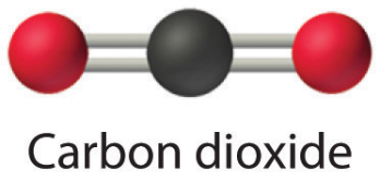
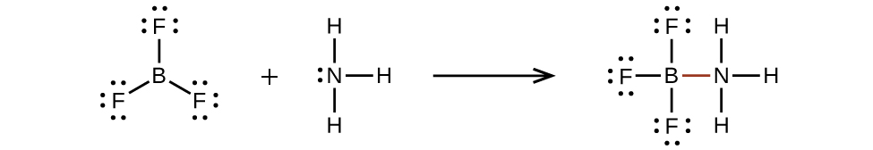

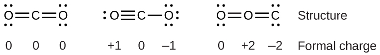
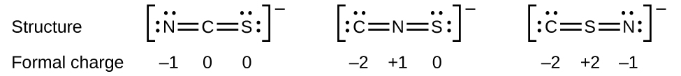
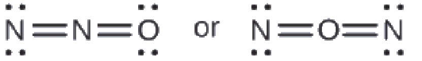
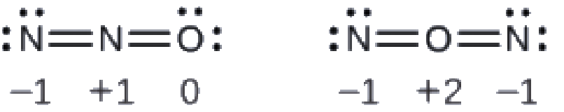

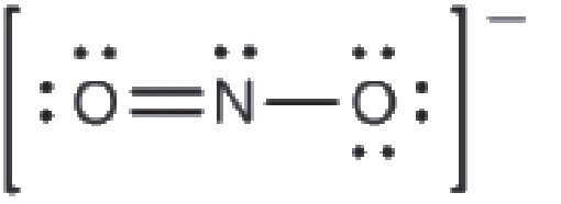
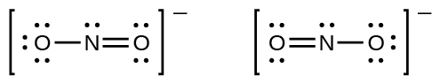
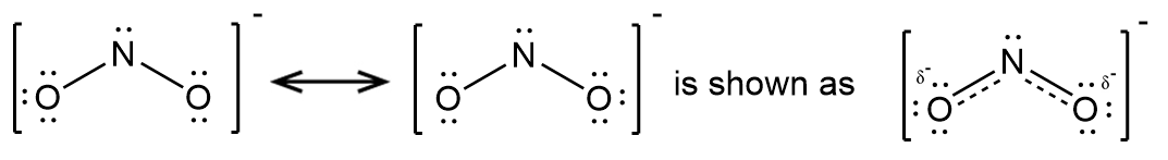
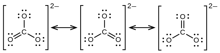
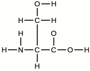
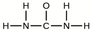
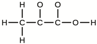
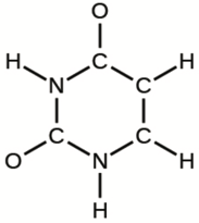


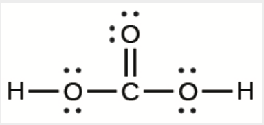
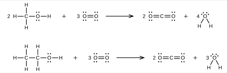
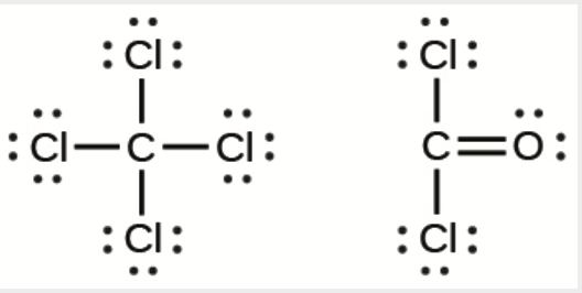
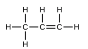
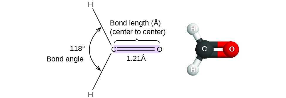


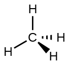
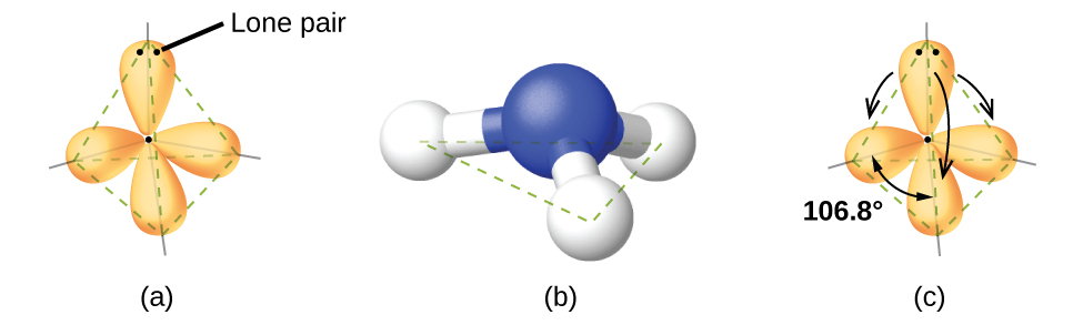
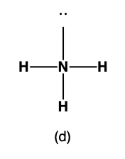
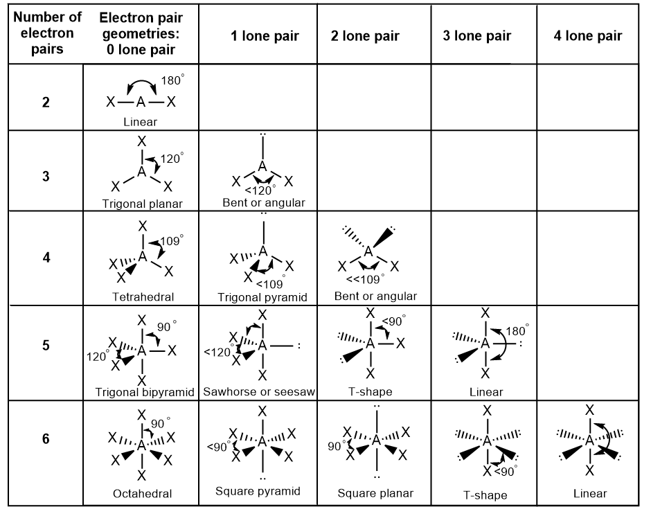
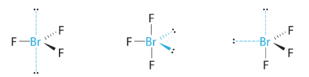
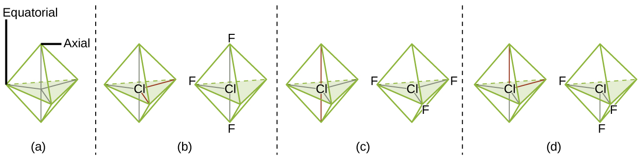
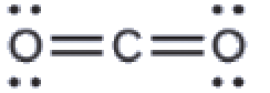
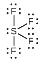
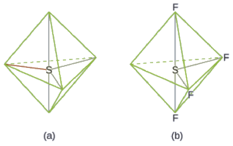
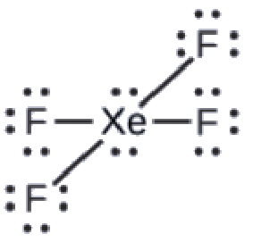
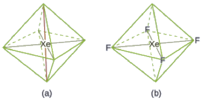
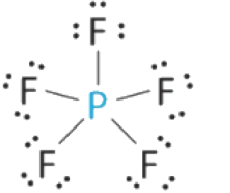
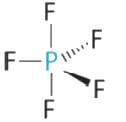
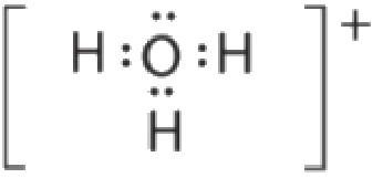
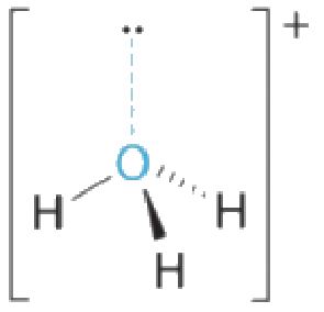
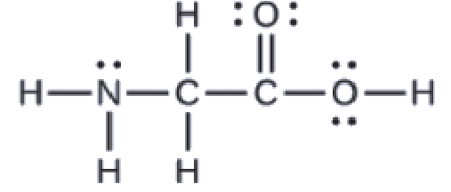
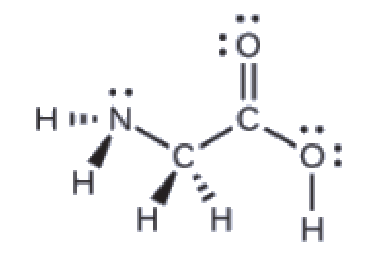
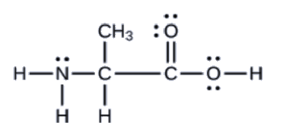
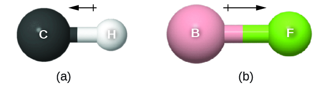
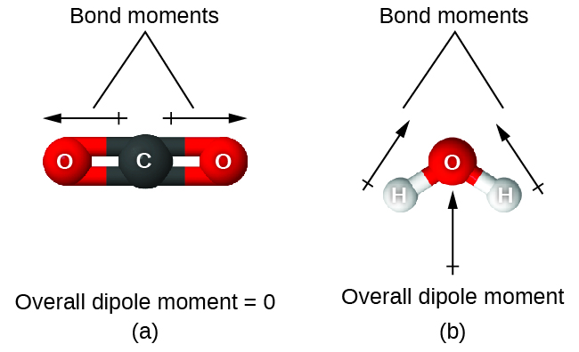
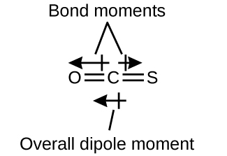
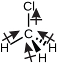

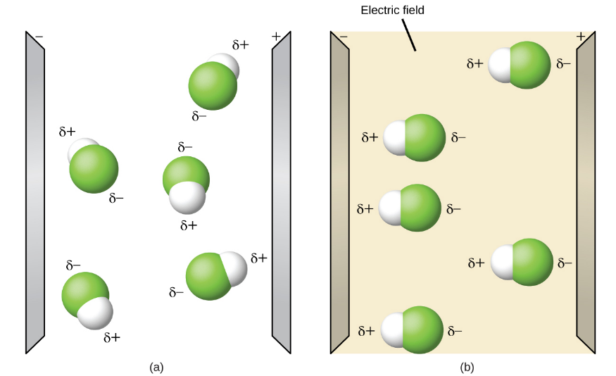
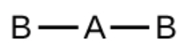
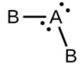
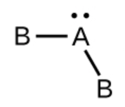
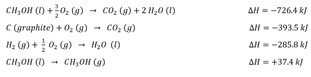
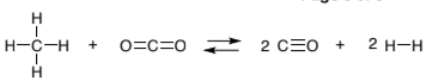
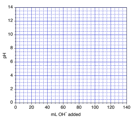
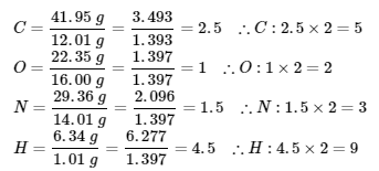
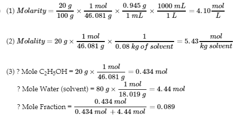
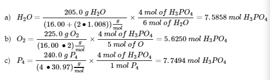
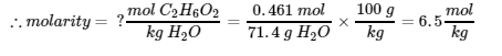
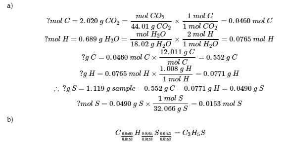
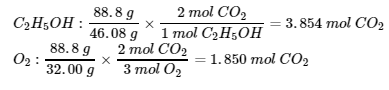
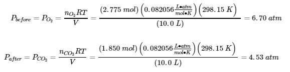
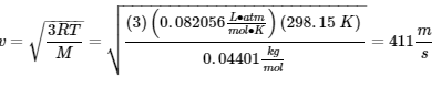
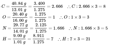
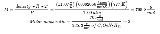
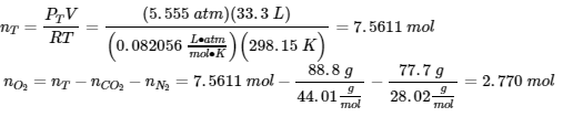
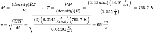
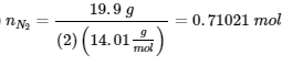
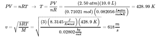
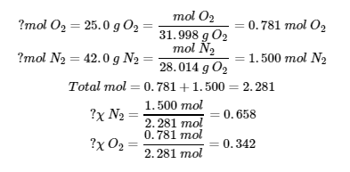
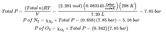
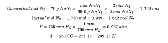
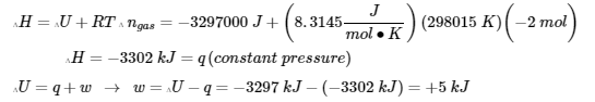
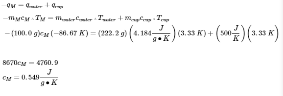
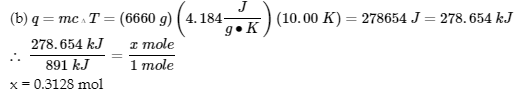
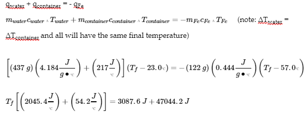
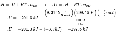
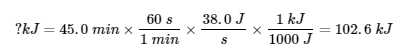
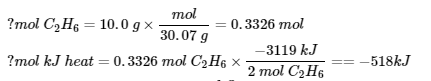
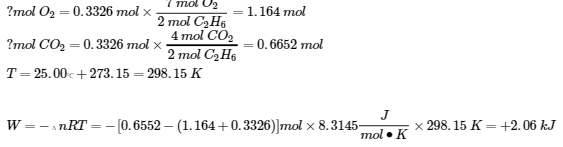
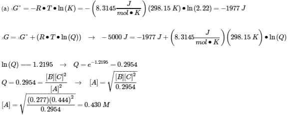
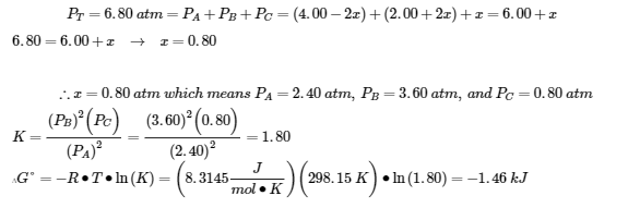
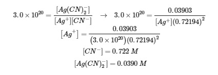
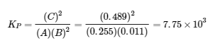
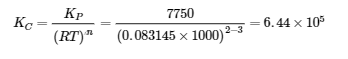
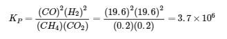
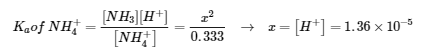
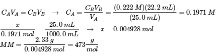
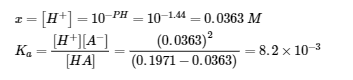
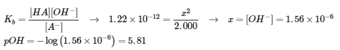

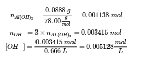 ∴ pOH = 2.29 and pH = 11.71
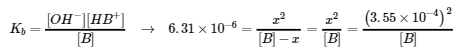
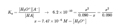
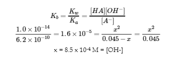
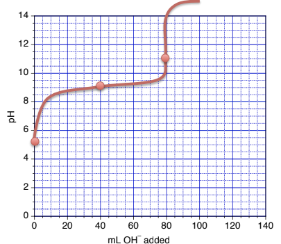
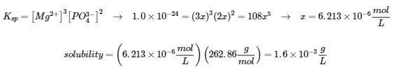
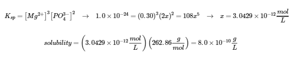
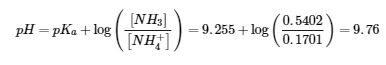
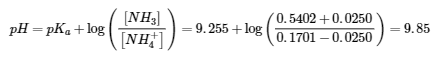
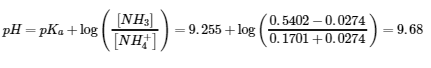
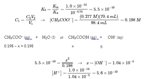
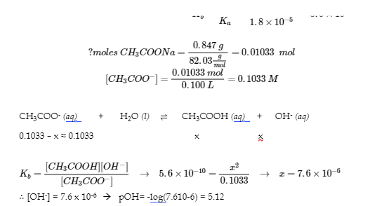
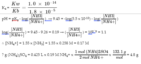
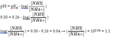
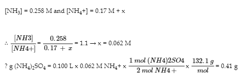
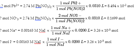
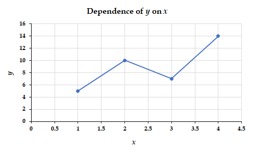
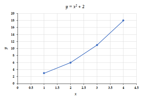


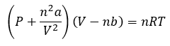
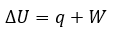
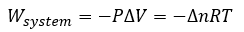
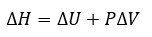
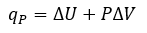


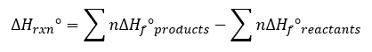
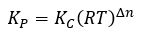
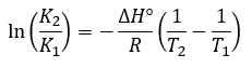
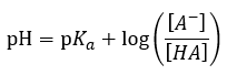
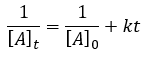
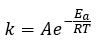
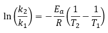


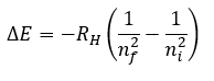
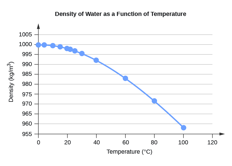
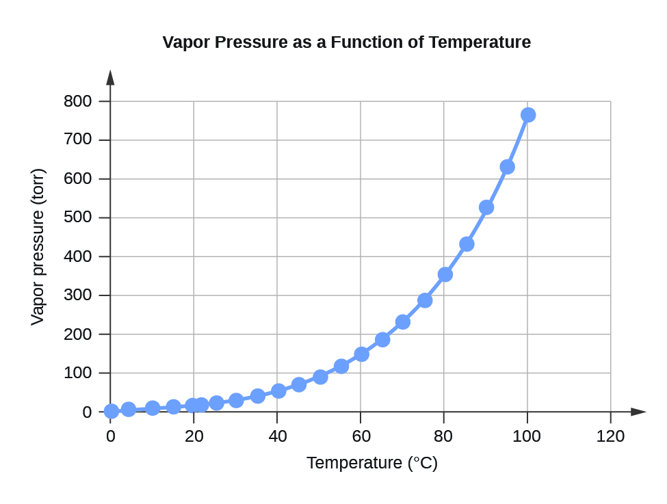
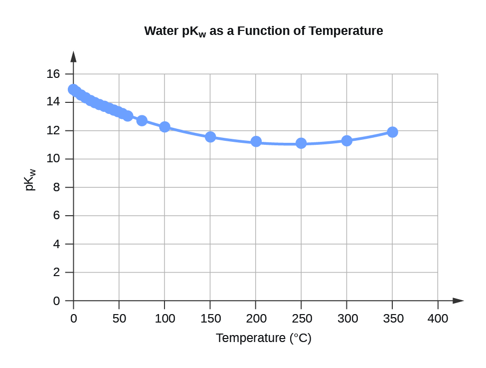 Figure F.3 Water pKW as a Function of Temperature