Key Terms
Cramer’s rule
An explicit formula for the solution of a system of linear equations with as many equations as unknowns, valid whenever the system has a unique solution.
linear circuit
An electronic circuit in which, for a sinusoidal input voltage of frequency  any steady-state output of the circuit (the current through any component, or the voltage between any two points) is also sinusoidal with frequency
load resistor
An electrical component or portion of a circuit that consumes electric power. Normally, the term “load” is used to refer specifically to the active component for which power consumption is mainly intended, as opposed to internal resistance or resistors used in conjunction with capacitors or inductors for timing.
maximum power transfer theorem
Maximum power is transferred to a load when the internal resistance equals the load resistance; for a Thévenin-equivalent circuit, this is true when the load resistance equals the Thévenin resistance.
mesh analysis
A method that is used to solve planar circuits for the currents (and indirectly the voltages) at any place in an electrical circuit.
mesh current
The currents defined in mesh analysis as flowing around each loop of a planar circuit. The actual current through each branch of the circuit is found as a combination of the mesh currents in that branch.
planar circuit (mesh)
An electrical circuit that can be drawn on a plane surface with no wires crossing each other.
superposition theorem
The response (voltage or current) in any branch of a linear circuit having more than one independent source equals the algebraic sum of the responses caused by each independent source acting alone, where all the other independent sources are replaced by short circuits.
Thévenin-equivalent circuit
A simple circuit, equivalent to any more complex linear circuit, involving the Thévenin voltage and Thévenin resistance relative to a particular load. In the Thévenin-equivalent circuit, the Thévenin voltage and resistance are connected in series with the load.
Thévenin resistance
One component of a linear circuit’s Thévenin-equivalent, found by removing the load resistor from the original circuit and calculating the total equivalent resistance between the two load connection points.
Thévenin’s theorem
An electrical circuit theorem through which any complex linear circuit may be replaced by its Thévenin-equivalent with respect to a given load.
Thévenin voltage
One component of a linear circuit’s Thévenin-equivalent, found by removing the load resistor from the original circuit and calculating the potential difference from one load connection point to the other.
Key Equations
| Cramer’s rule |  |
| Current through a load resistor |  |
| Voltage across a load resistor |  |
| Power dissipated in a load resistor |  |
Summary
7.1 Mesh Analysis
7.2 Superposition Theorem
- Linear circuits can be analysed by calculating contributions to current for each voltage source independently
- Steps in superposition method:
- Replace all potential sources but one with a short circuit; find the voltage/current through each branch of the network.
- Repeat for each potential source.
- Add up all the separate voltages/currents in each branch.
7.3 Thévenin’s Theorem
- Any linear circuit containing several voltage sources and resistors can be simplified to an equivalent circuit with a single voltage source and resistance connected in series with a load. Specifically, the three components connected in series are:
- Load resistor,
 ;
; - Thévenin voltage
 , found by removing from the original circuit and calculating the potential difference from one load connection point to the other;
 - Thévenin resistance
 , found by removing from the original circuit and calculating the total equivalent resistance between the two load connection points.
- Once the Thévenin voltage and resistance are determined, the Thévenin-equivalent circuit is redrawn with the Thévenin voltage attached to the Thévenin resistance in series, and any load resistance attached between the two connection points
- Maximum power transfer theorem: maximum power is transferred to a load when the internal resistance equals the load resistance; for a Thévenin-equivalent circuit, this is true when the load resistance equals the Thévenin resistance
Answers to Check Your Understanding
7.1 a.
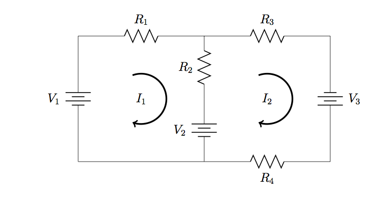
![\[\mathbf{V}=\left(\begin{array}{c}-V_1\\V_1-V_2\\V_3\end{array}\right),~~~\mathbf{R}=\left(\begin{array}{ccc}-(R_1+R_2+R_3)&R_3&0\\R_3&-(R_3+R_5)&R_5\\0&R_5&-(R_4+R_5)\end{array}\right)\]](https://openpress.usask.ca/app/uploads/quicklatex/quicklatex.com-2f881a811ee5402d4708d06c1ac92dda_l3.svg "Rendered by QuickLaTeX.com")
b.
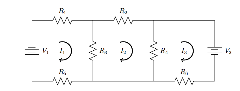
![\[\mathbf{V}=\left(\begin{array}{c}V_1-V_2\\V_2\\-V_3\end{array}\right),~~~\mathbf{R}=\left(\begin{array}{ccc}-(R_1+R_4)&0&R_4\\0&-(R_2+R_3)&0\\R_4&0&-(R_4+R_5+R_6)\end{array}\right)\]](https://openpress.usask.ca/app/uploads/quicklatex/quicklatex.com-4fa6b1daf1ad899ab1ca4ad9f78a3d3d_l3.svg "Rendered by QuickLaTeX.com")
c.
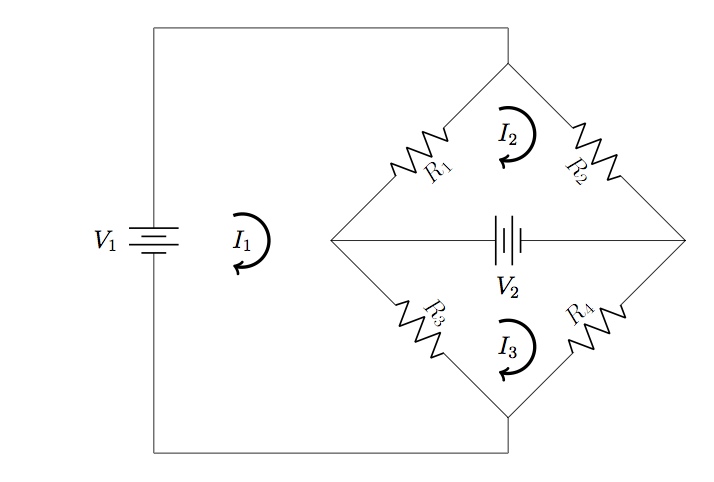
![\[\mathbf{V}=\left(\begin{array}{c}-V\\0\\0\end{array}\right),~~~\mathbf{R}=\left(\begin{array}{ccc}-(R_1+R_4)&R_1&R_4\\R_1&-(R_1+R_2+R_3)&R_3\\R_4&R_3&-(R_3+R_4+R_5)\end{array}\right)\]](https://openpress.usask.ca/app/uploads/quicklatex/quicklatex.com-a220d95df06bb084c42e0cc8fb011fe5_l3.svg "Rendered by QuickLaTeX.com")
7.2 Replacing the  source with a short means current from the
  source passes through the short. With the source replaced with a short, the current through the
  resistor due to the source is
![\[I_{7\Omega}=\frac{6.00~\mathrm{V}}{7.00~\Omega}=\frac{6.00}{7.00}~\mathrm{A}.\]](https://openpress.usask.ca/app/uploads/quicklatex/quicklatex.com-2d1113369963e8a3beb40643f4a5ec99_l3.svg "Rendered by QuickLaTeX.com")
Therefore, the current through the resistor is  and the power dissipated is
  In fact, since the
  -resistor is connected directly to the terminals of the source, the current is
  regardless of the value of the battery.
7.3.  ,
,  .
.
Conceptual Questions
7.1 Mesh Analysis
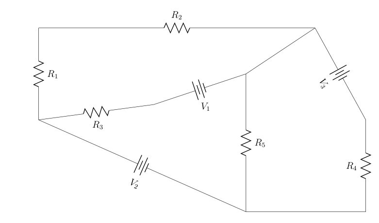
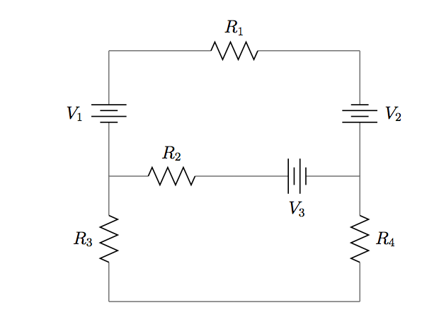
1 Sally and Frank are asked to find the  and
and  matrices for the circuit below. They both follow the procedure for reading off matrix elements described in Mesh Analysis. When comparing results, they find that they have the same elements in the first rows of both and , but the elements in the second and third rows of their matrices are swapped. How did this happen? Did one of them make an error? If given values for the voltages and resistances, should they expect to find the same currents through each component? Explain.
7.2 Superposition Theorem
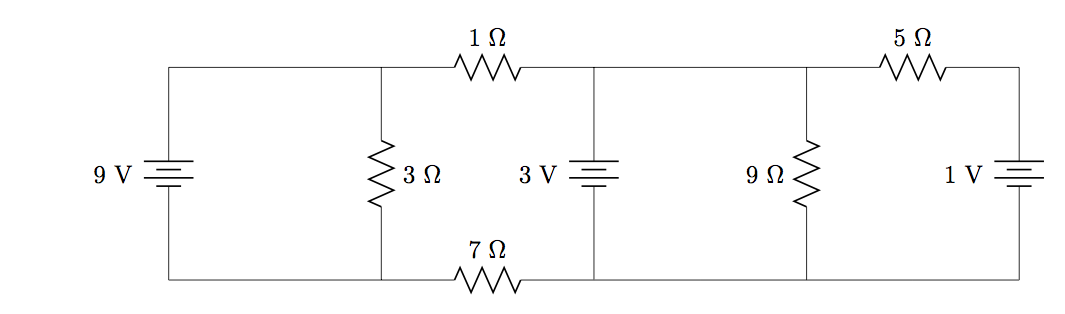
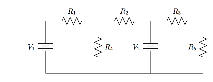
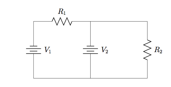
2. How much power is used by the  -resistor in the circuit below? How much power is used by the
  -resistor? Explain why the answers are obvious, with no need to do any work. (Hint: this problem is best approached using superposition method).
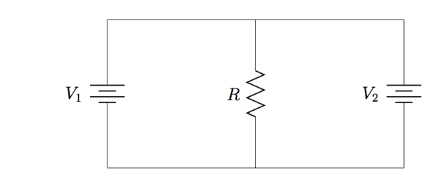
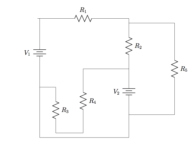
3. (a) Use superposition theorem to determine the potential difference across the resistor in the circuit below. (b) Explain why mesh analysis is a bad approach to use for this problem (e.g. you could demonstrate this by applying the mesh strategy and Cramer’s rule to calculate mesh currents and interpret the result).
7.3 Thévenin’s Theorem
4. Efficiency. The efficiency of a circuit is defined as the ratio between the power used by a load and the total power used. (a) Show that the general expression for efficiency can be written as
![\[\eta=\frac{R_L}{R_{\mathrm{th}}+R_L}.\]](https://openpress.usask.ca/app/uploads/quicklatex/quicklatex.com-3c136b49bd1cf5c2e036bf653216306a_l3.svg "Rendered by QuickLaTeX.com")
For any given and , show that: (b) the condition for minimum efficiency ( ) corresponds to maximum current, but the voltage across and power dissipated at the load are both small; (c) the condition for maximum efficiency () corresponds to maximum voltage across the load, but current through and power dissipated at the load are both small; (d) the condition of maximum power transfer (
 ), while only moderately efficient, corresponds to both moderate voltage across and moderate current through the load. (Hint: You may find it useful to refer to Equations 7.3.1-7.3.3).
Problems
7.1 Mesh Analysis
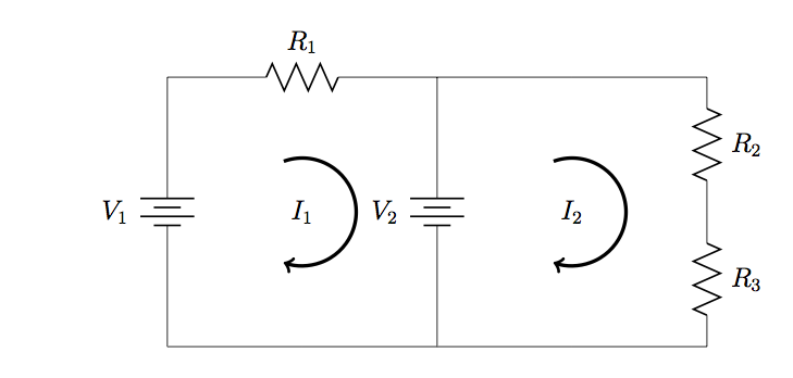
5. Apply Cramer’s rule to find expressions for  and
and  in terms of the given resistances and voltages.
6. Refer to the circuit in Problem 5, with  ,
,  ,
,  ,
,  , and
, and  . Apply Cramer’s rule to calculate the values of and .
7. Apply Cramer’s rule to find expressions for and in terms of the given resistances and voltages.
8. Refer to the circuit in Problem 7, with , ,  ,
,  ,
,  ,
,  , and
, and  . Apply Cramer’s rule to calculate the values of and .
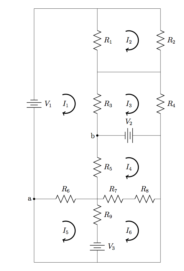
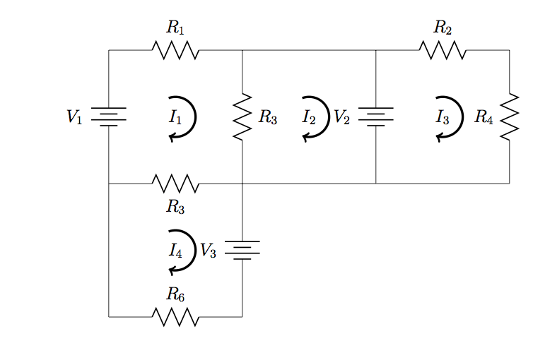
9. Apply Cramer’s rule to find expressions for , , and  in terms of the given resistances and voltages.
10. Refer to the circuit in Problem 9, with , , , , ,  ,
,  , and
, and  . Apply Cramer’s rule to calculate the values of , , and .
11. Apply Cramer’s rule to find expressions for , , and in terms of the given resistances and voltages.
12. Refer to the circuit in Problem 11, with , , , , , and . Apply Cramer’s rule to calculate the values of , , and .
13. Find expressions for the total power supplied by all voltage sources and the total power dissipated at all resistors, and confirm that these are equal.
14. Refer to the circuit in Problem 13, with , , , , and . Calculate the total power supplied by all voltage sources and the total power dissipated at all resistors, and confirm that the two values are equal.
15. Find expressions for the total power supplied by all voltage sources and the total power dissipated at all resistors, and confirm that these are equal.
16. Refer to the circuit in Problem 15, with , ,  , , , , and . Calculate the total power supplied by all voltage sources and the total power dissipated at all resistors, and confirm that the two values are equal.
17. Find expressions for the total power supplied by all voltage sources and the total power dissipated at all resistors, and confirm that these are equal.
18. Refer to the circuit in Problem 17, with , , , , , , and . Calculate the total power supplied by all voltage sources and the total power dissipated at all resistors, and confirm that the two values are equal.
19. Find expressions for the total power supplied by all voltage sources and the total power dissipated at all resistors, and confirm that these are equal.
20. Refer to the circuit in Problem 19, with , , , , , , and . Calculate the total power supplied by all voltage sources and the total power dissipated at all resistors, and confirm that the two values are equal.
21. Find expressions for the current through and power dissipated at  in terms of the given resistances and voltages.

22. Refer to the circuit in Problem 21. Calculate (a) the mesh current values and (b) the power supplied by each voltage source, when , , , , , , , and  .
.
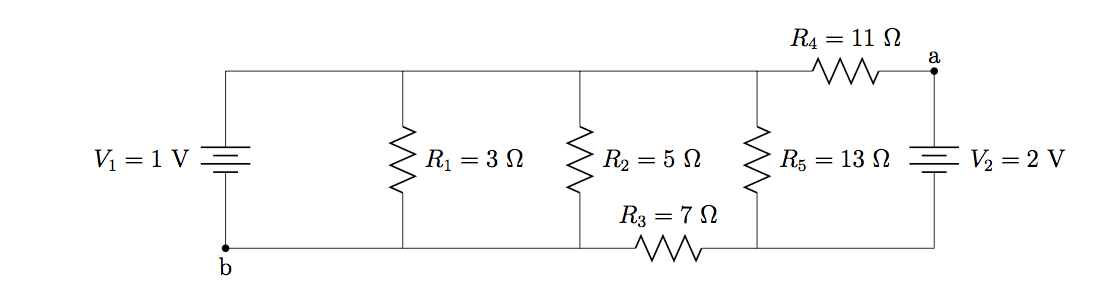
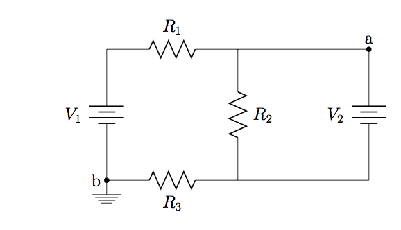
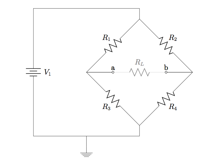
23. Find the potential difference  between points
  and
and  in the following circuit diagram.
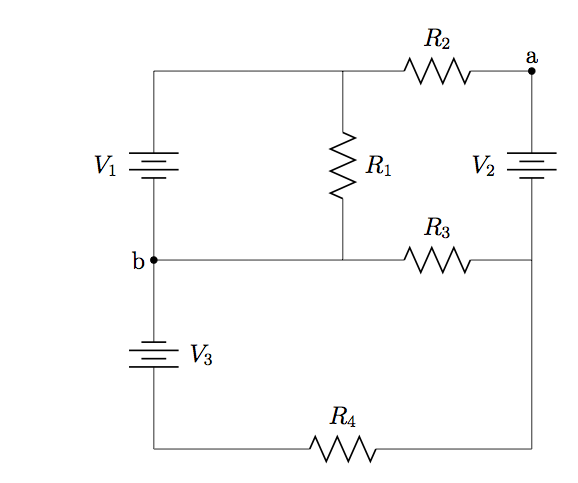
24. (a) Use a computer to calculate the mesh currents  in the following circuit diagram, when , , , , , , , ,
  ,
,  ,
,  , and
, and  . (b) Calculate the potential difference across and
  , confirming that
  .
.
7.2 Superposition Theorem
25. Use superposition method to find an expression for the current through and power dissipated by  in the circuit below.
26. Use superposition method to calculate the current through and power dissipated by in the circuit from problem 25, when , , , and .
27. Use superposition method to find expressions for (a) the currents through each resistor in the circuit below, and (b) the potential difference between points and .
28. Refer to the circuit in problem 27, with , , , , and . Use superposition method to calculate (a) the current through each resistor, and (b) the potential difference between points and .
29. Use superposition method to find an expression for the current through and power dissipated by  in the circuit below.
30. Use superposition method to determine the current through and power dissipated by in the circuit from problem 29, when , , , , , , and .
31. Use superposition method to find expressions for (a) the current through each resistor in the circuit from Problem 29, and (b) the potential difference between points and .
32. Refer to the circuit in problem 29, with, , , , , , and . Use superposition method to calculate (a) the current through each resistor, and (b) the potential difference between points and .
7.3 Thévenin’s Theorem
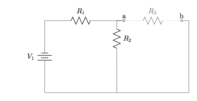
33. Find expressions for and with respect to in the circuit diagram below.
34. Refer to the circuit diagram in Problem 33, with ,  , and
, and  . Calculate (a) and with respect to , and (b) the maximum amount of power that can be used by .
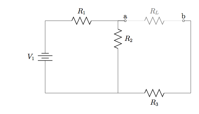
35. Find expressions for and with respect to in the circuit diagram below.
36. Refer to the circuit diagram in Problem 35, with , , , and  . Calculate (a) and with respect to , and (b) the maximum amount of power that can be used by .
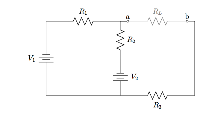
37. Find expressions for and with respect to in the circuit diagram below.
38. Refer to the circuit diagram in Problem 37, with , , , , and . Calculate (a) and with respect to , and (b) the maximum amount of power that can be used by .
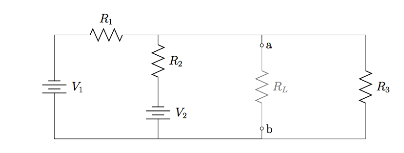
39. Find expressions for and with respect to in the circuit diagram below.
40. Refer to the circuit diagram in Problem 39, with , , , , and . Calculate (a) and with respect to , and (b) the maximum amount of power that can be used by .
41. Find expressions for and with respect to in the circuit diagram below.
42. Refer to the circuit diagram in Problem 41, with , , , and , and  . Calculate (a) and with respect to , and (b) the maximum amount of power that can be used by .
Additional Problems
43. Find the current through, and the power dissipated by  in the circuit below using (a) mesh analysis method and (b) superposition method.
44. Find the current through  and
and  in the circuit below using (a) mesh analysis method and (b) superposition method.


 . No free particle can have less charge than this, and, therefore, the charge on any object—the charge on all objects—must be an integer multiple of this amount. All macroscopic, charged objects have charge because electrons have either been added or taken away from them, resulting in a net charge.
 , and the smallest possible negative charge is
  ; these values are exactly equal. This is simply how the laws of physics in our universe turned out.
 of the mass. In addition, he showed that the negatively charged electrons perpetually orbited about this nucleus, forming a sort of electrically charged cloud that surrounds the nucleus (


 –
– charge.” Similarly, we often say something like, “Six charges are located at the vertices of a regular hexagon.” A charge is not a particle; rather, it is a property of a particle. Nevertheless, this terminology is extremely common (and is frequently used in this book, as it is everywhere else). So, keep in the back of your mind what we really mean when we refer to a “charge.


 the net electric charges of the two objects;
 the vector displacement from
  to
to  .
. on one of the charges is proportional to the magnitude of its own charge and the magnitude of the other charge, and is inversely proportional to the square of the distance between them:
![\[F\propto\frac{q_1q_2}{{r_{12}}^2}.\]](https://openpress.usask.ca/app/uploads/quicklatex/quicklatex.com-2b4beb4ccb337afbc6e9457f1fa7abef_l3.svg "Rendered by QuickLaTeX.com")

 because one of the charges may be negative, but the magnitude of the force is always positive. The unit vector


 is given by Coulomb’s law. Note that Newton’s third law (every force exerted creates an equal and opposite force) applies as usual—the force on
  changes, and therefore so does the force. An immediate consequence of this is that direct application of Newton’s laws with this force can be mathematically difficult, depending on the specific problem at hand. It can (usually) be done, but we almost always look for easier methods of calculating whatever physical quantity we are interested in. (Conservation of energy is the most common choice.)
 in Coulomb’s law is called the permittivity of free space, or (better) the permittivity of vacuum. It has a very important physical meaning that we will discuss in a later chapter; for now, it is simply an empirical proportionality constant. Its numerical value (to three significant figures) turns out to be
![\[\varepsilon_0=8.85\times10^{-12}~\frac{\mathrm{C}^2}{\mathrm{N}\cdot\mathrm{m}^2}.\]](https://openpress.usask.ca/app/uploads/quicklatex/quicklatex.com-6ce2f990a121aeb8b8b73a11862a58c8_l3.svg "Rendered by QuickLaTeX.com")
![\[k_e=\frac{1}{4\pi\varepsilon_0}=8.99\times10^9~\frac{\mathrm{N}\cdot\mathrm{m}^2}{\mathrm{C}^2}.\]](https://openpress.usask.ca/app/uploads/quicklatex/quicklatex.com-ee7690795658e8d2eedaa8e2f3bf3ea2_l3.svg "Rendered by QuickLaTeX.com")
 and the electron has
  . In the “ground state” of the atom, the electron orbits the proton at most probable distance of
  (
(

![\[q_1=+e=+1.602\times10^{-19}~\mathrm{C}\]](https://openpress.usask.ca/app/uploads/quicklatex/quicklatex.com-8c1d092badcdfc1476ed2f5d72ca1a28_l3.svg "Rendered by QuickLaTeX.com")
![\[q_2=-e=-1.602\times10^{-19}~\mathrm{C}\]](https://openpress.usask.ca/app/uploads/quicklatex/quicklatex.com-de80e35ef310330654c7f0ece2d87bb8_l3.svg "Rendered by QuickLaTeX.com")
![\[r=5.29\times10^{-11}~m.\]](https://openpress.usask.ca/app/uploads/quicklatex/quicklatex.com-9ba2c458b0becab224d16856c49f0ad6_l3.svg "Rendered by QuickLaTeX.com")
![\[F=\frac{1}{4\pi\varepsilon_0}\frac{|e|^2}{r^2}=\frac{1}{4\pi\left(8.85\times10^{-12}~\frac{\mathrm{C}^2}{\mathrm{N}\cdot\mathrm{m}^2}\right)}\frac{\left(1.602\times10^{-19}~\mathrm{C}\right)^2}{\left(5.29\times10^{-11}~m\right)^2}=8.25\times10^{-8}~\mathrm{N}.\]](https://openpress.usask.ca/app/uploads/quicklatex/quicklatex.com-25f98c954b625a79d76dbcf8d122691d_l3.svg "Rendered by QuickLaTeX.com")
![\[\vec{\mathbf{F}}=(8.25\times10^{-8}~\mathrm{N})~\mathbf{\hat{r}}.\]](https://openpress.usask.ca/app/uploads/quicklatex/quicklatex.com-323ba487e5ab435e05b1fac9ae0e42c3_l3.svg "Rendered by QuickLaTeX.com")
 charges (which we refer to as source charge), what is the net electric force that they exert on some other point charge (which we call the test charge)? Note that we use these terms because we can think of the test charge being used to test the strength of the force provided by the source charges.
 by calculating the force on it from each source charge, taken one at a time, and then adding all those forces together (as vectors). This ability to simply add up individual forces in this way is referred to as the principle of superposition, and is one of the more important features of the electric force. In mathematical form, this becomes

 are the displacements from the position of the
  th charge to the position of
  the difference in labels is merely to allow clear discussion, with

 does not necessarily point in the same direction as the unit vector
  ; it may point in the opposite direction,
  . The signs of the source charge and test charge determine the direction of the force on the test charge.)
 are fixed in place;
  ,
,  , and
, and  , and that
  what is the net force on the middle charge

 and
and  ), and we are asked to find a force. This calls for Coulomb’s law and superposition of forces. There are two forces:
![\[\vec{\mathbf{F}}=\vec{\mathbf{F}}_{21}+\vec{\mathbf{F}}_{23}=\frac{1}{4\pi\epsilon_0}\left[\frac{q_2q_1}{r_{21}^2}\hat{\mathbf{j}}+\left(-\frac{q_2q_3}{r_{23}^2}\hat{\mathbf{i}}\right)\right].\]](https://openpress.usask.ca/app/uploads/quicklatex/quicklatex.com-5a792b0eee1c6394dc9a0962e664053b_l3.svg "Rendered by QuickLaTeX.com")

 -direction, while
  points only in the
  -direction. The net force is obtained from applying the Pythagorean theorem to its
  and
and  -components:
![\[F=\sqrt{F_x^2+F_y^2}\]](https://openpress.usask.ca/app/uploads/quicklatex/quicklatex.com-0abd6a0442e06d3669dc3a111627308c_l3.svg "Rendered by QuickLaTeX.com")


![\[F=\sqrt{F_x^2+F_y^2}=4.08\times10^{-14}~\mathrm{N}\]](https://openpress.usask.ca/app/uploads/quicklatex/quicklatex.com-c78163d04174d4b67bfd772bbc30d099_l3.svg "Rendered by QuickLaTeX.com")
![\[\phi=\tan^{-1}\left(\frac{F_y}{F_x}\right)=\tan^{-1}\left(\frac{3.46\times10^{-14}~\mathrm{N}}{-2.16\times10^{-14}~\mathrm{N}}\right)=-58^{\circ},\]](https://openpress.usask.ca/app/uploads/quicklatex/quicklatex.com-f660e8a0cfae9e952627df1f5fc2e7bc_l3.svg "Rendered by QuickLaTeX.com")
 above the
  Recall that negative signs on vector quantities indicate a reversal of direction of the vector in question. But for electric forces, the direction of the force is determined by the types (signs) of both interacting charges; we determine the force directions by considering whether the signs of the two charges are the same or are opposite. If you also include negative signs from negative charges when you substitute numbers, you run the risk of mathematically reversing the direction of the force you are calculating. Thus, the safest thing to do is to calculate just the magnitude of the force, using the absolute values of the charges, and determine the directions physically.
 located at positions
  , applying
 ![\begin{eqnarray*}\vec{\mathbf{F}}&=&\vec{\mathbf{F}}_1+\vec{\mathbf{F}}_2+\vec{\mathbf{F}}_3+\ldots+\vec{\mathbf{F}}_N\\&=&\frac{1}{4\pi\epsilon_0}\left(\frac{Qq_1}{r_1^2}\hat{\mathbf{r}}_1+\frac{Qq_2}{r_2^2}\hat{\mathbf{r}}_2+\frac{Qq_3}{r_3^2}\hat{\mathbf{r}}_3+\ldots+\frac{Qq_N}{r_N^2}\hat{\mathbf{r}}_N\right)\\&=&Q\left[\frac{1}{4\pi\epsilon_0}\left(\frac{q_1}{r_1^2}\hat{\mathbf{r}}_1+\frac{q_2}{r_2^2}\hat{\mathbf{r}}_2+\frac{q_3}{r_3^2}\hat{\mathbf{r}}_3+\ldots+\frac{q_N}{r_N^2}\hat{\mathbf{r}}_N\right)\right].\end{eqnarray*}](https://openpress.usask.ca/app/uploads/quicklatex/quicklatex.com-cb13c7afb99f2cc28ccd03e57ca8a7a5_l3.svg "Rendered by QuickLaTeX.com")

![\[\vec{\mathbf{E}}\equiv\frac{1}{4\pi\epsilon_0}\left(\frac{q_1}{r_1^2}\hat{\mathbf{r}}_1+\frac{q_2}{r_2^2}\hat{\mathbf{r}}_2+\frac{q_3}{r_3^2}\hat{\mathbf{r}}_3+\ldots+\frac{q_N}{r_N^2}\hat{\mathbf{r}}_N\right)\]](https://openpress.usask.ca/app/uploads/quicklatex/quicklatex.com-37d62d529bd7c8aaf396ca1004359a1e_l3.svg "Rendered by QuickLaTeX.com")

 of the
  is the location of the point in space where you are calculating the field and is relative to the positions
  of the source charges (
 of a point charge is similar to the gravitational field
  of Earth; once we have calculated the gravitational field at some point in space, we can use it any time we want to calculate the resulting force on any mass we choose to place at that point. In fact, this is exactly what we do when we say the gravitational field of Earth (near Earth’s surface) has a value of
  , and then we calculate the resulting force (i.e., weight) on different masses. Also, the general expression for calculating
  , where
  is a proportionality constant, playing the same role for
  does for
 , the units of
  are newtons per coulomb,
  , that is, the electric field applies a force on each unit charge. Now notice the units of
  : From
  , the units of
  , that is, the gravitational field applies a force on each unit mass. We could say that the gravitational field of Earth, near Earth’s surface, has a value of
  .
. in all directions. The field exists at every physical point in space. To put it another way, the electric charge on an object alters the space around the charged object in such a way that all other electrically charged objects in space experience an electric force as a result of being in that field. The electric field, then, is the mechanism by which the electric properties of the source charge are transmitted to and through the rest of the universe. (Again, the range of the electric force is infinite.)
 . What is the electric field due to the nucleus at the location of the electron?
 (
(
![\[\vec{\mathbf{E}}=\frac{1}{4\pi\epsilon_0}\sum_{i=1}^{N}\frac{q_i}{r_i^2}\hat{\mathbf{r}}_i.\]](https://openpress.usask.ca/app/uploads/quicklatex/quicklatex.com-bf95d21f43552854b7d22b8597a93455_l3.svg "Rendered by QuickLaTeX.com")
![\[\vec{\mathbf{E}}=\frac{1}{4\pi\epsilon_0}\frac{q}{r^2}\hat{\mathbf{r}}.\]](https://openpress.usask.ca/app/uploads/quicklatex/quicklatex.com-202e6fa1d38abd1b96ed9f4d1985e98b_l3.svg "Rendered by QuickLaTeX.com")
 (since there are two protons) and
 ![\[\vec{\mathbf{E}}=\frac{1}{4\pi\left(8.85\times10^{-12}~\frac{\mathrm{C}^2}{\mathrm{N}\cdot\mathrm{m}^2}\right)}\frac{2\left(1.6\times10^{-19}~\mathrm{C}\right)}{\left(26.5\times10^{-12}~\mathrm{m}\right)^2}\hat{\mathbf{r}}=4.1\times10^{12}~\frac{\mathrm{N}}{\mathrm{C}}\hat{\mathbf{r}}.\]](https://openpress.usask.ca/app/uploads/quicklatex/quicklatex.com-624c60a826347076e47febeb1a3ffa3b_l3.svg "Rendered by QuickLaTeX.com")
 above the midpoint between two equal charges
  that are a distance
  apart (
 .
. instead of
 , and constants
 )-components of
 ![\[E_x=\frac{1}{4\pi\epsilon_0}\frac{q}{r^2}\sin\theta-\frac{1}{4\pi\epsilon_0}\frac{q}{r^2}\sin\theta=0.\]](https://openpress.usask.ca/app/uploads/quicklatex/quicklatex.com-d3bfcc8dc2c624611a813434fefaf7c5_l3.svg "Rendered by QuickLaTeX.com")

![\[E_z=\frac{1}{4\pi\epsilon_0}\frac{q}{r^2}\cos\theta+\frac{1}{4\pi\epsilon_0}\frac{q}{r^2}\cos\theta=\frac{1}{4\pi\epsilon_0}\frac{2q}{r^2}\cos\theta.\]](https://openpress.usask.ca/app/uploads/quicklatex/quicklatex.com-8b0c04b2019ec142bbea580c83fc7ffd_l3.svg "Rendered by QuickLaTeX.com")
 -direction. Notice that this calculation uses the principle of
![\[r^2=z^2+\left(\frac{d}{2}\right)^2\]](https://openpress.usask.ca/app/uploads/quicklatex/quicklatex.com-e23d3a36c6bec146d8fbdca63ed7ca97_l3.svg "Rendered by QuickLaTeX.com")
![\[\cos\theta=\frac{z}{r}=\frac{z}{\left[z^2+\left(\frac{d}{2}\right)^2\right]^{1/2}}.\]](https://openpress.usask.ca/app/uploads/quicklatex/quicklatex.com-ba72c700f72ecc1554ae1a9e2ec98050_l3.svg "Rendered by QuickLaTeX.com")
![\[\vec{\mathbf{E}}(z)=\frac{1}{4\pi\epsilon_0}\frac{2q}{\left[z^2+\left(\frac{d}{2}\right)^2\right]}\frac{z}{\left[z^2+\left(\frac{d}{2}\right)^2\right]^{1/2}}\hat{\mathbf{k}}.\]](https://openpress.usask.ca/app/uploads/quicklatex/quicklatex.com-11de97fabe841550fbcb0745abff8e63_l3.svg "Rendered by QuickLaTeX.com")
![\begin{equation*}\vec{\mathbf{E}}(z)=\frac{1}{4\pi\epsilon_0}\frac{2qz}{\left[z^2+\left(\frac{d}{2}\right)^2\right]^{3/2}}\hat{\mathbf{k}}.\end{equation*}](https://openpress.usask.ca/app/uploads/quicklatex/quicklatex.com-61fc2418625181f26ddd455a42fe69bd_l3.svg "Rendered by QuickLaTeX.com")
![\[E_z=\frac{1}{4\pi\epsilon_0}\frac{q}{r^2}\cos\theta-\frac{1}{4\pi\epsilon_0}\frac{q}{r^2}\cos\theta=0.\]](https://openpress.usask.ca/app/uploads/quicklatex/quicklatex.com-49ce8bc16d54f9be7076584ba2e7aeaa_l3.svg "Rendered by QuickLaTeX.com")
![\begin{eqnarray*}\vec{\mathbf{E}}(z)&=&\frac{1}{4\pi\epsilon_0}\frac{q}{r^2}\sin\theta\hat{\mathbf{i}}-\frac{1}{4\pi\epsilon_0}\frac{-q}{r^2}\sin\theta\hat{\mathbf{i}}\\&=&\frac{1}{4\pi\epsilon_0}\frac{2q}{r^2}\sin\theta\hat{\mathbf{i}}\\&=&\frac{1}{4\pi\epsilon_0}\frac{2q}{\left[z^2+\left(\frac{d}{2}\right)^2\right]}\frac{\left(\frac{d}{2}\right)}{\left[z^2+\left(\frac{d}{2}\right)^2\right]^{1/2}}\hat{\mathbf{i}}.\end{eqnarray*}](https://openpress.usask.ca/app/uploads/quicklatex/quicklatex.com-c7cf64396d1ebc477769f90a570fc469_l3.svg "Rendered by QuickLaTeX.com")
![\begin{equation*}\vec{\mathbf{E}}(z)=\frac{1}{4\pi\epsilon_0}\frac{qd}{\left[z^2+\left(\frac{d}{2}\right)^2\right]^{3/2}}\hat{\mathbf{i}}.\end{equation*}](https://openpress.usask.ca/app/uploads/quicklatex/quicklatex.com-dcb23a49f711983f534206fb6e471c8b_l3.svg "Rendered by QuickLaTeX.com")
 ,
,  , and
, and  , and confirm that the resulting expressions match our physical expectations. Let’s do so:
 . So, let
  in Equation
 ![\begin{eqnarray*}\lim_{d\rightarrow0}\vec{\mathbf{E}}&=&\frac{1}{4\pi\epsilon_0}\frac{2qz}{\left[z^2\right]^{3/2}}\hat{\mathbf{k}}\\&=&\frac{1}{4\pi\epsilon_0}\frac{2qz}{z^3}\hat{\mathbf{k}}\\&=&\frac{1}{4\pi\epsilon_0}\frac{2q}{z^2}\hat{\mathbf{k}},\end{eqnarray*}](https://openpress.usask.ca/app/uploads/quicklatex/quicklatex.com-adda69f3328b6b6d86868aacb50a8499_l3.svg "Rendered by QuickLaTeX.com")


 , then
  , as it should; the two charges “merge” and so cancel out.
 charge per unit length (
 )
) charge per unit area (
 )
) charge per unit volume (
 )
) ,
,  , or
, or  respectively:


 ,
,  , or
, or  as the case may be, expressed in terms of
  to the location of interest,
  (the point in space where you want to determine the field). However, don’t confuse this with the meaning of
 ![\[E_x(P)=\frac{1}{4\pi\epsilon_0}\int_{\mathrm{line}}\left(\frac{\lambda dl}{r^2}\right)_x,\]](https://openpress.usask.ca/app/uploads/quicklatex/quicklatex.com-8504119da9a5d5e1922ddc3fdfe70757_l3.svg "Rendered by QuickLaTeX.com")
![\[E_y(P)=\frac{1}{4\pi\epsilon_0}\int_{\mathrm{line}}\left(\frac{\lambda dl}{r^2}\right)_y,\]](https://openpress.usask.ca/app/uploads/quicklatex/quicklatex.com-4730aaf5302ef7efa3ea0c448a7e060d_l3.svg "Rendered by QuickLaTeX.com")
![\[E_z(P)=\frac{1}{4\pi\epsilon_0}\int_{\mathrm{line}}\left(\frac{\lambda dl}{r^2}\right)_z.\]](https://openpress.usask.ca/app/uploads/quicklatex/quicklatex.com-d437dc6097ac49eb2f464b986dddce50_l3.svg "Rendered by QuickLaTeX.com")
 that carries a uniform line charge density
  .
.
![\[\vec{\mathbf{E}}(P)=\frac{1}{4\pi\epsilon_0}\int_{\mathrm{line}}\frac{\lambda dl}{r^2}\hat{\mathbf{r}}.\]](https://openpress.usask.ca/app/uploads/quicklatex/quicklatex.com-557900efd47354e5c72802ca3b08f1a5_l3.svg "Rendered by QuickLaTeX.com")
 is the vector sum of the fields from each of the two charge elements (call them
  and
and  , for now):
![\[\vec{\mathbf{E}}(P)=\vec{\mathbf{E}}_1+\vec{\mathbf{E}}_2=E_{ix}\hat{\mathbf{i}}+E_{1z}\hat{\mathbf{k}}+E_{2x}(-\hat{\mathbf{i}})+E_{2z}\hat{\mathbf{k}}.\]](https://openpress.usask.ca/app/uploads/quicklatex/quicklatex.com-13c8d33ee055c2ea05bb91f019ffc036_l3.svg "Rendered by QuickLaTeX.com")
 , so those components cancel. This leaves
![\[\vec{\mathbf{E}}(P)=E_{1z}\hat{\mathbf{k}}+E_{2z}\hat{\mathbf{k}}=E_1\cos\theta\hat{\mathbf{k}}+E_2\cos\theta\hat{\mathbf{k}}.\]](https://openpress.usask.ca/app/uploads/quicklatex/quicklatex.com-f47a8a1a42d868f57d668f23163bccc8_l3.svg "Rendered by QuickLaTeX.com")

 , in this example, since we are integrating along a line of charge that lies on the
  to
to  , not
, not  to
to  , because we have constructed the net field from two differential pieces of charge
  . If we integrated along the entire length, we would pick up an erroneous factor of
  .)
.) change as we integrate outward to the end of the line charge, so those are the variables to get rid of. We can do that the same way we did for the two point charges: by noticing that
![\[r=\left(z^2+x^2\right)^{1/2}\]](https://openpress.usask.ca/app/uploads/quicklatex/quicklatex.com-3be9714e8ba0899eeeab7d93f40d1471_l3.svg "Rendered by QuickLaTeX.com")
![\[\cos\theta=\frac{z}{r}=\frac{z}{\left(z^2+x^2\right)^{1/2}}.\]](https://openpress.usask.ca/app/uploads/quicklatex/quicklatex.com-88b309d7ff132f898101b060dd9bc70d_l3.svg "Rendered by QuickLaTeX.com")
![\begin{eqnarray*}\vec{\mathbf{E}}(P)&=&\frac{1}{4\pi\epsilon_0}\int_0^{L/2}\frac{2\lambda dx}{\left(z^2+x^2\right)}\frac{z}{\left(z^2+x^2\right)^{1/2}}\hat{\mathbf{k}}\\&=&\frac{1}{4\pi\epsilon_0}\int_0^{L/2}\frac{2\lambda z}{\left(z^2+x^2\right)^{3/2}}dx\hat{\mathbf{k}}\\&=&\frac{2\lambda z}{4\pi\epsilon_0}\left.\left[\frac{x}{z^2\sqrt{z^2+x^2}}\right]\right|_0^{L/2}\hat{\mathbf{k}}\end{eqnarray*}](https://openpress.usask.ca/app/uploads/quicklatex/quicklatex.com-bdfbdfad553ce0ec107817fdd9254147_l3.svg "Rendered by QuickLaTeX.com")

 to
to  .
.![\[\vec{\mathbf{E}}(P)=\frac{1}{4\pi\epsilon_0}\int_{-\infty}^{\infty}\frac{\lambda dx}{r^2}\cos\theta\hat{\mathbf{k}}\]](https://openpress.usask.ca/app/uploads/quicklatex/quicklatex.com-8465d817b7a2cf532d9f3f3497f3e565_l3.svg "Rendered by QuickLaTeX.com")
![\begin{eqnarray*}\vec{\mathbf{E}}(P)&=&\frac{1}{4\pi\epsilon_0}\int_{-\infty}^{\infty}\frac{\lambda dx}{\left(z^2+x^2\right)}\frac{z}{\left(z^2+x^2\right)^{1/2}}\hat{\mathbf{k}}\\&=&\frac{1}{4\pi\epsilon_0}\int_{-\infty}^{\infty}\frac{\lambda z}{\left(z^2+x^2\right)^{3/2}}dx\hat{\mathbf{k}}\\&=&\frac{\lambda z}{4\pi\epsilon_0}\left.\left[\frac{x}{z^2\sqrt{z^2+x^2}}\right]\right|_{-\infty}^{\infty}\hat{\mathbf{k}},\end{eqnarray*}](https://openpress.usask.ca/app/uploads/quicklatex/quicklatex.com-3271ef18a6e2981b620ea28969898fa7_l3.svg "Rendered by QuickLaTeX.com")
![\[\vec{\mathbf{E}}(P)=\frac{1}{4\pi\epsilon_0}\frac{2\lambda}{z}\hat{\mathbf{k}}.\]](https://openpress.usask.ca/app/uploads/quicklatex/quicklatex.com-db144de000bc7596421922b574d1c0b7_l3.svg "Rendered by QuickLaTeX.com")
 ,
,  dominates the
 ![\[\vec{\mathbf{E}}\approx\frac{1}{4\pi\epsilon_0}\frac{\lambda L}{z^2}\hat{\mathbf{k}}.\]](https://openpress.usask.ca/app/uploads/quicklatex/quicklatex.com-a29822187f8c1826ccb3b5327c3c560b_l3.svg "Rendered by QuickLaTeX.com")
 ,
, , on the other hand, we get the field of an
 dependence that we are used to. This will become even more intriguing in the case of an infinite plane.
![\[\vec{\mathbf{E}}(P)=\frac{1}{4\pi\epsilon_0}\int_{\mathrm{line}\frac{\lambda dl}{r^2}\hat{\mathbf{r}}.\]](https://openpress.usask.ca/app/uploads/quicklatex/quicklatex.com-a7551e8d4c82cfb006ff97ccdead0f6f_l3.svg "Rendered by QuickLaTeX.com")
 is of length
  and therefore contains a charge equal to
  . The element is at a distance of
  from
from  , and therefore the electric field is
 , we find that
![\[\vec{\mathbf{E}}\approx\frac{1}{4\pi\epsilon_0}\frac{q_{\mathrm{tot}}}{z^2}\hat{\mathbf{z}},\]](https://openpress.usask.ca/app/uploads/quicklatex/quicklatex.com-d068e7d88ca9ba37c9433a1df9bfaeab_l3.svg "Rendered by QuickLaTeX.com")
 and uniform charge density at a distance
![\[\vec{\mathbf{E}}(P)=\frac{1}{4\pi\epsilon_0}\int_{\mathrm{surface}}\frac{\sigma dA}{r^2}\hat{\mathbf{r}}.\]](https://openpress.usask.ca/app/uploads/quicklatex/quicklatex.com-4e86c4b73db63571e7a78b0e7499b248_l3.svg "Rendered by QuickLaTeX.com")
![\[\vec{\mathbf{E}}(P)=\frac{1}{4\pi\epsilon_0}\int_{\mathrm{surface}}\frac{\sigma dA}{r^2}\cos\theta\hat{\mathbf{k}}.\]](https://openpress.usask.ca/app/uploads/quicklatex/quicklatex.com-8f7d0717b122510b7a0b1d1cce1b0a91_l3.svg "Rendered by QuickLaTeX.com")

 is the distance from the centre of the disk to the differential ring of charge.) Also, we already performed the polar angle integral in writing down

![\[\vec{\mathbf{E}}(z)\approx\frac{1}{4\pi\epsilon_0}\frac{\sigma\pi R^2}{z^2}\hat{\mathbf{k}},\]](https://openpress.usask.ca/app/uploads/quicklatex/quicklatex.com-b3e8ef9dafa5e3acf841eeb13f4e3db2_l3.svg "Rendered by QuickLaTeX.com")
 .
. , Equation
 -direction.
 are equal and opposite, this means that in the region outside of the two planes, the electric fields cancel each other out to zero.
![\[\vec{\mathbf{E}}=\frac{\sigma}{\epsilon_0}\hat{\mathbf{i}}\]](https://openpress.usask.ca/app/uploads/quicklatex/quicklatex.com-07565ea20bce46a2dfbe0eeb4ae04418_l3.svg "Rendered by QuickLaTeX.com")
 is because in the figure, the field is pointing in the
  -direction.


 and
and 
 .
. charge as entering the
 , pointing from the negative charge to the positive charge. The forces on the two charges are equal and opposite, so there is no net force on the dipole. However, there is a torque:
![\begin{eqnarray*}\vec{\pmb{\uptau}}&=&\left(\frac{\vec{\mathbf{d}}}{2}\times\vec{\mathbf{F}}_+\right)+\left(-\frac{\vec{\mathbf{d}}}{2}\times\vec{\mathbf{F}}_-\right)\\&=&\left[\left(\frac{\vec{\mathbf{d}}}{2}\right)\times\left(+q\vec{\mathbf{E}}\right)+\left(-\frac{\vec{\mathbf{d}}}{2}\right)\times\left(-q\vec{\mathbf{E}}\right)\right]\\&=&q\vec{\mathbf{d}}\times\vec{\mathbf{E}}.\end{eqnarray*}](https://openpress.usask.ca/app/uploads/quicklatex/quicklatex.com-b55a6d75c9819203a256f311217dedfb_l3.svg "Rendered by QuickLaTeX.com")

 .
. (the magnitude of each charge multiplied by the vector distance between them) is a property of the dipole; its value, as you can see, determines the torque that the dipole experiences in the external field. It is useful, therefore, to define this product as the so-called


 in the regions outside the dipole charges (
![\[\vec{\mathbf{E}}(z)=\frac{1}{4\pi\epsilon_0}\frac{\vec{\mathbf{p}}}{z^3}.\]](https://openpress.usask.ca/app/uploads/quicklatex/quicklatex.com-86b14318b2f45b67b092be7c43000d90_l3.svg "Rendered by QuickLaTeX.com")


![\[\vec{\mathbf{F}}_{12}(r)=\frac{1}{4\pi\epsilon_0}\frac{q_1q_2}{r_{12}^2}\hat{\mathbf{r}}_{12}\]](https://openpress.usask.ca/app/uploads/quicklatex/quicklatex.com-0d7db42c0238e4506150973eb4661d19_l3.svg "Rendered by QuickLaTeX.com")
![\[\vec{\mathbf{F}}(r)=\frac{1}{4\pi\epsilon_0}Q\sum_{i=1}^{N}\frac{q_i}{r_{i}^2}\hat{\mathbf{r}}_{i}\]](https://openpress.usask.ca/app/uploads/quicklatex/quicklatex.com-0d55c05907ca42e4ac104f4dafd345bf_l3.svg "Rendered by QuickLaTeX.com")
![\[\vec{\mathbf{F}}=Q\vec{\mathbf{E}}\]](https://openpress.usask.ca/app/uploads/quicklatex/quicklatex.com-01044dc01fc2f8e4be41139a1b168d91_l3.svg "Rendered by QuickLaTeX.com")
![\[\vec{\mathbf{E}}(P)=\frac{1}{4\pi\epsilon_0}\sum_{i=1}^{N}\frac{q_i}{r_{i}^2}\hat{\mathbf{r}}_{i}\]](https://openpress.usask.ca/app/uploads/quicklatex/quicklatex.com-013ad690b8f58ada85514a8a08ce9eb8_l3.svg "Rendered by QuickLaTeX.com")
![\[\vec{\mathbf{E}}(z)=\frac{1}{4\pi\epsilon_0}\frac{2\lambda}{z}\hat{\mathbf{k}}\]](https://openpress.usask.ca/app/uploads/quicklatex/quicklatex.com-300b0da296229f321d5d070db50a8cd0_l3.svg "Rendered by QuickLaTeX.com")
![\[\vec{\mathbf{E}}=\frac{\sigma}{2\epsilon_0}\hat{\mathbf{k}}\]](https://openpress.usask.ca/app/uploads/quicklatex/quicklatex.com-fd36b190455ae821592d4483969d2076_l3.svg "Rendered by QuickLaTeX.com")
![\[\vec{\mathbf{p}}=q\vec{\mathbf{d}}\]](https://openpress.usask.ca/app/uploads/quicklatex/quicklatex.com-c0d2cd3542942aad670e8a1c8035ed4c_l3.svg "Rendered by QuickLaTeX.com")
![\[\vec{\mathbf{\tau}}=\vec{\mathbf{p}}\times\vec{\mathbf{E}}\]](https://openpress.usask.ca/app/uploads/quicklatex/quicklatex.com-520de8763b407323849f33d489887f9e_l3.svg "Rendered by QuickLaTeX.com")
 ), with protons and electrons having charges of opposite sign but equal magnitude; the magnitude of this basic charge is

![\[dq=\lambda dl;~~dq=\sigma dA;~~dq=\rho dV.\]](https://openpress.usask.ca/app/uploads/quicklatex/quicklatex.com-31e0a64ca6b908e946588df535c1a744_l3.svg "Rendered by QuickLaTeX.com")
 .
.
 where
where  everywhere else.
 ? (b) How many electrons must be removed from a neutral object to leave a net charge of
  ?
? electrons move through a pocket calculator during a full day’s operation, how many coulombs of charge moved through it?
 electrons through the starter motor. How many coulombs of charge were moved?
 of charge. How many fundamental units of charge is this?
 –
– copper penny is given a charge of
  . (a) How many excess electrons are on the penny? (b) By what percent do the excess electrons change the mass of the penny?
 . (a) How many electrons are removed from the penny? (b) If no more than one electron is removed from an atom, what percent of the atoms are ionized by this charging process?
 protons in it and has a net charge of
  (a very large charge for a small speck). How many electrons does it have?
 protons and a net charge of
  . (a) How many fewer electrons are there than protons? (b) If you paired them up, what fraction of the protons would have no electrons?
 –
– . What fraction of the copper’s electrons has been removed? (Each copper atom has
  protons, and copper has an atomic mass of
  .)
.) –
– in
in  of its atoms? (Sulfur has an atomic mass of
  .)
.) of plutonium, given its atomic mass is
  and that each plutonium atom has
  protons?
 and
and  are held in place by
  forces on each charge in appropriate directions. (a) Draw a free-body diagram for each particle. (b) Find the distance between the charges.
 are fixed
  apart, with the second one to the right. Find the magnitude and direction of the net force on a
  –
– charge when placed at the following locations: (a) halfway between the two (b) half a meter to the left of the
 apart. What is the electric force of repulsion between nuclear protons?
 . Approximate both bodies as point masses and point charges. (a) What value of
  and
and  are placed
  apart. What is the force on a third charge
  placed midway between
  , are attached to silk threads
  long, which are in turn tied to the same point on the ceiling, as shown below. When the balls are given the same charge
 and
and  are located at
  and
and  . What is the force of
  on
on  ?
? . Assume that the distance between the spheres is so large compared with their radii that the spheres can be treated as point charges.
 when they are
  apart. After a conducting wire is connected between the spheres and then removed, they repel each other with a force of
  . What is the original charge on each sphere?
 is placed at the point
 apart. What force do they exert on a third particle of charge
  that is
  from each of them?
 ,
,  , and
, and  are placed at the corners of the triangle shown below. What is the force on
  and
and  are fixed at
 . What is the force of
  experiences an upward force of magnitude
  when it is placed in a particular point in an electric field. (a) What is the electric field at that point? (b) If a charge
  is placed there, what is the force on it?
 . Compare the gravitational and electric forces on a small dust particle of mass
  that carries a single electron charge. What is the acceleration (both magnitude and direction) of the dust particle?
 from an alpha particle (
 ). (a) What is the electric field due to the alpha particle at the location of the electron? (b) What is the electric field due to the electron at the location of the alpha particle? (c) What is the electric force on the alpha particle? On the electron?
 . The length of each thread is
  , and at equilibrium, the balls are separated by an angle
  . How does
  .
. is
is 

 is given a charge of
 from a point charge
  )? What is the force on the electron in that orbit?
 apart. (a) What is the electric field at a point
  from the negative charge and along the line between the two charges? (b)What is the force on an electron placed at that point?
 are placed
  situated there?
 and
and  along the
  at the origin?
 are fixed on the
  and
and 
 ,
, 
 . An electron is placed
  above the centre of the plate. What is the acceleration of the electron?
 apart. If
  electrons are moved from one plate to the other, what is the electric field between the plates?
 at
at  . Then find the net field by integrating
  apart. Each plate is
  and the other plate carries a net charge of
  What is the charge density on the inside surface of each plate? What is the electric field between the plates?
 on a side is given a total charge of
  (a) What is the electric field
  to
to  ? At
? At  ?
? to
to  ?
? and along the entire
 and (b)
 . (a) What are the force on and the acceleration of the proton? (b) Do the same calculation for an electron moving in this field.
 . Determine the distance and time for each particle to acquire a kinetic energy of
 carries an excess
  electrons. What vertical electric field is needed to balance the gravitational force on the droplet at the surface of the earth?
 and the speed of the proton when it enters is
  What distance
  that carries a charge of
  The sphere is attached to one end of a very thin silk string
  What is the angle that the string makes with the vertical?
 are parallel to one another and perpendicular to the plane of the page. (See below.) What is the electrical field at
  , along the positive
  arc of a circle of radius
  as shown below. What is the electric field at
  ?
? , a proton is projected with a speed of
  directly at a large, positively charged plate whose charge density is
  . (See below.) (a) Does the proton reach the plate? (b) If not, how far from the plate does it turn around?
 . (a) Use the work-energy theorem to calculate the maximum separation of the charges. (b) What do you have to assume about
  and
and  situated
  from each other. (b) Draw the electric field lines map for two charges
  situated
 and
and  fixed at the corners of an equilateral triangle of side
  .
. rather than as
  ,
,  .
. ,
,  .
. , (b) what is the torque on this dipole with an electric field of
  ? (c) What is the torque on this dipole with an electric field of
 ? (d) What is the torque on this dipole with an electric field of
  ?
? (see below). Calculate the net dipole moment of a water molecule that is placed in a uniform, horizontal electric field of magnitude
  . (You are missing some information for solving this problem; you will need to determine what information you need, and look it up.)
 and
and  are located at
  and
and  . What is the force of
  –
– –
– and
and  what is the net force on
  to
to 
 is released from rest when it is
  What is the kinetic energy of
  of the hypotenuse of the triangle shown below?

 and
and  What is the electric field at
  What is the kinetic energy of
  ?
?
 to
to  with a density
  where
where  What is the electric force on the point charge
  on
on  Then, find the net force by integrating

 of area
  that is perpendicular to the uniform electric field
 , or
, or 

 . Electric flux is a scalar quantity and has an SI unit of newton-meters squared per coulomb (
 ). Notice that
  , demonstrating that electric flux is a measure of the number of field lines crossing a surface.
 .
.  of area
  whose projection onto the
  -plane is

 as a unit vector normal to
 ![\[\Phi=\vec{\mathbf{E}}\cdot\hat{\mathbf{n}}_2A_2.\]](https://openpress.usask.ca/app/uploads/quicklatex/quicklatex.com-2fce6c1e6e99609ff1000b3d5502ccb8_l3.svg "Rendered by QuickLaTeX.com")
 . This allows us to write the last equation in a more compact form. What should the magnitude of the area vector be? What should the direction of the area vector be? What are the implications of how you answer the previous question?
 has the following magnitude and direction:
 ); that is, perpendicular to the surface.

 has been given a consistent set of normal vectors that allows us to define the flux through the surface.

 ) is negative, because
  ) is positive, because the electric field and the normal are in the same direction. The electric flux through the other faces is zero, since the electric field is perpendicular to the normal vectors of those faces. The net electric flux through the cube is the sum of fluxes through the six faces. Here, the net flux through the cube is equal to zero. The magnitude of the flux through rectangle
  is equal to the magnitudes of the flux through both the top and bottom faces.
 . (We have used the symbol
  to remind us that the area is of an arbitrarily small patch.) With sufficiently small patches, we may approximate the electric field over any given patch as uniform. Let us denote the average electric field at the location of the
![\[\vec{\mathbf{E}}_i=\mathrm{average~electric~field~over~the~}i\mathrm{th~patch}.\]](https://openpress.usask.ca/app/uploads/quicklatex/quicklatex.com-7159d40292e4e4c996a67912d10d5a59_l3.svg "Rendered by QuickLaTeX.com")
 through the area of the
 ![\[\Phi_i=\vec{\mathbf{E}}_i\cdot\delta\vec{\mathbf{A}}_i~(i\mathrm{th~patch}).\]](https://openpress.usask.ca/app/uploads/quicklatex/quicklatex.com-ea578e61b31ebef19bacb3b95c3ce117_l3.svg "Rendered by QuickLaTeX.com")
![\[\Phi=\sum_{i=1}^{N}\Phi_i=\sum_{i=1}^{N}\vec{\mathbf{E}}_i\cdot\delta\vec{\mathbf{A}}_i~(N\mathrm{patch~estimate}).\]](https://openpress.usask.ca/app/uploads/quicklatex/quicklatex.com-3c9e34e37941ae548c4859580f8025a7_l3.svg "Rendered by QuickLaTeX.com")
 through an area
  . It is positive when the angle between
  representing the integral over

 points in the direction of the positive
  -plane and in the (b)
 , where the definition of dot product is crucial.
 .
.

 because the area vector here points downward.
 .
. is directed parallel to the
  -plane at
  above the
  located in the
 , where the direction and magnitude of the electric field are constant.
 through the rectangular surface shown in
 . Since the electric field is not uniform over the surface, it is necessary to divide the surface into infinitesimal strips along which


![\[\vec{\mathbf{E}}_P=\frac{1}{4\pi\epsilon_0}\frac{1}{r^2}\hat{\mathbf{r}},\]](https://openpress.usask.ca/app/uploads/quicklatex/quicklatex.com-113dc584eb540e80c04ce7b9842e4915_l3.svg "Rendered by QuickLaTeX.com")

 to this system and substitute known values. On the sphere,
  and
and  , so for an infinitesimal area
 ![\[d\Phi=\vec{\mathbf{E}}\cdot\hat{\mathbf{n}}dA=\frac{1}{4\pi\epsilon_0}\frac{q}{R^2}\hat{\mathbf{r}}\cdot\hat{\mathbf{r}}dA=\frac{1}{4\pi\epsilon_0}\frac{q}{R^2}dA.\]](https://openpress.usask.ca/app/uploads/quicklatex/quicklatex.com-05d3542e7981c540af41e2eff4ee01db_l3.svg "Rendered by QuickLaTeX.com")
![\[\Phi=\frac{1}{4\pi\epsilon_0}\frac{q}{R^2}\oint_SdA=\frac{1}{4\pi\epsilon_0}\frac{q}{R^2}(4\pi R^2)=\frac{q}{\epsilon_0}.\]](https://openpress.usask.ca/app/uploads/quicklatex/quicklatex.com-a654d905e3d12e063efde14f4feadbd0_l3.svg "Rendered by QuickLaTeX.com")


 rate of increase of the surface area.
 and leaves at

 ) divided by the permittivity of free space (
 ):
):![\[\Phi_{\mathrm{Closed~Surface}}=\frac{q_{\mathrm{enc}}}{\epsilon_0}.\]](https://openpress.usask.ca/app/uploads/quicklatex/quicklatex.com-86de69d789e6207c01d53e39e32846d2_l3.svg "Rendered by QuickLaTeX.com")

 . Note that


 , where
  .
. .
. .
. .
.
 . (If
. (If  .) Gauss’s law then simplifies to
![\[E\sim\frac{q_{\mathrm{enc}}}{\epsilon_0~\mathrm{area}}.\]](https://openpress.usask.ca/app/uploads/quicklatex/quicklatex.com-861cfd74f7ec8c142c65fdfc39832ea7_l3.svg "Rendered by QuickLaTeX.com")
 is easily determined over the Gaussian surface.
 then the distribution has spherical symmetry (
 and the bottom half has a uniform charge density
  , then the sphere does not have spherical symmetry because the charge density depends on the direction (
 . If the charge density is only a function of
  , then you have spherical symmetry. If the density depends on
  you could change it by rotation; hence, you would not have spherical symmetry.
 of the electric field can be positive or negative. When
  , the electric field at
  , the electric field at
![\[\Phi=\oint_S\vec{\mathbf{E}}_P\cdot\hat{\mathbf{n}}dA=E_P\oint_SdA=E_P4\pi r^2.\]](https://openpress.usask.ca/app/uploads/quicklatex/quicklatex.com-b86312a0a7711e2b5df03ba141d6d5a5_l3.svg "Rendered by QuickLaTeX.com")
![\[4\pi r^2E=\frac{q_{\mathrm{enc}}}{\epsilon_0}.\]](https://openpress.usask.ca/app/uploads/quicklatex/quicklatex.com-392df5638bd72e51d36acbcdf83149ce_l3.svg "Rendered by QuickLaTeX.com")


 —then the Gaussian surface containing
  , then the Gaussian surface encloses a smaller sphere than the sphere of charge distribution. In this case,
 ![\[q_{\mathrm{enc}}=\left\{\begin{array}{l}q_{\mathrm{tot}}~(\mathrm{total~charge})~\mathrm{if}~r\geq R\\q_{\mathrm{within}~r<R}~(\mathrm{only~charge~within}~r<R)~\mathrm{if}~r<R\end{array}\right..\]](https://openpress.usask.ca/app/uploads/quicklatex/quicklatex.com-67622c076656d7e5317207d9819ef48b_l3.svg "Rendered by QuickLaTeX.com")
 , and the field at a point inside the charge distribution is called
 . Focusing on the two types of field points, either inside or outside the charge distribution, we can now write the magnitude of the electric field as

![\[q_{\mathrm{enc}}=\int\rho_{0}dV=\int_0^r\rho_04\pi r'^2dr'=\rho_0\left(\frac{4}{3}\pi r^3\right).\]](https://openpress.usask.ca/app/uploads/quicklatex/quicklatex.com-4b1c31cc1e70ad6ba77bd70a63c4cc73_l3.svg "Rendered by QuickLaTeX.com")
 , and a point inside the sphere, labeled
  .
.
 , whereas the field from each infinitesimal element of charge drops off
  with the net result that the electric field within the distribution increases in strength linearly with the radius. The magnitude of the electric field outside the sphere decreases as you go away from the charges, because the included charge remains the same but the distance increases.
 . The electric field is due to a spherical charge distribution of uniform charge density and total charge
  ,
,  .
.
![\[\rho(r)=ar^n~(r\leq R;~n\geq0),\]](https://openpress.usask.ca/app/uploads/quicklatex/quicklatex.com-d1d9134f219242b3a74b946c60d38aca_l3.svg "Rendered by QuickLaTeX.com")
 so that the charge density is not undefined at
  . Find the electric field at a point outside the sphere and at a point inside the sphere.
 , as shown in
  and the thickness
  . Multiplying the volume with the density at this location, which is
  , gives the charge in the shell:
![\[dq=ar'^n4\pi r'^2dr'.\]](https://openpress.usask.ca/app/uploads/quicklatex/quicklatex.com-f34385e6513bd255c19786432f075929_l3.svg "Rendered by QuickLaTeX.com")

 , then the Gaussian surface encloses more volume than the charge distribution, but the additional volume does not contribute to
  and
and  is empty of charges and therefore does not contribute to the integral over the volume enclosed by the Gaussian surface:
![\[q_{\mathrm{enc}}=\int dq=\int_0^Rar'^n4\pir'^2dr'=\frac{4\pi a}{n+3}R^{n+3}.\]](https://openpress.usask.ca/app/uploads/quicklatex/quicklatex.com-ac549f67f911b861daf09c3fb15c5412_l3.svg "Rendered by QuickLaTeX.com")
 above to obtain the electric field at a point outside the charge distribution as
![\[\vec{\mathbf{E}}_{\mathrm{out}}=\left[\frac{aR^{n+3}}{\epsilon_0(n+3)}\right]\frac{1}{r^2}\hat{\mathbf{r}},\]](https://openpress.usask.ca/app/uploads/quicklatex/quicklatex.com-92a6be46ac01e59b077afb6a61b78acf_l3.svg "Rendered by QuickLaTeX.com")
 :
:![\[q_{\mathrm{enc}}=\int_0^rar'^n4\pir'^2dr'=\frac{4\pi a}{n+3}r^{n+3}.\]](https://openpress.usask.ca/app/uploads/quicklatex/quicklatex.com-1f63d7e521ecfeaa426d893dff473bee_l3.svg "Rendered by QuickLaTeX.com")
 we find the electric field at a point that is a distance
 ![\[\vec{\mathbf{E}}_{\mathrm{in}}=\left[\frac{a}{\epsilon_0(n+3)}\right]r^{n+1}\hat{\mathbf{r}},\]](https://openpress.usask.ca/app/uploads/quicklatex/quicklatex.com-4d982eaef83a412c8b6f61528d98b25f_l3.svg "Rendered by QuickLaTeX.com")
 and
and  , does not have a usable cylindrical symmetry for this course. Neither does a cylinder in which charge density varies with the direction, such as a charge density
  and
and  . A system with concentric cylindrical shells, each with uniform charge densities, albeit different in different shells, as in
 at any point
  ,
,
 and height
![\[\int_S\vec{\mathbf{E}}\cdot\hat{\mathbf{n}}dA=E\int_SdA=E(2\pi rL),\]](https://openpress.usask.ca/app/uploads/quicklatex/quicklatex.com-d14f394dc97001d536f76bc401d10f3a_l3.svg "Rendered by QuickLaTeX.com")
 there. Thus, the flux is
![\[\int_S\vec{\mathbf{E}}\cdot\hat{\mathbf{n}}dA=E(2\pi rL)+0+0=2\pi rLE.\]](https://openpress.usask.ca/app/uploads/quicklatex/quicklatex.com-74701c7937f4af76b8c3ab63460ca7a0_l3.svg "Rendered by QuickLaTeX.com")
 ) times length
 ![\[q_{\mathrm{enc}}=\lambda_{\mathrm{enc}}L.\]](https://openpress.usask.ca/app/uploads/quicklatex/quicklatex.com-10a63849bfe3d41a096695645be1b8d7_l3.svg "Rendered by QuickLaTeX.com")
![\[\mathrm{Magnitude}:~E(r)=\frac{\lambda_{\mathrm{enc}}}{2\pi\epsilon_0}\frac{1}{r}.\]](https://openpress.usask.ca/app/uploads/quicklatex/quicklatex.com-037835954c1d91713002169ece0e456c_l3.svg "Rendered by QuickLaTeX.com")
![\[\lambda_{\mathrm{enc}}L=\left\{\begin{array}{l}(\mathrm{total~charge})~\mathrm{if}~r\geq R\\(\mathrm{only~charge~within}~r<R)~\mathrm{if}~r<R\end{array}\right..\]](https://openpress.usask.ca/app/uploads/quicklatex/quicklatex.com-ea2faf5a10fea25a8891e823b278ed41_l3.svg "Rendered by QuickLaTeX.com")
 .
.![\[\lambda_{\mathrm{enc}}=\frac{\sigma_02\pi RL}{L}=2\pi R\sigma_0.\]](https://openpress.usask.ca/app/uploads/quicklatex/quicklatex.com-4670366b70540ae98bcbc24863f07ac2_l3.svg "Rendered by QuickLaTeX.com")

![\[\vec{\mathbf{E}}=\frac{2\pi R\sigma_0}{2\pi\epsilon_0}\frac{1}{r}\hat{\mathbf{r}}=\frac{R\sigma_0}{\epsilon_0}\frac{1}{r}\hat{\mathbf{r}}\ (r>R)\]](https://openpress.usask.ca/app/uploads/quicklatex/quicklatex.com-68c407edf0f6e85231a682f8085bb1b9_l3.svg "Rendered by QuickLaTeX.com")
 and in the opposite direction to
  .
.![\[\lambda_{\mathrm{enc}}=0.\]](https://openpress.usask.ca/app/uploads/quicklatex/quicklatex.com-bae851137e7916aa96e6b11d7c27d646_l3.svg "Rendered by QuickLaTeX.com")

![\[E_{\mathrm{in}2\pi rL=0\ (r<R),\]](https://openpress.usask.ca/app/uploads/quicklatex/quicklatex.com-64f8bcc51cb46dcaa801bdcc46b23913_l3.svg "Rendered by QuickLaTeX.com")
![\[E_{\mathrm{in}}=0\ (r<R).\]](https://openpress.usask.ca/app/uploads/quicklatex/quicklatex.com-81825c757f7aa9ea635ae231e569d657_l3.svg "Rendered by QuickLaTeX.com")
 .
. . Find the electric field at a distance
  . Since the charge density is the same at all
  -coordinates in the
  plane, by symmetry, the electric field at
 is the unit vector normal to the plane. Note that in this system,
  , although of course they point in opposite directions.


![\[\vec{\mathbf{E}}_P=\frac{\sigma_0}{2\epsilon_0}\hat{\mathbf{n}}.\]](https://openpress.usask.ca/app/uploads/quicklatex/quicklatex.com-6abb48862fed4cccd2ad444da789560d_l3.svg "Rendered by QuickLaTeX.com")
 , while below the plane,
  .
.
 and
and 

![\[\vec{\mathbf{E}}_P=\vec{\mathbf{E}}_q+\vec{\mathbf{E}}_B+\vec{\mathbf{E}}_A=\vec{\mathbf{0}}.\]](https://openpress.usask.ca/app/uploads/quicklatex/quicklatex.com-04a88d7d2a69bc5a56d56ffe7a7c1a7e_l3.svg "Rendered by QuickLaTeX.com")
 and hence

![\[\oing_S\vec{\mathbf{E}}\cdot\hat{\mathbf{n}}dA=0.\]](https://openpress.usask.ca/app/uploads/quicklatex/quicklatex.com-e12c46b11ac31b2e9cc72d55bf058c3c_l3.svg "Rendered by QuickLaTeX.com")

 , a device that can detect a very slight amount of charge flowing from one shell to the other. When switch
  is thrown to the left, charge is placed on the outer shell by the battery
  . Will charge flow through the electrometer to the inner shell?
 . More recent measurements by
  , a number so small that the validity of Coulomb’s law seems indisputable.

 , respectively. The cylinder’s sides are perpendicular to the surface of the conductor, and its end faces are parallel to the surface. Because the cylinder is infinitesimally small, the charge density
  . Now
. Now  , since the cylinder is assumed to be small enough that
 ![\[E\Delta A=\frac{\sigma\Delta A}{\epsilon_0}.\]](https://openpress.usask.ca/app/uploads/quicklatex/quicklatex.com-5f84355bec3ce87a992b8b3603d38ecf_l3.svg "Rendered by QuickLaTeX.com")
![\[E=\frac{\sigma}{\epsilon_0}.\]](https://openpress.usask.ca/app/uploads/quicklatex/quicklatex.com-268d7d8e5bfd67801ab99f2efa7ec967_l3.svg "Rendered by QuickLaTeX.com")


 , so the total flux through the Gaussian surface is
  rather than
  . Then from Gauss’ law,
![\[EA=\frac{\sigma A}{\epsilon_0}\]](https://openpress.usask.ca/app/uploads/quicklatex/quicklatex.com-8a0f6dc97570a3dbdc3e37e6a52ee24a_l3.svg "Rendered by QuickLaTeX.com")
 , as shown in
  . What is the electric field between the plates?
 with the given values.
![\[E=\frac{\sigma}{\epsilon_0}=\frac{6.81\times10^{-7}~\mathrm{C/m}^2}{8.85\times10^{-12}~\mathrm{C}^2/\mathrm{N~m}^2}=7.69\times10^4~\mathrm{N/C}.\]](https://openpress.usask.ca/app/uploads/quicklatex/quicklatex.com-55497c41f06afb9681f6876c80a849b8_l3.svg "Rendered by QuickLaTeX.com")

 . To calculate
  , we apply Gauss’s law over a closed spherical surface
 ![\[\oint_S\vec{\mathbf{E}}\cdot\hat{\mathbf{n}}dA=E(r)\oint_SdA=E(r)4\pi r^2.\]](https://openpress.usask.ca/app/uploads/quicklatex/quicklatex.com-42ac405f6c7fdf412f194f6a5e156f92_l3.svg "Rendered by QuickLaTeX.com")
![\[E(r)=0,\]](https://openpress.usask.ca/app/uploads/quicklatex/quicklatex.com-eae98124994475e2fce8e2416d07b85c_l3.svg "Rendered by QuickLaTeX.com")
![\[E(r)4\pi r^2=\frac{q}{\epsilon_0}.\]](https://openpress.usask.ca/app/uploads/quicklatex/quicklatex.com-6779c54a47ae0ae01af0286a8a913f07_l3.svg "Rendered by QuickLaTeX.com")
![\[\begin{array}{ll}\vec{\mathbf{E}}=\vec{\mathbf{0}}&(r<R),\\\vec{\mathbf{E}}=\frac{1}{4\pi\epsilon_0}\frac{q}{r^2}\hat{\mathbf{r}}&(r\geq R).\end{array}\]](https://openpress.usask.ca/app/uploads/quicklatex/quicklatex.com-3f04fa3cd95eeed814f0751e3d9113bd_l3.svg "Rendered by QuickLaTeX.com")
 , the electric field due to a charge

 inside it and the other a charge
  , the polarization of the conductor results in
  on the inside surface of the cavity
  on the inside surface of the cavity
  on the outside surface (


![\[\Phi=\int_S\vec{\mathbf{E}}\cdot\hat{\mathbf{n}}dA=\int_S\vec{\mathbf{E}}\cdot d\vec{\mathbf{A}}\]](https://openpress.usask.ca/app/uploads/quicklatex/quicklatex.com-941bd1366d3c415dfa60191a8fd351da_l3.svg "Rendered by QuickLaTeX.com")
![\[\Phi=\oint_S\vec{\mathbf{E}}\cdot\hat{\mathbf{n}}dA=\frac{q_{\mathrm{enc}}}{\epsilon_0}\]](https://openpress.usask.ca/app/uploads/quicklatex/quicklatex.com-b1ff3348d8d3793530f973d9c9c3b503_l3.svg "Rendered by QuickLaTeX.com")
 .
. .
. .
. .
. ; b.
; b.  ; c.
; c.  ; This agrees with the calculation of
  . If a
  point charge is placed in the cavity, what is the net charge on the surface of the cavity and on the outer surface of the conductor?
 is perpendicular to a square sheet with sides
  to the field. Find the flux for both directions of the unit normal to the sheet.
 between two parallel plates where there is a constant electric field of
  for the following orientations of the area: (a) parallel to the plates, (b) perpendicular to the plates, and (c) the normal to the area making a
  .
. when the area is parallel to the plate. Find the charge density on the sheet.
 face each other with a separation of
  between them. The plates are charged with equal amount of opposite charges,
  . The charges on the plates face each other. Find the flux through a circle of radius
  between the plates when the normal to the circle makes an angle of
  with a line perpendicular to the plates. Note that this angle can also be given as
  .
. is in a space of uniform electric field of magnitude
  . The amount of flux through it depends on how the square is oriented relative to the direction of the electric field. Find the electric flux through the square, when the normal to it makes the following angles with electric field: (a)
  . Note that these angles can also be given as
  .
. . (a) Find the flux of the vector field through a rectangle in the
  and
and  . (b) Do the same through a rectangle in the
  and
and  . What is its electric flux through a circular area of radius
  above the
  is at an unspecified location inside a cube of side
  passes inward through the surface of a sphere of radius
  .
. on a side is
  . What is the total charge enclosed by the box?
 . What is the net charge enclosed by the surface?
 so that the field is perpendicular to two opposite faces of the cube. What is the net flux through the cube?
 is distributed uniformly throughout a cubical volume whose edges are
  edges that is concentric with the charge distribution? (c) Do the same calculation for cubes whose edges are
  long and
  that is also concentric with the charge distribution?
 . Rewrite the answers in terms of the total charge
  for
for  and zero for
  . What is the electric field at a distance
  from the centre of the sphere.
 and
and  , respectively. Show that the electric field due to the charge is
![\[\begin{array}{ll}\vec{\mathbf{E}}=\vec{\mathbf{0}}&(r\leqr_1);\\\vec{\mathbf{E}}=\frac{Q}{4\pi\epsilon_0r^2}\left(\frac{r^3-r_1^3}{r_2^3-r_1^3}\right)\hat{\mathbf{r}}&(r_1\leq r\leq r_2);\\\vec{\mathbf{E}}=\frac{Q}{4\pi\epsilon_0r^2}\hat{\mathbf{r}}&(r\geq r_2).\end{array}\]](https://openpress.usask.ca/app/uploads/quicklatex/quicklatex.com-7e8c86f54ba70f7b0128cbf279f3323e_l3.svg "Rendered by QuickLaTeX.com")
 charge put on a
  aluminum spherical ball at the following two points in space: (a) a point
  from the centre of the ball (an outside point).
 . What is the electric field due to this charge at a point just above the surface of the sheet?
 long copper rod of radius
  is charged with
  of charge and we seek electric field at a point
  long copper rod of radius
  wooden rod is glued to a
  from the centre of the rod. (d) Same rod as (c), but we seek electric field at a point that is
  from the centre of the rod.
 on its surface. (a) Find the electric field at a point
  and directed outward from the axis of the rod. (a) How much charge per unit length exists on the copper rod? (b) What would be the electric flux through a cube of side
  . All charges on the aluminum rod reside at its surface. The inner surface of the copper shell has exactly opposite charge to that of the aluminum rod while the outer surface of the copper shell has the same charge as the aluminum rod. Find the magnitude and direction of the electric field at points that are at the following distances from the centre of the aluminum rod: (a)
  , (b)
, (b)  , (c)
, (c)  , (d)
, (d)  , and (e)
  .
.![\[\begin{array}{ll}E=\frac{\rho r}{2\epsilon_0}&(r\leq R);\\~&~\\E=\frac{\rho R^2}{2\epsilon_0r}&(r\geq R).\end{array}\]](https://openpress.usask.ca/app/uploads/quicklatex/quicklatex.com-5a1b5327e99d5e698ce933f89df9a31c_l3.svg "Rendered by QuickLaTeX.com")
 , where
  is a constant. Show that the field of this charge distribution is directed radially with respect to the cylinder and that
![\[\begin{array}{ll}E=\frac{\alpha r^2}{2\epsilon_0}&(r\leq R);\\~&~\\E=\frac{\alpha R^3}{3\epsilon_0r}&(r\geq R).\end{array}\]](https://openpress.usask.ca/app/uploads/quicklatex/quicklatex.com-edb86012f7142680819f9a686fd7ca74_l3.svg "Rendered by QuickLaTeX.com")
 . How much charge is on the surface of the ball?
 , where
  , where
  with a charge of
  distributed uniformly throughout its volume. (a) What is the electric force exerted on an electron when it is
  from the centre of the nucleus? (b) What is the acceleration of the electron at this point?
 , where
  and
and  is placed outside at a distance
  . (a) Find the electric field inside and outside the cylinder. (b) Draw electric field lines in a plane perpendicular to the rod.
 of charge. A copper spherical shell of inner radius
  and outer radius
  surrounds it. A total charge of
  is put on the copper shell. (a) Find the electric field at all points in space, including points inside the aluminum and copper shell when copper shell and aluminum sphere are concentric. (b) Find the electric field at all points in space, including points inside the aluminum and copper shell when the centres of copper shell and aluminum sphere are
  at the surface of a spherical conductor.
 . The plates are
  apart. What is the electric field at the centre of the region between the plates?
 , are
, are  electrons are transferred from one plate to the other, what are (a) the charge density on each plate? (b) The electric field between the plates?
 .
. is placed at the centre of a spherical conducting shell of inner radius
  . The electric field just above the surface of the conductor is directed radially outward and has magnitude
  . (a) What is the charge density on the inner surface of the shell? (b) What is the charge density on the outer surface of the shell? (c) What is the net charge on the conductor?
 and
and  ; (b)
; (b)  ; and (c)
  .
. . Calculate
  , where
  .
. for
for  .
. (see below). (b) If the hemisphere is rotated by
  rather than
  where
where  ,
,  and
and  . What is the net charge enclosed by the shaded volume shown below?
 and
and  , as shown below. What is the net flux due to these charges through a square surface of side
  piece of aluminum foil of
  thickness has a charge of
  that spreads on both wide side surfaces evenly. You may ignore the charges on the thin sides of the edges. (a) Find the charge density. (b) Find the electric field
  . One of the foils has a charge of
  and the other has
  on the surface facing the other plate, and zero in between the plates. Find the electric flux through a
  rectangular area between the plates, as shown below, for the following orientations of the area. (a) If the area is parallel to the plates, and (b) if the area is tilted
  from the parallel direction. Note, this angle can also be
  .
. and
and  contains a uniform volume charge density
  and has a radius
  (see below). Show that the electric field everywhere in the empty region is given by
 and outer radius
  is uniformly charged with charged density
  and outer radius
  that is also uniformly charged with charge density
  . See below. Find the electric field at space point
  , (b)
, (b)  , (c)
, (c)  , (d)
, (d)  , and (e)
  .
. above the centre of the disk.
  . (Hint: Fill the hole with
  .)
.) ; and (d)
  .
. ; (b)
; (b)  ; and (c)
  ? (d) What is the net charge on the inner surface of the inner shell, the outer surface of the inner shell, the inner surface of the outer shell, and the outer surface of the outer shell?
 is placed at the centre of an uncharged spherical conducting shell of inner radius
  and outer radius
  . Find the electric field at (a)
  , (b)
, (b)  , and (c)
  . (d) What are the charges induced on the inner and outer surfaces of the shell?
 , the radius of the balloon is
  at the time
  . Determine the electric field due to this charge as a function of time (a) at the surface of the balloon, (b) at the surface of radius

 . Work is done by a force, but since this force is conservative, we can write
  .
. on
on 
 done by the applied force
 ![\[W_{12}=\int_{P_1}^{P_2}\vec{\mathbf{F}}\cdot d\vec{\mathbf{l}}.\]](https://openpress.usask.ca/app/uploads/quicklatex/quicklatex.com-7df2585a16a9883a5c3f5bda3f0d1518_l3.svg "Rendered by QuickLaTeX.com")
![\[\vec{\mathbf{F}}=-\vec{\mathbf{F}}_e=-\frac{kqQ}{r^2}\hat{\mathbf{r}},\]](https://openpress.usask.ca/app/uploads/quicklatex/quicklatex.com-6a399910f7d26489c9d83b4ae3339386_l3.svg "Rendered by QuickLaTeX.com")
 to denote electric potential energy, which has units of joules (
 ). When a conservative force does negative work, the system gains potential energy. When a conservative force does positive work, the system loses potential energy,
  . In the system in
  charge
  charge
  (
(
![\begin{eqnarray*}W_{12}&\!\!\!\!=\!\!\!\!&\int_{r_1}^{r_2}\vec{\mathbf{F}}\vdot d\vec{\mathbf{r}}=\int_{r_1}^{r_2}\frac{kqQ}{r^2}dr=\left[-\frac{kqQ}{r^2}\right]_{r_1}^{r_2}=kqQ\left[\frac{-1}{r_2}+\frac{1}{r_1}\right]\\&\!\!\!=\!\!\!&(8.99\times10^9~\mathrm{Nm}^2/\mathrm{C}^2)(5.0\times10^{-9}~\mathrm{C})(3.0\times10^{-9}~\mathrm{C})\left[\frac{-1}{0.15~\mathrm{m}}+\frac{1}{0.10~\mathrm{m}}\right]\\&\!\!\!=\!\!\!&4.5\times10^{-7}~\mathrm{J}.\end{eqnarray*}](https://openpress.usask.ca/app/uploads/quicklatex/quicklatex.com-fe3e71f87d8753dcdeeda06044caaf3c_l3.svg "Rendered by QuickLaTeX.com")
 what is the speed of
  done to accelerate a positive charge from rest is positive and results from a loss in
  . A value for
 and thus the work becomes
![\[W_{12}=-kqQ\int_{r_1}^{r_2}\frac{1}{r^2}\hat{\mathbf{r}}\cdot\hat{\mathbf{r}}dr=kqQ\frac{1}{r_2}-kqQ\frac{1}{r_1}.\]](https://openpress.usask.ca/app/uploads/quicklatex/quicklatex.com-4425d3ad51028638e95027f9aa6b82c9_l3.svg "Rendered by QuickLaTeX.com")
 in
in 
 and
and  are zero due to the electrical force being perpendicular to the displacement along these paths. Therefore, work on paths
  and
and  , which is identical to
  , the net work would be zero (
 , the electric field is itself conservative. That is,
![\[\oint\vec{\mathbf{E}}\cdot d\vec{\mathbf{l}}=0.\]](https://openpress.usask.ca/app/uploads/quicklatex/quicklatex.com-26051560c966398fb73daabc3288b907_l3.svg "Rendered by QuickLaTeX.com")

 to bring a charge from a reference point to a point of interest may be written as
![\[W_{\mathrm{ref}}=\int_{r_{\mathrm{ref}}}^{r}\vec{\mathbf{F}}\cdot d\vec{\mathbf{l}}\]](https://openpress.usask.ca/app/uploads/quicklatex/quicklatex.com-5435893a0598957ca9663ab48af22321_l3.svg "Rendered by QuickLaTeX.com")
 ) of the test charge
 ![\[\Delta U=-\int_{r_{\mathrm{ref}}}^{r}\vec{\mathbf{F}}\cdot d\vec{\mathbf{l}}\]](https://openpress.usask.ca/app/uploads/quicklatex/quicklatex.com-8319c8038a41833996504ff9042e16e0_l3.svg "Rendered by QuickLaTeX.com")
![\[\Delta U=-\int_{r_{\mathrm{ref}}}^{r}\frac{kqQ}{r^2}dr=-\left[-\frac{kqQ}{r}\right]_{r_{\mathrm{ref}}}^{r}=kqQ\left[\frac{1}{r}-\frac{1}{r_{\mathrm{ref}}}\right]\]](https://openpress.usask.ca/app/uploads/quicklatex/quicklatex.com-91c00e216113e22a0e72c94c8b897bc2_l3.svg "Rendered by QuickLaTeX.com")
![\[U(r)=k\frac{qQ}{r}-U_{\mathrm{ref}}.\]](https://openpress.usask.ca/app/uploads/quicklatex/quicklatex.com-48b3bce579147774bb3f3f3dc656c1d1_l3.svg "Rendered by QuickLaTeX.com")
 from the equation (just like when we say the ground is zero potential energy in a gravitational potential energy problem), and the potential energy of

 . Since
 ![\begin{eqnarray*}\Delta U_{12}&\!\!\!=\!\!\!&-\int_{r_1}^{r_2}\vec{\mathbf{F}}\vdot d\vec{\mathbf{r}}=-\int_{r_1}^{r_2}\frac{kqQ}{r^2}dr=-\left[-\frac{kqQ}{r^2}\right]_{r_1}^{r_2}=kqQ\left[\frac{1}{r_2}-\frac{1}{r_1}\right]\\&\!\!\!=\!\!\!&(8.99\times10^9~\mathrm{Nm}^2/\mathrm{C}^2)(5.0\times10^{-9}~\mathrm{C})(3.0\times10^{-9}~\mathrm{C})\small{\left[\frac{1}{0.15~\mathrm{m}}-\frac{1}{0.10~\mathrm{m}}\right]}\\&\!\!\!=\!\!\!&-4.5\times10^{-7}~\mathrm{J}.\end{eqnarray*}](https://openpress.usask.ca/app/uploads/quicklatex/quicklatex.com-46a8dbc53cfb457ebf40387e3302fee8_l3.svg "Rendered by QuickLaTeX.com")
 ,
,  , and
, and  at the vertices of a square of side
 charge to the origin. Since there are no other charges at a finite distance from this charge yet, no work is done in bringing it from infinity,
![\[W_1=0.\]](https://openpress.usask.ca/app/uploads/quicklatex/quicklatex.com-97f6807af93875d1bd15135403e80ab8_l3.svg "Rendered by QuickLaTeX.com")
 charge to
  (
(![\[W_2=k\frac{q_1q_2}{r_{12}}=8.99\times10^9~\mathrm{Nm}^2\mathrm{C}^{-2}\cdot\frac{(2.0\times10^{-6}~\mathrm{C})(3.0\times10^{-6}~\mathrm{C})}{1.0\times10^{-2}~\mathrm{m}}=5.4~\mathrm{J}.\]](https://openpress.usask.ca/app/uploads/quicklatex/quicklatex.com-b9f3e2489047d84ed5a9849582c5e1b3_l3.svg "Rendered by QuickLaTeX.com")

 to bring the
  charge to
  (
(![\begin{eqnarray*}W_3&\!\!\!=\!\!\!&k\frac{q_1q_3}{r_{13}}+k\frac{q_2q_3}{r_{23}}\\&\!\!\!=\!\!\!&8.99\times10^9~\mathrm{Nm}^2\mathrm{C}^{-2}\\&\!\!\!~\!\!\!&\times\left[\frac{(2.0\times10^{-6}~\mathrm{C})(4.0\times10^{-6}~\mathrm{C})}{\sqrt{2.0}\times10^{-2}~\mathrm{m}}+\frac{(3.0\times10^{-6}~\mathrm{C})(4.0\times10^{-6}~\mathrm{C})}{1.0\times10^{-2}~\mathrm{m}}\right]\\&\!\!\!=\!\!\!&15.9~\mathrm{J}.\end{eqnarray*}](https://openpress.usask.ca/app/uploads/quicklatex/quicklatex.com-302f46e52d95406c4d8994c124299199_l3.svg "Rendered by QuickLaTeX.com")

 charge to
  (
(![\begin{eqnarray*}W_4&\!\!\!=\!\!\!&kq_4\left[\frac{q_1}{r_{14}}+\frac{q_2}{r_{24}}+\frac{q_3}{r_{34}}\right]\\&\!\!\!=\!\!\!&(8.99\times10^9~\mathrm{Nm}^2\mathrm{C}^{-2})(5.0\times10^{-6}~\mathrm{C})\\&\!\!\!~\!\!\!&\times\left[\frac{2.0\times10^{-6}~\mathrm{C}}{1.0\times10^{-2}~\mathrm{m}}+\frac{3.0\times10^{-6}~\mathrm{C}}{\sqrt{2.0}\times10^{-2}~\mathrm{m}}+\frac{4.0\times10^{-6}~\mathrm{C}}{1.0\times10^{-2}~\mathrm{m}}\right]\\&\!\!\!=\!\!\!&36.5~\mathrm{J}.\end{eqnarray*}](https://openpress.usask.ca/app/uploads/quicklatex/quicklatex.com-0fd5d9b43e012c21b6b4e6f7674ab9c2_l3.svg "Rendered by QuickLaTeX.com")

![\[W_T=W_1+W_2+W_3+W_4=0+5.4~\mathrm{J}+15.9~\mathrm{J}+36.5~\mathrm{J}=57.8~\mathrm{J}\]](https://openpress.usask.ca/app/uploads/quicklatex/quicklatex.com-b1983f4f6cf156aed972fff4b49cc2eb_l3.svg "Rendered by QuickLaTeX.com")
 , the potential energy goes up when
 and the direction and magnitude of
  (or simply potential, since electric is understood) to be the potential energy per unit charge:
 between two points, where
![\[\Delta V=V_B-V_A=\frac{\Delta U}{q}.\]](https://openpress.usask.ca/app/uploads/quicklatex/quicklatex.com-567aa771666b980e94ef4654c6acf25c_l3.svg "Rendered by QuickLaTeX.com")
 ,
,  is defined to be the change in potential energy of a charge
 ![\[1~\mathrm{V}=1~\mathrm{J/C}\]](https://openpress.usask.ca/app/uploads/quicklatex/quicklatex.com-85979ab315a9ce4dc3a1d0a7283d18aa_l3.svg "Rendered by QuickLaTeX.com")

 . The car battery can move more charge than the motorcycle battery, although both are
  batteries.
 motorcycle battery that can move
  of charge, and a
  of charge. How much energy does each deliver? (Assume that the numerical value of each charge is accurate to three significant figures.)
 , and the charge is given a change in potential energy equal to
 and
and  . The total energy delivered by the motorcycle battery is
![\[\Delta U_{\mathrm{cycle}}=(5000~\mathrm{C})(12.0~\mathrm{V})=(5000~\mathrm{C})(12.0~\mathrm{J/C})=6.00\times10^4~\mathrm{J}.\]](https://openpress.usask.ca/app/uploads/quicklatex/quicklatex.com-5e1472c4eb21f223b51fecd55a3f56a8_l3.svg "Rendered by QuickLaTeX.com")
 and
and![\[\Delta U_{\mathrm{cycle}}=(60,000~\mathrm{C})(12.0~\mathrm{V})=7.20\times10^5~\mathrm{J}.\]](https://openpress.usask.ca/app/uploads/quicklatex/quicklatex.com-0a0300bd2b6c35db86762f5c69689c7c_l3.svg "Rendered by QuickLaTeX.com")
 AAA battery have that can move
  ?
? and the charge
 headlight, how many electrons pass through it each second?
 . The charge moved is related to voltage and energy through the equations
  lamp uses
  joules per second. Since the battery loses energy, we have
  and, since the electrons are going from the negative terminal to the positive, we see that
  .
.![\[q=\frac{\Delta U}{\Delta V}.\]](https://openpress.usask.ca/app/uploads/quicklatex/quicklatex.com-41f2fb5d68a718be126780524ac3489a_l3.svg "Rendered by QuickLaTeX.com")
![\[q=\frac{-30.0~\mathrm{J}}{+12.0~\mathrm{V}}=\frac{-30.0~\mathrm{J}}{+12.0~\mathrm{J/C}}=-2.50~\mahtrm{C}.\]](https://openpress.usask.ca/app/uploads/quicklatex/quicklatex.com-c22f54d1efc8f1f11a6555da128dc03a_l3.svg "Rendered by QuickLaTeX.com")
 is the total charge divided by the charge per electron. That is,
![\[n_e=\frac{-2.50~\mathrm{C}}{-1.60\times10^{-19}~\mathrm{C/e}^{-}}=1.56\times10^{19}~\mathrm{electrons}.\]](https://openpress.usask.ca/app/uploads/quicklatex/quicklatex.com-ab741e5f25ec991543361ad29ac5a60e_l3.svg "Rendered by QuickLaTeX.com")
 lamp?
lamp?
 . The energy of the electron in electron-volts is numerically the same as the voltage between the plates. For example, a
  potential difference produces
  electrons. The conceptual construct, namely two parallel plates with a hole in one, is shown in (a), while a real electron gun is shown in (b).
 . In equation form,
![\[1~\mathrm{eV}=(1.60\times10^{-19}~\mathrm{C})(1~\mathrm{V})=(1.60\times10^{-19}~\mathrm{C})(1~\mathrm{J/C})=1.60\times10^{-19}~\mathrm{J}\]](https://openpress.usask.ca/app/uploads/quicklatex/quicklatex.com-dd26aa32e6419720393fa8bc3997846a_l3.svg "Rendered by QuickLaTeX.com")
 . It follows that an electron accelerated through
  gains
gains  . A potential difference of
  (
( ) gives an electron an energy of
  (
( ), and so on. Similarly, an ion with a double positive charge accelerated through
  gains
gains  of energy. These simple relationships between accelerating voltage and particle charges make the electron-volt a simple and convenient energy unit in such circumstances.
 of energy is required to break up certain organic molecules. If a proton is accelerated from rest through a potential difference of
  , it acquires an energy of
  (
( ) and can break up as many as
  of these molecules (
 per molecule
  molecules). Nuclear decay energies are on the order of
  (
( ) per event and can thus produce significant biological damage.
 . A loss of
  . Conservation of energy is stated in equation form as
![\[K+U=\mathrm{constant}\]](https://openpress.usask.ca/app/uploads/quicklatex/quicklatex.com-9fabdeb7934eebd0d62f3f5bb0217841_l3.svg "Rendered by QuickLaTeX.com")
![\[K_i+U_i=K_f+U_f\]](https://openpress.usask.ca/app/uploads/quicklatex/quicklatex.com-6bf53c43daeb20ea08598906e65ffc66_l3.svg "Rendered by QuickLaTeX.com")
 stand for initial and final conditions. As we have found many times before, considering energy can give us insights and facilitate problem solving.
 ,
,  ,
,  ,
,  .
.![\[K_i+U_i=K_f+U_f.\]](https://openpress.usask.ca/app/uploads/quicklatex/quicklatex.com-5849922e710772a146f260b59ff3514a_l3.svg "Rendered by QuickLaTeX.com")
![\[qV=\frac{mv^2}{2}.\]](https://openpress.usask.ca/app/uploads/quicklatex/quicklatex.com-7942dc406aaa2a64c324ed9a56305862_l3.svg "Rendered by QuickLaTeX.com")
 :
:![\[v=\sqrt{\frac{2qV}{m}}.\]](https://openpress.usask.ca/app/uploads/quicklatex/quicklatex.com-2223019f8c6e6a0e9142c4eab2886f61_l3.svg "Rendered by QuickLaTeX.com")
![\[v=\sqrt{\frac{2(-1.60\times10^{-19}~\mathrm{C})(-100~\mathrm{J/C})}{9.11\times10^{-31}~\mathrm{kg}}}=5.93\times10^6~\mathrm{m/s}.\]](https://openpress.usask.ca/app/uploads/quicklatex/quicklatex.com-217ac661377a855f282749eb8305d532_l3.svg "Rendered by QuickLaTeX.com")
![\[U_P=-\int_R^P\vec{\mathbf{F}}\cdot d\vec{\mathbf{l}}.\]](https://openpress.usask.ca/app/uploads/quicklatex/quicklatex.com-11a352ea87688fd6855f071745688cfa_l3.svg "Rendered by QuickLaTeX.com")
 ), this becomes
![\[U_P=-q\int_R^P\vec{\mathbf{E}}\cdot d\vec{\mathbf{l}}.\]](https://openpress.usask.ca/app/uploads/quicklatex/quicklatex.com-dad1e6c2d35190ed7151a5eefbc74d94_l3.svg "Rendered by QuickLaTeX.com")
 ) to this potential energy, we find that, in general,
 and
and  , with
  and use
  . When we evaluate the integral
![\[V_P=-\int_R^P\vec{\mathbf{E}}\cdot d\vec{\mathbf{l}}\]](https://openpress.usask.ca/app/uploads/quicklatex/quicklatex.com-69a0ffa49d5a413d1c45555aaabab07a_l3.svg "Rendered by QuickLaTeX.com")
![\[V_r=-\int_{-\infty}^r\frac{kq}{r^2}\hat{\mathbf{r}}\cdot d\hat{\mathbf{r}}dr,\]](https://openpress.usask.ca/app/uploads/quicklatex/quicklatex.com-32bc666140a74986b60961c2de953d22_l3.svg "Rendered by QuickLaTeX.com")
![\[V_r=-\int_{-\infty}^r\frac{kq}{r^2}dr=\frac{kq}{r}-\frac{kq}{\infty}=\frac{kq}{r}.\]](https://openpress.usask.ca/app/uploads/quicklatex/quicklatex.com-83585af2e5ff6d3ae9ab3f36b5e34b59_l3.svg "Rendered by QuickLaTeX.com")
![\[V_r=\frac{kq}{r}.\]](https://openpress.usask.ca/app/uploads/quicklatex/quicklatex.com-12e0db04882064d15de1be66d4aa4b02_l3.svg "Rendered by QuickLaTeX.com")

 . (Note that
  in magnitude. For a charge that is moved from plate
  .)
.)![\[W=-\Delta U=-q\Delta V.\]](https://openpress.usask.ca/app/uploads/quicklatex/quicklatex.com-31954c423fa1754c0d6560efa9131ba8_l3.svg "Rendered by QuickLaTeX.com")
![\[-\Delta V=-(V_B-V_A)=V_A-V_B=V_{BA}.\]](https://openpress.usask.ca/app/uploads/quicklatex/quicklatex.com-a8798656596d32534fb1e2aa5b6cdbe2_l3.svg "Rendered by QuickLaTeX.com")
![\[W=qV_{AB}.\]](https://openpress.usask.ca/app/uploads/quicklatex/quicklatex.com-70c5a7fe4bf9e6ae2ea45ae7fce4f932_l3.svg "Rendered by QuickLaTeX.com")
 ; here
  , since the path is parallel to the field. Thus,
  . Since
  , we see that
  .
.![\[qEd=qV_{AB}.\]](https://openpress.usask.ca/app/uploads/quicklatex/quicklatex.com-f783342d409ee1087b240aa36510c12e_l3.svg "Rendered by QuickLaTeX.com")
![\[\left.\begin{array}{l}V_{AB}=Ed\\E=\frac{V_{AB}}{d}\end{array}\right\}~(\mathrm{uniform}~E{\text -}\mathrm{field~only})\]](https://openpress.usask.ca/app/uploads/quicklatex/quicklatex.com-1d8aac87b8d393416f1dbb72cb6c05c8_l3.svg "Rendered by QuickLaTeX.com")
![\[1~\mathrm{N/C}=1~\mathrm{V/m}.\]](https://openpress.usask.ca/app/uploads/quicklatex/quicklatex.com-913976bbebf9a32088db921f64d0b90e_l3.svg "Rendered by QuickLaTeX.com")
![\[V_{AB}=V_B-V_A=-\int_R^B\vec{\mathbf{E}}\cdot d\vec{\mathbf{l}}+\int_R^A\vec{\mathbf{E}}\cdot d\vec{\mathbf{l}}\]](https://openpress.usask.ca/app/uploads/quicklatex/quicklatex.com-e61d28c888cf03ad3a18551c65ccb205_l3.svg "Rendered by QuickLaTeX.com")
![\[V_B-V_A=-\int_A^B\vec{\mathbf{E}}\cdot d\vec{\mathbf{l}}.\]](https://openpress.usask.ca/app/uploads/quicklatex/quicklatex.com-401665def3fe49a773d7175915aa6228_l3.svg "Rendered by QuickLaTeX.com")

 , while using
![\[V_B-V_A=-\int_A^B\frac{kq}{r^2}\hat{\mathbf{r}}\cdot r\hat{\pmb{\upphi}}d\phi.\]](https://openpress.usask.ca/app/uploads/quicklatex/quicklatex.com-e02bff7de97caf80bc59e8cd1bab0a23_l3.svg "Rendered by QuickLaTeX.com")
 and therefore
![\[V_B-V_A=0.\]](https://openpress.usask.ca/app/uploads/quicklatex/quicklatex.com-fc9b24a5a1e8e55c2b54348dccec9b4b_l3.svg "Rendered by QuickLaTeX.com")
 . Above that value, the field creates enough ionization in the air to make the air a conductor. This allows a discharge or spark that reduces the field. What, then, is the maximum voltage between two parallel conducting plates separated by
  to calculate the maximum voltage.
![\[V_{AB}=Ed.\]](https://openpress.usask.ca/app/uploads/quicklatex/quicklatex.com-ec9f2be58018143f503a42ee16217719_l3.svg "Rendered by QuickLaTeX.com")
![\[V_{AB}=(3.0\times10^6~\mathrm{V/m})(0.025~\mathrm{m})=7.5\times10^4~\mathrm{V}\]](https://openpress.usask.ca/app/uploads/quicklatex/quicklatex.com-f35dd871d0a363b27eafd200c0d49e50_l3.svg "Rendered by QuickLaTeX.com")
![\[V_{AB}=75~\mathrm{kV}.\]](https://openpress.usask.ca/app/uploads/quicklatex/quicklatex.com-b5357ce5510a0f24843b662e91849f87_l3.svg "Rendered by QuickLaTeX.com")
 to make a spark jump across a
  (
( ) gap, or
  for a
for a  spark. This limits the voltages that can exist between conductors, perhaps on a power transmission line. A smaller voltage can cause a spark if there are spines on the surface, since sharp points have larger field strengths than smooth surfaces. Humid air breaks down at a lower field strength, meaning that a smaller voltage will make a spark jump through humid air. The largest voltages can be built up with static electricity on dry days (
 and gives electrons
  of energy. (a) What is the electric field strength between the plates? (b) What force would this field exert on a piece of plastic with a
  charge that gets between the plates?
 . Once we know the electric field strength, we can find the force on a charge by using
 ![\[E=\frac{V_{AB}}{d}.\]](https://openpress.usask.ca/app/uploads/quicklatex/quicklatex.com-0032a1e1c42b0a929f883efbe1bee958_l3.svg "Rendered by QuickLaTeX.com")
 . Entering this value for
  and the plate separation of
  , we obtain
![\[E=\frac{25.0~\mathrm{kV}}{0.0400~\mathrm{m}}=6.25\times10^5~\mathrm{V/m}.\]](https://openpress.usask.ca/app/uploads/quicklatex/quicklatex.com-304f43658f9e5a4788c0c165a6503b9a_l3.svg "Rendered by QuickLaTeX.com")
![\[F=qE.\]](https://openpress.usask.ca/app/uploads/quicklatex/quicklatex.com-4f0bbc020615cee95d3cc31b31d22eb4_l3.svg "Rendered by QuickLaTeX.com")
![\[F=(0.500\times10^{-6}~\mathrm{C})(6.25\times10^5~\mathrm{V/m})=0.313~\mathrm{N}.\]](https://openpress.usask.ca/app/uploads/quicklatex/quicklatex.com-2dd952a2ee704a217afc7a262154659e_l3.svg "Rendered by QuickLaTeX.com")
 . Because the electric field is uniform between the plates, the force on the charge is the same no matter where the charge is located between the plates.
 at the origin, calculate the potential difference between point
  from
from  from
from  between them (
 and let
  and
and  , with
  with limits
  , still using
  which computes to
![\begin{eqnarray*}\Delta V&=&-\int_a^b\frac{kq}{r^2}dr=kq\left[\frac{1}{a}-\frac{1}{b}\right]\\&=&(8.99\times10^{9}~\mathrm{Nm}^2/\mathrm{C}^2)(2.0\times10^{-9}~\mathrm{C})\left[\frac{1}{0.040~\mathrm{m}}-\frac{1}{0.12~\mathrm{m}}\right]\\&=&300~\mathrm{V}.\end{eqnarray*}](https://openpress.usask.ca/app/uploads/quicklatex/quicklatex.com-eb4215bbb638c6d89a7311893ad597f8_l3.svg "Rendered by QuickLaTeX.com")
 , but
, but  . Adding the two parts together, we get
  .
. from the electric field
  , as in the last section, we can obtain the following result.
 is a constant equal to
  .
.![\[E=\frac{F}{q_t}=\frac{kq}{r^2}.\]](https://openpress.usask.ca/app/uploads/quicklatex/quicklatex.com-be5303da8970404e23b0e71b046e7d7b_l3.svg "Rendered by QuickLaTeX.com")
 away from the center of a
  diameter solid metal sphere that has a
  static charge?
 .
.![\[V=k\frac{q}{r}=8.99\times10^{9}~\mathrm{N}\cdot\mathrm{m}^2/\mathrm{C}^2\left(\frac{-3.00\times10^{-9}~\mathrm{C}}{5.00\times10^{-2}~\mathrm{m}}\right)=-539~\mathrm{V}.\]](https://openpress.usask.ca/app/uploads/quicklatex/quicklatex.com-751d33ee87dc351c01a9ed9635817b3b_l3.svg "Rendered by QuickLaTeX.com")
 diameter metal sphere that produces a voltage of
 away. (The radius of the sphere is
 ![\[V=\frac{kq}{r}.\]](https://openpress.usask.ca/app/uploads/quicklatex/quicklatex.com-6f7f4b294f2ca29ac79f1d2b09e7103b_l3.svg "Rendered by QuickLaTeX.com")
![\[q=\frac{rV}{k}=\frac{(0.125~\mathrm{m})(100\times10^3~\mathrm{V})}{8.99\times10^{9}~\mathrm{N}\cdot\mathrm{m}^2/\mathrm{C}^2}=1.39\times10^{-6}~\mathrm{C}=1.39~\mu\mathrm{C}.\]](https://openpress.usask.ca/app/uploads/quicklatex/quicklatex.com-86679255d1d46729312f778b989e0c83_l3.svg "Rendered by QuickLaTeX.com")
 when considering gravitational potential energy
  .
. . What is the net electric potential
  be the electric potentials at
  at that point is equal to the sum of these individual electric potentials. You can easily show this by calculating the potential energy of a test charge when you bring the test charge from the reference point at infinity to point
 ![\[V_P=V_1+V_2+\ldots+V_N=\sum_1^NV_i.\]](https://openpress.usask.ca/app/uploads/quicklatex/quicklatex.com-37a8ef4b85ec3ea280c974066d172368_l3.svg "Rendered by QuickLaTeX.com")
 from the
![\[U_P=q_tV_P=q_tk\sum_1^Nk\frac{q_i}{r_i},\]](https://openpress.usask.ca/app/uploads/quicklatex/quicklatex.com-279725c5d2a1a781a0e4b80b2f8a7bd1_l3.svg "Rendered by QuickLaTeX.com")

 and separation distance
  . What is the potential at the following locations in space? (a)
  ; (b)
; (b)  ; (c)
; (c)  .
.
 to each of these three points.


 ; for example, when we are interested in the electric potential due to a polarized molecule such as a water molecule. This is not so far (infinity) that we can simply treat the potential as zero, but the distance is great enough that we can simplify our calculations relative to the previous example.
![\[V_P=V_++V_-=k\left(\frac{q}{r_+}-\frac{q}{r_-}\right)\]](https://openpress.usask.ca/app/uploads/quicklatex/quicklatex.com-fc410545ebb9f83b014a773971f0d214_l3.svg "Rendered by QuickLaTeX.com")
![\[r_{\pm}=\sqrt{x^2+\left(z\mp\frac{d}{2}\right)^2}.\]](https://openpress.usask.ca/app/uploads/quicklatex/quicklatex.com-9e755f96aa16fec0594ece1f29e13516_l3.svg "Rendered by QuickLaTeX.com")

 and
and  . This gives us
![\[r_{\pm}=\sqrt{r^2\sin^2\theta+\left(r\cos\theta\mp\frac{d}{2}\right)^2}.\]](https://openpress.usask.ca/app/uploads/quicklatex/quicklatex.com-f9aad12ac9b0b233d6f4cf32b0da9b90_l3.svg "Rendered by QuickLaTeX.com")
![\[r_{\pm}=r\sqrt{\sin^2\theta\left(\cos\theta\mp\frac{d}{2r}\right)^2}\]](https://openpress.usask.ca/app/uploads/quicklatex/quicklatex.com-874fdf862f0bea6fc8b88ac4cf2e79df_l3.svg "Rendered by QuickLaTeX.com")
![\[r_{\pm}=\sqrt{\sin^2\theta+\cos^2\theta\mp\cos\theta\frac{d}{r}+\left(\frac{d}{2r}\right)^2}=r\sqrt{1\mp\cos\theta\frac{d}{r}+\left(\frac{d}{2r}\right)^2}.\]](https://openpress.usask.ca/app/uploads/quicklatex/quicklatex.com-b840481591bdf666f226b45d8b820d1e_l3.svg "Rendered by QuickLaTeX.com")
 is extremely small, effectively zero to the level we will probably be measuring), leaving us with
![\[r_{\pm}=r\sqrt{1\mp\cos\theta\frac{d}{r}}.\]](https://openpress.usask.ca/app/uploads/quicklatex/quicklatex.com-64b52272585f1fe21e31ff3a9194de85_l3.svg "Rendered by QuickLaTeX.com")
![\[\frac{1}{1\mp\alpha}\approx1\pm\frac{\alpha}{2}\]](https://openpress.usask.ca/app/uploads/quicklatex/quicklatex.com-bd9203109a0427fe162bcf1661c6ac6a_l3.svg "Rendered by QuickLaTeX.com")
![\[V_P=k\left[\frac{q}{r}\left(1+\frac{d\cos\theta}{2r}\right)-\frac{q}{r}\left(1-\frac{d\cos\theta}{2r}\right)\right]=k\frac{qd\cos\theta}{r^2}.\]](https://openpress.usask.ca/app/uploads/quicklatex/quicklatex.com-3b27e959f296a15427f27aeccb0e491e_l3.svg "Rendered by QuickLaTeX.com")

 . This quantity allows us to write the potential at point

![\[V_P=k\sum\frac{q_i}{r_i}.\]](https://openpress.usask.ca/app/uploads/quicklatex/quicklatex.com-9adf0a5b54027049188d91147b3ff5ad_l3.svg "Rendered by QuickLaTeX.com")

![\[dq=\left\{\begin{array}{ll}\lambda dl&\mathrm{(one~dimension)}\\\sigma dA&\mathrm{(two~dimensions)}\\\rho dV&\mathrm{(three~dimensions)}\\\end{array}\right.\]](https://openpress.usask.ca/app/uploads/quicklatex/quicklatex.com-8ec7191ff20337804d8b4b5ec806d40c_l3.svg "Rendered by QuickLaTeX.com")
 . The field point
 . The charge in this cell is
  and the distance from the cell to the field point
  . Therefore, the potential becomes
![\begin{eqnarray*}V_P&\!\!\!=\!\!\!&k\int\frac{dq}{r}=k\int_{-L/2}^{L/2}\frac{\lambda dy}{\sqrt{x^2+y^2}}=k\lambda\left[\ln\left(y+\sqrt{y^2+x^2}\right)\right]_{-L/2}^{L/2}\\&\!\!\!=\!\!\!&k\lambda\left[\ln\left(\left(\frac{L}{2}\right)+\sqrt{\left(\frac{L}{2}\right)^2+x^2}\right)\right]-\ln\left(\left(-\frac{L}{2}\right)+\sqrt{\left(-\frac{L}{2}\right)^2+x^2}\right)\\&\!\!\!=\!\!\!&k\lambda\ln\left[\frac{L+\sqrt{L^2+4x^2}}{-L+\sqrt{L^2+4x^2}}\right].\end{eqnarray*}](https://openpress.usask.ca/app/uploads/quicklatex/quicklatex.com-826d320c15de44920efada475b5c56ac_l3.svg "Rendered by QuickLaTeX.com")

 . The element is at a distance of
  from
from 

 shown in
  at the field point has the following expression
![\[dV_P=k\frac{dq}{\sqrt{z^2+r^2}}\]](https://openpress.usask.ca/app/uploads/quicklatex/quicklatex.com-e0d84610ae8c4dd87497b36478c0d924_l3.svg "Rendered by QuickLaTeX.com")
![\[dq=\sigma2\pi rdr.\]](https://openpress.usask.ca/app/uploads/quicklatex/quicklatex.com-a8a4912e365c66ac50b956995d275a45_l3.svg "Rendered by QuickLaTeX.com")

![\[V_P=\lim_{L\rightarrow\infty}k\lambda\ln\left(\frac{L+\sqrt{L^2+4x^2}}{-L+\sqrt{L^2+4x^2}}\right).\]](https://openpress.usask.ca/app/uploads/quicklatex/quicklatex.com-6c6d98b8328a3132352aa72a29a3d993_l3.svg "Rendered by QuickLaTeX.com")
![[2/0]](https://openpress.usask.ca/app/uploads/quicklatex/quicklatex.com-91e1f28622dbf8a0ffc574c3215ab58f_l3.svg "Rendered by QuickLaTeX.com") as
as 
 and
and  to obtain
![\[V_P-V_R=-\int_R^P2k\lambda\frac{1}{s}ds=-2k\lambda\lm\frac{s_P}{s_R}.\]](https://openpress.usask.ca/app/uploads/quicklatex/quicklatex.com-877605e78c29d586559b770900646d80_l3.svg "Rendered by QuickLaTeX.com")
 at
at  , this simplifies to
![\[V_P=-2k\lambda\ln s_P.\]](https://openpress.usask.ca/app/uploads/quicklatex/quicklatex.com-e2b4a557620953ad7cf829ed58453033_l3.svg "Rendered by QuickLaTeX.com")
 ?
?![\[E=-\frac{\Delta V}{\Delta s}\]](https://openpress.usask.ca/app/uploads/quicklatex/quicklatex.com-5ddaced6bb0572cba65cf8536792be7f_l3.svg "Rendered by QuickLaTeX.com")
 is the distance over which the change in potential
 ![\[E_s=-\frac{dV}{ds}\]](https://openpress.usask.ca/app/uploads/quicklatex/quicklatex.com-c7e59dfbb32422a4e1c9e0cf7a979d74_l3.svg "Rendered by QuickLaTeX.com")

 . Note that A and B are assumed to be so close together that the field is constant along


 , which has a spherical symmetry. Therefore, we use the spherical del operator in the formula

![\[\vec{\mathbf{E}}=-kq\left(\hat{\mathbf{r}}\frac{-1}{r^2}+\hat{\pmb{\uptheta}}0+\hat{\pmb{\upphi}}0\right)=-k\frac{q}{r^2}\hat{\mathbf{r}},\]](https://openpress.usask.ca/app/uploads/quicklatex/quicklatex.com-dacb05cdb31270a56a095d7234c6587f_l3.svg "Rendered by QuickLaTeX.com")


 found previously.
![\[E_z=-\frac{\partial}{\partial z}k\frac{q_{\mathrm{tot}}}{\sqrt{z^2+R^2}}=k\frac{q_{\mathrm{tot}}z}{(z^2+R^2)^{3/2}}.\]](https://openpress.usask.ca/app/uploads/quicklatex/quicklatex.com-76f437dc6bea2931192eb6a281b2a6c7_l3.svg "Rendered by QuickLaTeX.com")
 and thus has the same value at any point that is a given distance
![\[W=-\Delta U=-q\Delta V=0.\]](https://openpress.usask.ca/app/uploads/quicklatex/quicklatex.com-6e050002ec0214199bcf90d2c1b48176_l3.svg "Rendered by QuickLaTeX.com")
![\[W=\vec{\mathbf{F}}\cdot\vec{\mathbf{d}}=q\vec{\mathbf{E}}\cdot\vec{\mathbf{d}}=qEd\cos\theta=0.\]](https://openpress.usask.ca/app/uploads/quicklatex/quicklatex.com-7cb35ff8366c739714af405aad1e4d2c_l3.svg "Rendered by QuickLaTeX.com")


 charge at the origin, what are the equipotential surfaces at which the potential is (a)
  , and (d)
  ?
? . Thus, the equipotential surfaces are spheres about the origin. Their locations are:


 .
.![\[E=\frac{\sigma}{\epsilon_0}=\frac{6.81\times10^{-7}~\mathrm{C/m}^2}{8.85\times10^{-12}~\mathrm{C}^2/(\mathrm{N}\cdot\mathrm{m}^2)}\]](https://openpress.usask.ca/app/uploads/quicklatex/quicklatex.com-ee7a425753a4bfa2307ba529e6ce1b8e_l3.svg "Rendered by QuickLaTeX.com")
 and the electric field
  . The potential difference between the positive plate and the negative plate is then
![\[\Delta V=-\intE\cdot dl=E\int dl=El=(7.69\times10^4~\mathrm{V/m})(6.50\times10^{-3}~\mathrm{m})=500~\mathrm{V}.\]](https://openpress.usask.ca/app/uploads/quicklatex/quicklatex.com-c17d8b771748bdd5ef7a05a953e0f9aa_l3.svg "Rendered by QuickLaTeX.com")
 , so
, so  of the distance between the plates will be the distance between
  potential differences. The distance between the plates is
  , so there will be
  between
![\[\oint_S\vec{\mathbf{E}}\cdot\hat{\mathbf{n}}da=E(r)\oint da=E(r)4\pi r^2.\]](https://openpress.usask.ca/app/uploads/quicklatex/quicklatex.com-8b89c64f1bd80813b5b0e88722d81cf0_l3.svg "Rendered by QuickLaTeX.com")
 , as expected inside a conductor at equilibrium. If
  . From Gauss’s law,
![\[\begin{array}{lr}E=0&(r<R),\\E=\frac{1}{4\pi\epsilon_0}\frac{q}{r^2}\hat{\mathbf{r}}&(r\geqR).\end{array}\]](https://openpress.usask.ca/app/uploads/quicklatex/quicklatex.com-5c2adf84769ffbcab95e6b431c1d679d_l3.svg "Rendered by QuickLaTeX.com")
![\[V(r)=\frac{1}{4\pi r\epsilon_0}\frac{q}{r}~(r\geq R)\]](https://openpress.usask.ca/app/uploads/quicklatex/quicklatex.com-b95fe73528cc03334b3bcca6b98c3cb6_l3.svg "Rendered by QuickLaTeX.com")
 is constant in this region. Since
  ,
,![\[V(r)=\frac{1}{4\pi r\epsilon_0}\frac{q}{R}~(r<R)\]](https://openpress.usask.ca/app/uploads/quicklatex/quicklatex.com-323868bcb3ca8d1ae31dcb3aab0ba762_l3.svg "Rendered by QuickLaTeX.com")
![\[\sigma_1R_1=\sigma_2R_2,\]](https://openpress.usask.ca/app/uploads/quicklatex/quicklatex.com-a04e74bb1a44d5983dfe661b7f7383e7_l3.svg "Rendered by QuickLaTeX.com")
 and
and  respectively, that are connected by a thin wire, as shown in
![\[V=\frac{1}{4\pi r\epsilon_0}\frac{q}{R}.\]](https://openpress.usask.ca/app/uploads/quicklatex/quicklatex.com-f03e3746d92dbcf30e931647fadbb140_l3.svg "Rendered by QuickLaTeX.com")
![\[\frac{1}{4\pi r\epsilon_0}\frac{q_1}{R_1}=\frac{1}{4\pi r\epsilon_0}\frac{q_2}{R_2},\]](https://openpress.usask.ca/app/uploads/quicklatex/quicklatex.com-6f37db5584a35ee79aa9920655684965_l3.svg "Rendered by QuickLaTeX.com")
![\[\frac{q_1}{R_1}=\frac{q_2}{R_2}.\]](https://openpress.usask.ca/app/uploads/quicklatex/quicklatex.com-833602d3065b2478a1427f0c850f0103_l3.svg "Rendered by QuickLaTeX.com")
 . Substituting this equation into the previous one, we find
![\[\sigma_1 R_1=\sigma_2 R_2.\]](https://openpress.usask.ca/app/uploads/quicklatex/quicklatex.com-7809fa434ef1da3eafa974597e7762dc_l3.svg "Rendered by QuickLaTeX.com")
 in
in 
 (the
(the 


 or
or 


![\[\Delta V=\frac{\Delta U}{q}~\mathrm{or}~\Delta U=q\Delta V.\]](https://openpress.usask.ca/app/uploads/quicklatex/quicklatex.com-79b9328c3b641f468145c7b5aa0db419_l3.svg "Rendered by QuickLaTeX.com")
![\[1~\mathrm{eV}=(1.60\times10^{-19}~\mathrm{C})(~\mathrm{V})=(1.60\times10^{-19}~\mathrm{C})(~\mathrm{J/C})=1.60\times10^{-19}~\mathrm{J}.\]](https://openpress.usask.ca/app/uploads/quicklatex/quicklatex.com-b255d40331623ed5c48b064cb9ad7830_l3.svg "Rendered by QuickLaTeX.com")


 at point
  which means that as
  since all of the potential energy gets converted to kinetic.

 electrons
 recall that the electric field inside a conductor is zero. Hence, any path from a point on the surface to any point in the interior will have an integrand of zero when calculating the change in potential, and thus the potential in the interior of the sphere is identical to that on the surface.
 again the potential goes to zero due to cancellation.
 separated by a distance
  separated by a distance
  .
. is not sufficient to determine
  What about the other way around?
 apart. What do the distances between the surfaces in a particular region tell you about the strength of the
  fixed at a site with another charge
  mass
mass  ) moving in the neighboring space. (a) Evaluate the potential energy of
  (b) If
  what will be its speed when it is
  and
and  are placed symmetrically along the
  Consider a charge
  and mass
  moving along the
  starts from rest at
  what is its speed when it reaches
  ?
? the average distance between proton and electron in a hydrogen atom. How much work is done?
 of energy in
  ? (b) Considering the high-power output, why doesn’t the defibrillator produce serious burns?
 to accelerate electrons to hit a copper plate and produce X-rays. Non-relativistically, what would be the maximum speed of these electrons?
 and
and  and having a potential difference (voltage) between them of
  ?
? (a) What is the potential difference between the plates? (b) The plate with the lowest potential is taken to be zero volts. What is the potential
  from the other?
 and the membrane is
  thick. What is the electric field strength? (The value is surprisingly large, but correct.) You may assume a uniform electric field.
 from the zero volt plate (and
  from the other) is
  ? (b) What is the voltage between the plates?
 of air, given the maximum sustainable electric field strength in air to be
 (a) What energy in
  is given to the electron if it is accelerated through
  ? (b) Over what distance would it have to be accelerated to increase its energy by
  ?
? and
and  for a point charge located at the origin. Here
  where
where  explicitly stating the path over which you conduct the integration for the line integral.
 . At what temperature will the average kinetic energy of gas molecules be the same as that given these ions?
 -diameter plastic sphere, used in a static electricity demonstration, has a uniformly distributed
  charge on its surface. What is the potential near its surface?
 point charge is the potential
  ?
? at a distance of
  what are the sign and magnitude of the charge?
 from a fragment that has
  protons in it? (b) What is the potential energy in
  of a similarly charged fragment at this distance?
 -diameter metal sphere with a charge of
  on it. (a) What is the potential near its surface? (b) At what distance from its center is the potential
  ? (c) An oxygen atom with three missing electrons is released near the Van de Graaff generator. What is its energy in
  -diameter metal sphere at a potential of
  drop of paint have to arrive at the object with a speed of
  ?
? from a
  point charge? (b) To what location should the point at
 and
and  in the diagram due to the two given charges.
 and
and  from origin at an angle
  rod with
  charge as a function of the perpendicular distance from the centre. Draw your graph from
  to
to  (b) On the same graph, plot the potential of a point charge with a
  charge at the origin. (c) Which potential is stronger near the rod? (d) What happens to the difference as the distance increases? Interpret your result.
 The surfaces are equally spaced with
  for
for 
 for
for 
 for
for  What is the electric field in this region?
 What is the electric field in this region?
 between them. Consider one plate to be at
  and the other at
  (a) Sketch the equipotential surfaces for

 and
and  (b) Next sketch in some electric field lines, and confirm that they are perpendicular to the equipotential lines.
 (a) As the distance from the sheet increases, does the potential increase or decrease? Can you explain why without any calculations? Does the location of your reference point matter? (b) What is the shape of the equipotential surfaces? (c) What is the spacing between surfaces that differ by
  ?
? charge, which spreads on the surface of the sphere uniformly. The metallic sphere stands on an insulated stand and is surrounded by a larger metallic spherical shell, of inner radius
  Now, a charge of
  is placed on the inside of the spherical shell, which spreads out uniformly on the inside surface of the shell. If potential is zero at infinity, what is the potential of (a) the spherical shell, (b) the sphere, (c) the space between the two, (d) inside the sphere, and (e) outside the shell?
 face each other at a separation of
  (a) Find the electric potential everywhere. (b) An electron is released from rest at the negative plate; with what speed will it strike the positive plate?
 The plates are
  What is the electric potential outside and inside the pipe? Assume the pipe has a diameter of
 respectively. The inner shell has negligible thickness. What is the potential difference between the shells?
 The inner and outer shell carry net charges
  respectively, where both
  (b)
(b)  and (c)
  what is the potential difference between the two conductors?
 from the centre of the terminal of a Van de Graaff with a
  charge, noting that the field is equivalent to that of a point charge at the centre of the terminal? (b) At this distance, what force does the field exert on a
  charge on the Van de Graaff’s belt?
 (b) Explain why the electron will not be pulled back to the positive plate once it moves through the hole.
 volts with respect to the outer metal tube. Consider a point

 and find the value of the electric field at a point
  Above this strength, sparking takes place because air begins to ionize. (a) At this electric field strength, how far would a proton travel before hitting the speed of light (ignore relativistic effects)? (b) Is it practical to leave air in particle accelerators?
 from the alpha particle and held there while the second electron is brought to
  each fixed at the corners of a cube of side
 (b) At what temperature will atoms of a gas have an average kinetic energy equal to this needed electrical potential energy?
 (a) Calculate its kinetic energy in joules at
  of the speed of light. (b) What is this in electron-volts? (c) What voltage would be needed to obtain this energy?
 The electron enters through a small hole in the negative plate and moves toward the positive plate. At the time the electron is near the negative plate, its speed is
  Assume the electric field between the plates to be uniform, and find the speed of electron at (a)
  (b)
(b)  (c)
(c)  and (d)
  between them, if their potential difference is
  ?
? if the plates are separated by
  and a potential difference of
  is applied? (b) How close together can the plates be with this applied voltage?
 -thick membrane if the electric field strength across it is
  ? You may assume a uniform electric field.
 by the electric field between two parallel conducting plates separated by
  What is the electric field strength between the plates?
 million degrees Celsius
  (or kelvin). Through what voltage must a singly charged ion be accelerated to have the same energy as the average kinetic energy of ions at this temperature?
 of charge through a potential difference of
  (a) What energy was dissipated? (b) What mass of water could be raised from
  to the boiling point and then boiled by this energy? (c) Discuss the damage that could be caused to the tree by the expansion of the boiling steam.
 from a proton (the average distance between the proton and electron in a hydrogen atom)?
 . At what distance from its centre is the potential
  ? (b) What does your answer imply about the practical aspect of isolating such a large charge?
 at a distance of
  ?
? how close to the gold nucleus (
 protons) could it come before being deflected?
 of glass,
  of baby formula, and
  of aluminum from
  to
to  (a) How much charge is moved by the battery? (b) How many electrons per second flow if it takes
  to warm the formula? (Hint: Assume that the specific heat of baby formula is about the same as the specific heat of water.)
 car from rest to
  make it climb a
  high hill, and finally cause it to travel at a constant
  while climbing with
  force for an hour.
 of excess positive charge on it. (b) What is unreasonable about this result? (c) Which assumptions are responsible?
 with respect to zero potential at infinity. How much charge is in the half-ring?
 Find the potential at a point
  is sprayed with a charged paint so that the charge varies continually with radial distance
  Find the potential at a point
  by a negatively charged Van de Graff terminal? (b) What is unreasonable about this result? (c) Which assumptions are responsible?
 How far apart are the equipotential surfaces that represent a potential difference of
  ?
? electric field near the surface of the Earth. If
  how small does
  limit of the potential of a finite uniformly charged rod and show that it coincides with that of a point charge formula. (b) Why would you expect this result?
 is painted with a silver paint and then
  of charge is placed on it. The charged pith ball is put at the centre of a gold spherical shell of inner radius
  (a) Find the electric potential of the gold shell with respect to zero potential at infinity. (b) How much charge should you put on the gold shell if you want to make its potential
  are
are  from it that is between the plates?
 Find the electric potential at (a)
  (b)
(b)  (c)
(c) 
 downward at its surface. (a) What is the magnitude and sign of the excess charge, noting the electric field of a conducting sphere is equivalent to a point charge at its centre? (b) What acceleration will the field produce on a free electron near Earth’s surface? (c) What mass object with a single extra electron will have its weight supported by this field?
 and
and  are placed
  apart. (a) At what point along the line between them is the electric field zero? (b) What is the electric field halfway between them?
 of an electron orbiting a proton in the hydrogen atom, given the radius of the orbit is
  You may assume that the proton is stationary and the centripetal force is supplied by Coulomb attraction.
 in a uniform
  electric field. The field accelerates the electron in the direction opposite to its initial velocity. (a) What is the direction of the electric field? (b) How far does the electron travel before coming to rest? (c) How long does it take the electron to come to rest? (d) What is the electron’s velocity when it returns to its starting point?
 and three
  ions are placed alternately and equally spaced around a circle of radius
  . Find the electrostatic energy stored.


 of a capacitor is defined as the ratio of the maximum charge
 ), named after Michael
 ![\[1~\mathrm{F}=\frac{1~\mathrm{C}}{1~\mathrm{V}}.\]](https://openpress.usask.ca/app/uploads/quicklatex/quicklatex.com-13e431479598a6417f64150f338fd41d_l3.svg "Rendered by QuickLaTeX.com")
 capacitor is able to store
  of charge (a very large amount of charge) when the potential difference between its plates is only
  ) to millifarads (
 ), which also includes microfarads (
 ). Capacitors can be produced in various shapes and sizes (

 .
.
![\[\sigma=\frac{Q}{A}.\]](https://openpress.usask.ca/app/uploads/quicklatex/quicklatex.com-72151187fa19a8e15690bc7c1b092b36_l3.svg "Rendered by QuickLaTeX.com")
![\[E=\frac{\sigma}{\epsilon_0},\]](https://openpress.usask.ca/app/uploads/quicklatex/quicklatex.com-daae05bf35dabc530b503421ed7e19fc_l3.svg "Rendered by QuickLaTeX.com")
 . The SI unit of
  is equivalent to
  . Since the electrical field
 ![\[V=Ed=\frac{\sigma d}{\epsilon_0}=\frac{Qd}{\epsilon_0A}.\]](https://openpress.usask.ca/app/uploads/quicklatex/quicklatex.com-2fb5411cbae0b7e20c39bfaf0e099327_l3.svg "Rendered by QuickLaTeX.com")

 remains constant.
 , separated by
  is applied to it?
![\[C=\epsilon_0\frac{A}{d}=\left(8.85\times10^{-12}~\mathrm{F/m}\right)\frac{1.00~\mathrm{m}^2}{1.00\times10^{-3}~\mathrm{m}}=8.85\times10^{-9}~\mathrm{F}=8.85~\mathrm{nF}.\]](https://openpress.usask.ca/app/uploads/quicklatex/quicklatex.com-017eb4192ddb79d19e12636a43d2bd77_l3.svg "Rendered by QuickLaTeX.com")
![\[Q=CV=(8.85\times10^{-9}~\mathrm{F})(3.00\times10^3~\mathrm{V})=26.6~\mu\mathrm{C}.\]](https://openpress.usask.ca/app/uploads/quicklatex/quicklatex.com-3ecd582c6a7ea5b72738291c86c20d76_l3.svg "Rendered by QuickLaTeX.com")
 , no more charge can be stored on this capacitor by increasing the voltage.
 . What area must you use for each plate if the plates are separated by
  ?
?![\[A=\frac{Cd}{\epsilon_0}=\frac{(1.0~\mathrm{F})(1.0\times10^{-3}~\mathrm{m})}{8.85\times10^{-12}~\mathrm{F/m}}=1.1\times10^8~\mathrm{m}^2.\]](https://openpress.usask.ca/app/uploads/quicklatex/quicklatex.com-67335f51cd007e4fed6b1ae3f7384b15_l3.svg "Rendered by QuickLaTeX.com")
 across. It used to be a common prank to ask a student to go to the laboratory stockroom and request a
  parallel-plate capacitor, until stockroom attendants got tired of the joke.
 . If the area of each plate is
  , what is the plate separation?
 and
and  have the same physical units.
![\[\oint_S\vec{\mathbf{E}}\cdot\hat{\mathbf{n}}dA=E(4\pi r^2)=\frac{Q}{\epsilon_0}.\]](https://openpress.usask.ca/app/uploads/quicklatex/quicklatex.com-e43fcf4a0f3783053cc0178a1238120c_l3.svg "Rendered by QuickLaTeX.com")
![\[\vec{\mathbf{E}}=\frac{1}{4\pi\epsilon_0}\frac{Q}{r^2}\hat{\mathbf{r}}.\]](https://openpress.usask.ca/app/uploads/quicklatex/quicklatex.com-d468a58818b0e3c002916a119e29ab1d_l3.svg "Rendered by QuickLaTeX.com")
![\[V=\int_{R_1}^{R_2}\vec{\mathbf{E}}\cdot d\vec{\mathbf{l}}=\int_{R_1}^{R_2}\left(\frac{1}{4\pi\epsilon_0}\frac{Q}{r^2}\hat{\mathbf{r}}\right)\cdot(\hat{\mathbf{r}}dr)=\frac{Q}{4\pi\epsilon_0}\int_{R_1}^{R_2}\frac{dr}{r^2}=\frac{Q}{4\pi\epsilon_0}\left(\frac{1}{R_1}-\frac{1}{R_2}\right).\]](https://openpress.usask.ca/app/uploads/quicklatex/quicklatex.com-238e3983a89a53e329b0db9bc2b21da3_l3.svg "Rendered by QuickLaTeX.com")
 . We substitute this result into Equation

 .
.![\[V=\int_{R_1}^{+\infty}\vec{\mathbf{E}}\cdot d\vec{\mathbf{l}}=\frac{Q}{4\pi\epsilon_0}\int_{R_1}^{+\infty}\frac{1}{r^2}\hat{\mathbf{r}}\cdot(\hat{\mathbf{r}}dr)=\frac{Q}{4\pi\epsilon_0}\int_{R_1}^{+\infty}\frac{dr}{r^2}=\frac{1}{4\pi\epsilon_0}\frac{Q}{R_1}.\]](https://openpress.usask.ca/app/uploads/quicklatex/quicklatex.com-701bb2f3e401aaabec0376550b7fe1e3_l3.svg "Rendered by QuickLaTeX.com")
![\[C=\frac{Q}{V}=Q\frac{4\pi\epsilon_0R_1}{Q}=4\pi\epsilon_0R_1.\]](https://openpress.usask.ca/app/uploads/quicklatex/quicklatex.com-060727e4f803add8a3c801b1b0f221fc_l3.svg "Rendered by QuickLaTeX.com")
 ?
?
 ) and the charge on the inner surface of the outer cylinder is negative (indicated by
  ).
).![\[\oint_S\vec{\mathbf{E}}\cdot\hat{\mathbf{n}}dA=E(2\pi rl)=\frac{Q}{\epsilon_0}.\]](https://openpress.usask.ca/app/uploads/quicklatex/quicklatex.com-8b9b52cb865681e78d2afbe98e9af6d0_l3.svg "Rendered by QuickLaTeX.com")


![\[\frac{C}{l}=\frac{2\pi\epsilon_0}{\ln(R_2/R_1)}.\]](https://openpress.usask.ca/app/uploads/quicklatex/quicklatex.com-da477dcbe42e8d2bb4c52cc8804f35bc_l3.svg "Rendered by QuickLaTeX.com")
 . This can be accomplished with appropriate choices of radii of the conductors and of the insulating material between them.
 , a potential difference of
  is measured between the cylinders. (a) What is the capacitance of this system? (b) If the cylinders are

 . The cell membrane may be
  to
to  thick. Treating the cell membrane as a nano-sized capacitor, the estimate of the smallest electrical field strength across its ‘plates’ yields the value
  .
.
 (potassium) and
  on one capacitor may be different from the potential drop
  on another capacitor, because, generally, the capacitors may have different capacitances. The series combination of two or three capacitors resembles a single capacitor with a smaller capacitance. Generally, any number of capacitors connected in series is equivalent to one capacitor whose capacitance (called the equivalent capacitance) is smaller than the smallest of the capacitances in the series combination. Charge on this equivalent capacitor is the same as the charge on any capacitor in a series combination: That is, all capacitors of a series combination have the same charge. This occurs due to the conservation of charge in the circuit. When a charge
 ,. These potentials must sum up to the voltage of the battery, giving the following potential balance:
![\[V=V_1+V_2+V_3.\]](https://openpress.usask.ca/app/uploads/quicklatex/quicklatex.com-0987e11487ea66a44a9355323ab9d182_l3.svg "Rendered by QuickLaTeX.com")
 . Entering the expressions for
  , we get
![\[\frac{Q}{C_{\mathrm{S}}}=\frac{Q}{C_1}+\frac{Q}{C_2}+\frac{Q}{C_3}.\]](https://openpress.usask.ca/app/uploads/quicklatex/quicklatex.com-7028d973968967b515f5b772dae24a47_l3.svg "Rendered by QuickLaTeX.com")
![\[\frac{1}{C_{\mathrm{S}}}=\frac{1}{C_1}+\frac{1}{C_2}+\frac{1}{C_3}.\]](https://openpress.usask.ca/app/uploads/quicklatex/quicklatex.com-c74778a7900da0ff945d93432a90d692_l3.svg "Rendered by QuickLaTeX.com")

 ,
,  , and
, and  .
.
 .
. of the parallel network, we note that the total charge
 ![\[Q=Q_1+Q_2+Q_3.\]](https://openpress.usask.ca/app/uploads/quicklatex/quicklatex.com-33a7c028d1ae92daa24032bdee3198c0_l3.svg "Rendered by QuickLaTeX.com")
 , which holds for the entire network. On the right-hand side of the equation, we use the relations
  ,
,  , and
, and  for the three capacitors in the network. In this way we obtain
![\[C_{\mathrm{P}}V=C_1V+C_2V+C_3V.\]](https://openpress.usask.ca/app/uploads/quicklatex/quicklatex.com-54dbf6a099dad07cf6c19739950c69cb_l3.svg "Rendered by QuickLaTeX.com")
![\[C_{\mathrm{P}}=C_1+C_2+C_3.\]](https://openpress.usask.ca/app/uploads/quicklatex/quicklatex.com-2de49e8e717c480373ebd78d5116a394_l3.svg "Rendered by QuickLaTeX.com")


 ,
,  , and
, and  .
.

 and
and  are in series; their equivalent capacitance is
  . Thus, the equivalent capacitance of the entire network is the sum of
  ,
,  ,
,  ). Round your answer to three decimal places.
![\[\frac{1}{C_{\mathrm{S}}}=\frac{1}{C_1}+\frac{1}{C_2}=\frac{1}{1.000~\mu\mathrm{F}}+\frac{1}{5.000~\mu\mathrm{F}}=\frac{1.200}{\mu\mathrm{F}}\Rightarrow C_{\mathrm{S}}=0.833~\mu\mathrm{F}.\]](https://openpress.usask.ca/app/uploads/quicklatex/quicklatex.com-464f1559542c04e596e79fc8e65d3803_l3.svg "Rendered by QuickLaTeX.com")
![\[C=C_{\mathrm{S}}+C_3=0.833~\mu\mathrm{F}+8.000~\mu\mathrm{F}=8.833~\mu\mathrm{F}.\]](https://openpress.usask.ca/app/uploads/quicklatex/quicklatex.com-c62ff4c42c62c1500ac4f2d3c1fd4237_l3.svg "Rendered by QuickLaTeX.com")
 ,
,  ,
,  . When a
 of the parallel connection
  to find the charges
 ![\[C_{23}=C_2+C_3=2.0~\mu\mathrm{F}+4.0~\mu\mathrm{F}=6.0~\mu\mathrm{F}.\]](https://openpress.usask.ca/app/uploads/quicklatex/quicklatex.com-f8d9450095d651afb1a49f1a0cccfd5c_l3.svg "Rendered by QuickLaTeX.com")
![\[\frac{1}{C}=\frac{1}{12.0~\mu\mathrm{F}}+\frac{1}{6.0~\mu\mathrm{F}}=\frac{1}{4.0~\mu\mathrm{F}}\Rightarrow C=4.0~\mu\mathrm{F}.\]](https://openpress.usask.ca/app/uploads/quicklatex/quicklatex.com-a5ec2b11d4719b5dcdfeffcbff61525c_l3.svg "Rendered by QuickLaTeX.com")
 . Also, the capacitors share the
 ![\[12.0~\mathrm{V}=V_1+V_{23}=\frac{Q_1}{C_1}+\frac{Q_{23}}{C_{23}}=\frac{Q_1}{12.0~\mu\mathrm{F}}}+\frac{Q_{1}}{6.0~\mu\mathrm{F}}}\Rightarrow Q_1=48.0~\mu\mathrm{C}.\]](https://openpress.usask.ca/app/uploads/quicklatex/quicklatex.com-5c042b49fd3ef8d0d44b5f84ec1382e8_l3.svg "Rendered by QuickLaTeX.com")
![\[V_1=\frac{Q_1}{C_1}=\frac{48.0~\mu\mathrm{C}}{12.0~\mu\mathrm{F}}=4.0~\mathrm{V}.\]](https://openpress.usask.ca/app/uploads/quicklatex/quicklatex.com-a5c69213db644a4762908f65b83e8714_l3.svg "Rendered by QuickLaTeX.com")
![\[V_2=V_3=12.0~\mathrm{V}-4.0~\mathrm{V}=8.0~\mathrm{V}.\]](https://openpress.usask.ca/app/uploads/quicklatex/quicklatex.com-84a5de2ce240c8418f59afa6a76fcba3_l3.svg "Rendered by QuickLaTeX.com")
![\[Q_2=C_2V_2=(2.0~\mu\mathrm{F})(8.0~\mathrm{V})=16.0~\mu\mathrm{C},\]](https://openpress.usask.ca/app/uploads/quicklatex/quicklatex.com-77ed5f3929abe1ce220b54d67366b87f_l3.svg "Rendered by QuickLaTeX.com")
![\[Q_3=C_3V_3=(4.0~\mu\mathrm{F})(8.0~\mathrm{V})=32.0~\mu\mathrm{C}.\]](https://openpress.usask.ca/app/uploads/quicklatex/quicklatex.com-9f498e701fb986d5e6c313f5bc12af24_l3.svg "Rendered by QuickLaTeX.com")
 .
. ,
,  ,
,  ,
,  . Find the charge on each capacitor, assuming there is a potential difference of
  joules this time.” The energy delivered by the defibrillator is stored in a capacitor and can be adjusted to fit the situation. SI units of joules are often employed. Less dramatic is the use of capacitors in microelectronics to supply energy when batteries are charged (
 stored in a capacitor is electrostatic potential energy and is thus related to the charge
  , and it is filled with a uniform electrostatic field
  in this space is simply
  . We will learn in
 .
. . Because
 between its plates. Initially, the charge on the plates is
  . As the capacitor is being charged, the charge gradually builds up on its plates, and after some time, it reaches the value
  that must be done on
  .
.![\[W=\int_0^W(Q)dW=\int_0^Q\frac{q}{C}dq=\frac{1}{2}\frac{Q^2}{C}.\]](https://openpress.usask.ca/app/uploads/quicklatex/quicklatex.com-2f14f2762fbbe48e9ba91c0010813f9b_l3.svg "Rendered by QuickLaTeX.com")
 . When the charge is expressed in coulombs, potential is expressed in volts, and the capacitance is expressed in farads, this relation gives the energy in joules.
 , we can now find the energy density
 ![\[u_E=\frac{U_C}{Ad}=\frac{1}{2}\frac{Q^2}{C}\frac{1}{Ad}=\frac{1}{2}=\frac{Q^2}{\epsilon_0A/d}\frac{1}{Ad}=\frac{1}{2}\frac{1}{\epsilon_0}\left(\frac{Q}{A}\right)^2=\frac{\sigma^2}{2\epsilon_0}=\frac{(E\epsilon_0)^2}{2\epsilon_0}=\frac{\epsilon_0}{2}E^2.\]](https://openpress.usask.ca/app/uploads/quicklatex/quicklatex.com-228c765d4835f2c4741c68d6c9d88f55_l3.svg "Rendered by QuickLaTeX.com")
 ,
,  , and
, and  stored in capacitors
  ,
,  ,
, 

![\[U_C=U_1+U_2+U_3=96~\mu\mathrm{J}+64~\mu\mathrm{J}+130~\mu\mathrm{J}=0.29~\mathrm{mJ}.\]](https://openpress.usask.ca/app/uploads/quicklatex/quicklatex.com-783c28cee0952e98e810caf7b09b580e_l3.svg "Rendered by QuickLaTeX.com")
 capacitor, which is found to be equivalent to the entire network. The voltage across the network is
  .
. capacitor is
  . (a) What is the energy stored in this capacitor? (b) The potential difference is now increased to
  . By what factor is the stored energy increased?
 of energy by discharging a capacitor initially at
  What is its capacitance?
 .
. when there is air between its plates is charged by a battery to voltage
  then resides on the plates, and the potential difference between the plates is measured to be
  (
( ):
):![\[V=\frac{1}{\kappa}V_0.\]](https://openpress.usask.ca/app/uploads/quicklatex/quicklatex.com-0df2eb49753ac11b9f8285e52ceb6d85_l3.svg "Rendered by QuickLaTeX.com")

 . In other words, we can say that the dielectric constant of the vacuum is
 . The schematic indicates the sign of the induced charge that is now present on the surfaces of the dielectric material between the plates.
 , the energy
 capacitor is charged to a potential difference of
  . The charging battery is then disconnected, and a piece of Teflon™ with a dielectric constant of
  is inserted to completely fill the space between the capacitor plates (see
  and the original potential difference
  between the plates. We combine Equation
 ![\[C=\kappa C_0=2.1(20.0~\mathrm{pF})=42.0~\mathrm{pF}.\]](https://openpress.usask.ca/app/uploads/quicklatex/quicklatex.com-0955296b4ff4733e5749300f212b7324_l3.svg "Rendered by QuickLaTeX.com")
![\[Q_0=C_0V_0=(20.0~\mathrm{pF})(40.0~\mathrm{V})=0.800~\mathrm{nC}.\]](https://openpress.usask.ca/app/uploads/quicklatex/quicklatex.com-d62014af3039872a9c8e8cd4aeccd15c_l3.svg "Rendered by QuickLaTeX.com")
 .
.![\[V=\frac{1}{\kappa}V_0=\frac{1}{2.1}40.0~\mathrm{V}=19.0~\mathrm{V}.\]](https://openpress.usask.ca/app/uploads/quicklatex/quicklatex.com-c1188322a08d5ef4d09e585e5cc94b27_l3.svg "Rendered by QuickLaTeX.com")
![\[U_0=\frac{1}{2}C_0V_0^2=\frac{1}{2}(20.0~\mathrm{pF})(40.0~\mathrm{V})^2=16.0~\mathrm{nJ}.\]](https://openpress.usask.ca/app/uploads/quicklatex/quicklatex.com-fc8d208f9c7b259e0915de43eae027ce_l3.svg "Rendered by QuickLaTeX.com")
![\[U=\frac{1}{\kappa}U_0=\frac{1}{2.1}16.0~\mathrm{nJ}=7.6~\mathrm{nJ}.\]](https://openpress.usask.ca/app/uploads/quicklatex/quicklatex.com-c7c0c0d637bafac7e24d2158422489ec_l3.svg "Rendered by QuickLaTeX.com")
 of its original value. (a) What is the dielectric constant? (b) How does the capacitance change?
 , the polar molecules align with the external field, as shown in part (b) of the figure. Opposite charges on adjacent dipoles within the volume of dielectric neutralize each other, so there is no net charge within the dielectric (see the dashed circles in part (b)). However, this is not the case very close to the upper and lower surfaces that border the dielectric (the region enclosed by the dashed rectangles in part (b)), where the alignment does produce a net charge. Since the external electrical field merely aligns the dipoles, the dielectric as a whole is neutral, and the surface charges induced on its opposite faces are equal and opposite. These
  and
and  produce an additional electrical field
 of the dielectric. Note that, in reality, the individual molecules are not perfectly aligned with an external field because of thermal fluctuations; however, the average alignment is along the field lines as shown.
 on the capacitor.


 , of the electrical field at which the molecules of an insulator become ionized is called the
  , so for an air-filled capacitor with a plate separation of
  the limit on the potential difference that can be safely applied across its plates without causing dielectric breakdown is
  .
. when the same capacitor is filled with Teflon™, whose dielectric strength is about
  . Because of this limit imposed by the dielectric strength, the amount of charge that an air-filled capacitor can store is only
  and the charge stored on the same Teflon™-filled capacitor can be as much as
 times greater than a charge stored on an air-filled capacitor. Typical values of dielectric constants and dielectric strengths for various materials are given in
![E_c[\times10^6~\mathrm{V/m}]](https://openpress.usask.ca/app/uploads/quicklatex/quicklatex.com-6a03885801014f5e14bfacc7871e6ef2_l3.svg "Rendered by QuickLaTeX.com")
 . In a water molecule, electrons are more likely found around the oxygen nucleus than around the hydrogen nuclei. This makes the oxygen end of the molecule slightly negative and leaves the hydrogens end slightly positive, which makes the molecule easy to align along an external electrical field, and thus water has a large dielectric constant. However, the polar nature of water molecules also makes water a good solvent for many substances, which produces undesirable effects, because any concentration of free ions in water conducts electricity.
 and the area of each plate is
  . Determine: (a) the electrical field between the plates before and after the Teflon™ is inserted, and (b) the surface charge induced on the Teflon™ surfaces.
 , so to find the electrical fields we use the relation
  and Equation
  obtained in
 ![\[E_0=\frac{V_0}{d}=\frac{40~\mathrm{V}}{2.0\times10^{-3}~\mathrm{m}}=2.0\times10^4~\mathrm{V/m}.\]](https://openpress.usask.ca/app/uploads/quicklatex/quicklatex.com-3679fabf5eb600d597d3a3906978eac0_l3.svg "Rendered by QuickLaTeX.com")
![\[E=\frac{1}{\kappa}E_0=\frac{1}{2.1}2.0\times10^4~\mathrm{V/m}=9.5\times10^3~\mathrm{V/m}.\]](https://openpress.usask.ca/app/uploads/quicklatex/quicklatex.com-113e2e63d4fbeaaf822b008e8da04194_l3.svg "Rendered by QuickLaTeX.com")
![\[E=\frac{1}{\epsilon_0}\sigma=\frac{1}{\epsilon_0}\frac{Q_0-Q_i}{A}.\]](https://openpress.usask.ca/app/uploads/quicklatex/quicklatex.com-52aadb8264f7a717282fb3e286ca7671_l3.svg "Rendered by QuickLaTeX.com")


 . Since the battery is always connected to the capacitor plates, the potential difference between them does not change; hence,
  . Because of that, the electrical field in the filled capacitor is the same as the field in the empty capacitor, so we can obtain directly that
![\[E=\frac{V}{d}=\frac{V_0}{d}=E_0.\]](https://openpress.usask.ca/app/uploads/quicklatex/quicklatex.com-35cdc8555faaa7492885f3b30cd5bcbd_l3.svg "Rendered by QuickLaTeX.com")
![\[Q=CV=(\kappa C_0)V_0=\kappa(C_0V_0)=\kappa Q_0.\]](https://openpress.usask.ca/app/uploads/quicklatex/quicklatex.com-dd9463be1b9fdcc035b0430b5164ea4e_l3.svg "Rendered by QuickLaTeX.com")
 (
( , we have
![\[\frac{Q-Q_i}{\epsilon_0A}=\frac{Q_0}{\epsilon_0A}.\]](https://openpress.usask.ca/app/uploads/quicklatex/quicklatex.com-bc35da2e59ba794b1f4ae65abc50fde3_l3.svg "Rendered by QuickLaTeX.com")
![\[Q_i=Q-Q_0=\kappa Q_0-Q_0=(\kappa-1)Q_0.\]](https://openpress.usask.ca/app/uploads/quicklatex/quicklatex.com-d0e16c27a19652468f7e9e5e5e639336_l3.svg "Rendered by QuickLaTeX.com")
 (larger than the energy
  found previously for an isolated, charged capacitor.


 b.
b. 


 b.
b. 


 b.
b.  times
times b.
b. 

 b.
b. 
 c.
c.  d.
d. 

 capacitors? What is the minimum capacitance?
 )
) capacitor when
  is applied to it?
 is applied to an
  capacitor.
 capacitor when it holds
  of charge.
 capacitor to store
  of charge?
 of charge at a voltage of
  ?
? of charge at a voltage of
  ?
? are
are  vacuum capacitor has a plate area of
  What is the separation between its plates?
 and calculate its capacitance.
 what is the ratio of the radii of the two cylinders?
 How much charge must leak off its plates before the voltage across them is reduced by
  is connected in series with an
  potential difference is applied across the pair. (a) What is the charge on each capacitor? (b) What is the voltage across each capacitor?
 and
and  respectively, are connected in parallel. A 500-V potential difference is applied across the combination. Determine the voltage across each capacitor and the charge on each capacitor.
 but you have only
  capacitors at your disposal. What is the smallest number of capacitors you could connect together to achieve your goal, and how would you connect them?
 and a
and a  capacitor?
 capacitor is charged to a potential difference of
  Its terminals are then connected to those of an uncharged
  capacitor. Calculate: (a) the original charge on the
  capacitor and a
  potential. The charged capacitors are then disconnected from the source and connected to each other with terminals of like sign together. Find the charge on each capacitor and the voltage across each capacitor.
 capacitor whose plates are at a potential difference of
  when connected to a
  battery. How much energy is stored in this capacitor?
 potential?
 capacitor of a heart defibrillator charged to
  ? (b) Find the amount of the stored charge.
 of energy? (b) Find the amount of the stored charge.
 capacitor is used in conjunction with a dc motor. How much energy is stored in it when
  is applied?
 battery, a
  capacitor. (a) Find the charge and energy stored if the capacitors are connected to the battery in series. (b) Do the same for a parallel connection.
 and are
  apart? (b) What is the voltage between them if opposite charges of magnitude
  are placed on them? (c) To show that this voltage poses a small hazard, calculate the energy stored. (d) The actual shelves have an area
  on a side and
  battery. With the battery still connected, the plates are pulled apart to a separation of
  to
to  by turning a dial, connected to one set of plates by a shaft, from
  With the dial set at
  (corresponding to
  ), the capacitor is connected to a
  source. After charging, the capacitor is disconnected from the source, and the dial is turned to
  If friction is negligible, how much work is required to turn the dial from
  (a) What is the capacitance of this set of plates? (b) If the region between the plates is filled with a material whose dielectric constant is
  what is the new capacitance?
 the other with radius
  (a) What is the capacitance of this set of conductors? (b) If the region between the conductors is filled with a material whose dielectric constant is
  what is the capacitance of the system?
 on each plate and capacitance
  is inserted between the plates, completely filling the volume between the plates. (a) What is the potential difference between the plates of the capacitor, before and after the dielectric has been inserted? (b) What is the electrical field at the point midway between the plates before and after the dielectric is inserted?
 the cell wall is
  thick, and the cell wall material has a dielectric constant of
  (a) Find the magnitude of the electric field in the wall between two charge layers. (b) Find the potential difference between the inside and the outside of the cell. Which is at higher potential? (c) A typical cell in the human body has volume
  Estimate the total electrical field energy stored in the wall of a cell of this size when assuming that the cell is spherical. (Hint: Calculate the volume of the cell wall.)
 when placed across the capacitor. When a dielectric is inserted between the plates, completely filling the space, the voltmeter reads
  . What is the dielectric constant of the material? (b) What will the voltmeter read if the dielectric is now pulled away out so it fills only one-third of the space between the plates?
 thick with a dielectric constant of
  If the electrical field in the dielectric is
  what are (a) the charge density on the capacitor plates, and (b) the induced charge density on the surfaces of the dielectric?
 and the spacing between the plates is
  If the capacitor is connected to a
  battery, find (a) the free charge on the capacitor plates, (b) the electrical field in the dielectric, and (c) the induced charge on the dielectric surfaces.
 and separated by
  of Teflon™.
 that are separated by
  of neoprene rubber? (b) What charge does it hold when
  When the space is filled with dielectric, the electrical field is
  (a) What is the surface charge density on each surface of the dielectric? (b) What is the dielectric constant?
 and a dielectric strength of
  The capacitor has to have a capacitance of
  and must be able to withstand a maximum potential difference
  What is the minimum area the plates of the capacitor may have?
 air capacitor is connected to a power supply, the energy stored in the capacitor is
  While the capacitor is connected to the power supply, a slab of dielectric is inserted that completely fills the space between the plates. This increases the stored energy by
  (a) What is the potential difference between the capacitor plates? (b) What is the dielectric constant of the slab?
 apart. The space between the plates is completely filled with two square slabs of dielectric, each
  thick. One slab is Pyrex glass and the other slab is polystyrene. If the potential difference between the plates is
  find how much electrical energy can be stored in this capacitor.
 apart. When a charge of
  is placed on the plates the potential difference between them is
  . (a) What is the capacitance of the plates? (b) What is the area of each plate? (c) What is the charge on the plates when the potential difference between them is
  battery and fully charged. It is then disconnected from the battery and its plates are pulled apart to a separation of
  (a) What is the capacitance of this new capacitor? (b) What is the charge on each plate? (c) What is the electrical field between the plates?
 The potential difference between Earth’s surface and the ionosphere is about
  (a) Calculate the capacitance of this system. (b) Find the total charge on this capacitor. (c) Find the energy stored in this system.
 capacitor and a
  capacitor are connected in parallel across a
  supply line. (a) Find the charge on each capacitor and voltage across each. (b) The charged capacitors are disconnected from the line and from each other. They are then reconnected to each other with terminals of unlike sign together. Find the final charge on each capacitor and the voltage across each.
 respectively, are connected in series across a
  potential difference. (a) What is the charge on the
  capacitor? (b) The capacitors are disconnected from the potential difference without allowing them to discharge. They are then reconnected in parallel with each other with the positively charged plates connected together. What is the voltage across each capacitor in the parallel combination?

 are connected in series across a
  What is the capacitance of the second capacitor? (b) What is unreasonable about this result? (c) Which assumptions are unreasonable or inconsistent?
 of electrical energy to start a truck’s engine. Calculate the capacitance of a capacitor that could store that amount of energy at
  (b) What is unreasonable about this result? (c) Which assumptions are responsible?
 separated by
  of nylon, and stores
  of charge. What is the applied voltage? (b) What is unreasonable about this result? (c) Which assumptions are responsible or inconsistent?
 capacitor and then tosses it to an unsuspecting victim. The victim’s finger is burned by the discharge of the capacitor through
  of flesh. Estimate, what is the temperature increase of the flesh? Is it reasonable to assume that no thermodynamic phase change happened?
 A potential difference of
  just outside the inner sphere? (c) What is the magnitude of the electrical field at
  just inside the outer sphere? (d) For a parallel-plate capacitor the electrical field is uniform in the region between the plates, except near the edges of the plates. Is this also true for a spherical capacitor?
 potential is applied between points
  ? (b) What is the potential at point
  fraction of a second with an average light power output of
  (a) If the conversion of electrical energy to light is
  efficient (because the rest of the energy goes to thermal energy), how much energy must be stored in the capacitor for one flash? (b) The capacitor has a potential difference between its plates of
  when the stored energy equals the value stored in part (a). What is the capacitance?
 just inside the outer sphere? (c) For the parallel-plate capacitor the energy density is uniform in the region between the plates, except near the edges of the plates. Is this also true for the spherical capacitor?
 is held in place between two capacitor plates by plastic pegs, as shown below. The effect of the pegs on the capacitance is negligible. The area of each capacitor plate and the area of the top and bottom surfaces of the inserted plate are all
  What is the capacitance of this system?
 show that the capacitance is given by

 separated by
  The space between the plates is filled with polystyrene. (a) Find the maximum permissible voltage across the capacitor to avoid dielectric breakdown. (b) When the voltage equals the value found in part (a), find the surface charge density on the surface of the dielectric.
 times stronger than the strongest conventional electromagnets. These superconducting magnets are used in the construction of magnetic resonance imaging (MRI) devices that can be used to make high-resolution images of the human body. The chapter-opening picture shows an MRI image of the vertebrae of a human subject and the MRI device itself. Superconducting magnets have many other uses. For example, superconducting magnets are used in the Large Hadron Collider (LHC) to curve the path of protons in the ring.
 is the rate at which charge flows,


 ,
,
 :
:

 electrons flowing through the area
  of charge in
  while starting an engine? (b) How long does it take
 ![\[I=\frac{\Delta Q}{\Delta t}=\frac{720~\mathrm{C}}{4.00~\mathrm{s}}=180~\mathrm{C/s}=180~\mathrm{A}.\]](https://openpress.usask.ca/app/uploads/quicklatex/quicklatex.com-f1fc2fa8c3282ac3d44a187aba152e7b_l3.svg "Rendered by QuickLaTeX.com")
![\[\Delta t=\frac{\Delta Q}{I}=\frac{1.00~\mathrm{C}}{180~\mathrm{C/s}}=5.56\times10^{-3}~\mathrm{s}=5.56~\mathrm{ms}.\]](https://openpress.usask.ca/app/uploads/quicklatex/quicklatex.com-fdf48576165ef5ff287a3246605e2e14_l3.svg "Rendered by QuickLaTeX.com")
 . Here,
  is the charge after a long period of time, as time approaches infinity, with units of coulombs, and
  is a time constant with units of seconds (see
 . Notice from the figure that the charge increases to
  .
.![\[I=\frac{dQ}{dt}=\frac{d}{dt}[Q_M(1-e^{-t/\tau})]=\frac{Q_M}{\tau}e^{-t/\tau}.\]](https://openpress.usask.ca/app/uploads/quicklatex/quicklatex.com-17a502f6d2bf2cae804b8ba8b206b58d_l3.svg "Rendered by QuickLaTeX.com")

 . How long would it take for
  to
to  , and are used to protect the residents from harm and their appliances from damage due to large currents. A single
  circuit breaker may be used to protect several outlets in the living room, whereas a single
  circuit breaker may be used to protect the refrigerator in the kitchen. What can you deduce from this about current used by the various appliances?

 , a significant fraction of the speed of light. Interestingly, the individual charges that make up the current move much slower on average, typically drifting at speeds on the order of
  . How do we reconcile these two speeds, and what does it tell us about standard conductors?
 is the average velocity of the free charges. Drift velocity is quite small, since there are so many free charges. If we have an estimate of the density of free electrons in a conductor, we can calculate the drift velocity for a given current. The larger the density, the lower the velocity required for a given current.

 where
where  . The value of
  , so that the number of free charges in the volume is
  . The charge
  in this segment is thus
  where
where  .) Current is charge moved per unit time; thus, if all the original charges move out of this segment in time
  , the current is
![\[I=\frac{dQ}{dt}=qnAv_{\mathrm{d}}.\]](https://openpress.usask.ca/app/uploads/quicklatex/quicklatex.com-e1119a4b4b2d9ccbcc8d3686164f901c_l3.svg "Rendered by QuickLaTeX.com")

 is the drift velocity,
 (
( diameter) to
  (
( diameter) wire. A device used to measure the gauge of wire is shown in
 (
( ) carrying a
  current, given that there is one free electron per copper atom. (Household wiring often contains
 .) The density of copper is
  and the atomic mass of copper is
  .
. . The current is
  and
and  is the charge of an electron. We can calculate the area of a cross-section of the wire using the formula
  where
where  . We are given the density of copper,
  , and the atomic mass of copper is
  , to determine
  . We can now find
![\[A=\pi r^2=\pi\left(\frac{2.05\times10^{-3}~\mathrm{m}}{2}\right)^2=3.30\times10^{-6}~\mathrm{m}^2.\]](https://openpress.usask.ca/app/uploads/quicklatex/quicklatex.com-012d43f48b05639b65e0fda2ef5d8de5_l3.svg "Rendered by QuickLaTeX.com")

 times faster (about
  diameter (
 diameter (
 , a vector quantity. The
  is found as
![\[dI=\vec{\mathbf{J}}\cdot d\vec{\mathbf{A}}=JdA\cos\theta,\]](https://openpress.usask.ca/app/uploads/quicklatex/quicklatex.com-e4c75c81f2bddee741c09219200d9696_l3.svg "Rendered by QuickLaTeX.com")

![\[J=\frac{I}{A}=\frac{n|q|Av_{\mathrm{d}}}{A}=n|q|v_{\mathrm{d}}.\]](https://openpress.usask.ca/app/uploads/quicklatex/quicklatex.com-d5cb3e522ec4c1f7ed37d3ca701032f2_l3.svg "Rendered by QuickLaTeX.com")
 . If
. If 
 light bulb is
  . The lamp is wired using a copper wire with diameter
  (
( . The current is given as
  .
. and the area, found to be
 ![\[J=\frac{I}{A}=\frac{0.87~\mathrm{A}}{5.26\times10^{-6}~\mathrm{m}^2}=1.65\times10^5~\frac{\mathrm{A}}{\mathrm{m}^2}.\]](https://openpress.usask.ca/app/uploads/quicklatex/quicklatex.com-1887112b20d32ab9740ec7424f6f2275_l3.svg "Rendered by QuickLaTeX.com")
![\[\vec{\mathbf{J}}=\sigma\vec{\mathbf{E}},\]](https://openpress.usask.ca/app/uploads/quicklatex/quicklatex.com-153e8a88b5be6c960ebee1a77a38b6a4_l3.svg "Rendered by QuickLaTeX.com")
 , the units are
![\[\sigma=\frac{[J]}{[E]}=\frac{\mathrm{A/m}^2}{\mathrm{V/m}}=\frac{\mathrm{A}}{\mathrm{V}\cdot\mathrm{m}}.\]](https://openpress.usask.ca/app/uploads/quicklatex/quicklatex.com-e8d91b1ebe4d57836e44f1efbf1ddf97_l3.svg "Rendered by QuickLaTeX.com")
 . The unit is named after Georg Simon Ohm, whom we will discuss later in this chapter. The
  . The units of electrical conductivity are therefore
  .
.![\[\rho=\frac{1}{\sigma}.\]](https://openpress.usask.ca/app/uploads/quicklatex/quicklatex.com-f8fbffdbe93e3dedafcde7efef9dd92c_l3.svg "Rendered by QuickLaTeX.com")
 . We can define the resistivity in terms of the electrical field and the current density,


 length of copper wire with a diameter of
  .
. , and the definition of current density
  , the area, and the resistivity of copper
  , where
  . The resistivity and current density can be used to find the electrical field.
![\[J=\frac{I}{A}=\frac{10\times10^{-3}~\mathrm{A}}{3.31\times10^{-6}~\mathrm{m}^2}=3.02\times10^3~\mathrm{A/m}^2.\]](https://openpress.usask.ca/app/uploads/quicklatex/quicklatex.com-fc17245a8d69ebafd96d3224e99c7f64_l3.svg "Rendered by QuickLaTeX.com")
![\[R=\rho\frac{L}{A}=(1.68\times10^{-8}~\Omega\cdot\mathrm{m})\frac{5.00~\mathrm{m}}{3.31\times10^{-6}~\mathrm{m}^2}=0.025~\Omega.\]](https://openpress.usask.ca/app/uploads/quicklatex/quicklatex.com-429330a92bb7894230037b6a559a4049_l3.svg "Rendered by QuickLaTeX.com")
![\[E=\rho J=(1.68\times10^{-8}~\Omega\cdot\mathrm{m})\left(3.02\times10^3~\mathrm{A/m}^2\right)=5.07\times10^{-5}~\mathrm{V/m}.\]](https://openpress.usask.ca/app/uploads/quicklatex/quicklatex.com-d13f4dae8c6dd66f47a865e0e585fb0b_l3.svg "Rendered by QuickLaTeX.com")
 . A third important characteristic is ductility. Ductility is a measure of a material’s ability to be drawn into wires and a measure of the flexibility of the material, and copper has a high ductility. Summarizing, for a conductor to be a suitable candidate for making wire, there are at least three important characteristics: low resistivity, high tensile strength, and high ductility. What other materials are used for wiring and what are the advantages and disadvantages?
![\begin{equation*}\rho\approx\rho_0[1+\alpha(T-T_0)],\end{equation*}](https://openpress.usask.ca/app/uploads/quicklatex/quicklatex.com-b4daaa272bc9533736736cde9f73d427_l3.svg "Rendered by QuickLaTeX.com")
 ,
,  , usually taken as
  .
. .
.
 , and the magnitude of the current density is equal to the current divided by the cross-sectional area,
  . Using this information and recalling that the electrical field is proportional to the resistivity and the current density, we can see that the voltage is proportional to the current:


 .
. or more. A dry person may have a hand-to-foot resistance of
  , whereas the resistance of the human heart is about
  . A meter-long piece of large-diameter copper wire may have a resistance of
  , and superconductors have no resistance at all at low temperatures. As we have seen, resistance is related to the shape of an object and the material of which it is composed.
 is directly proportional to
 ) and
) and  . The color code gives the resistance of the resistor at a temperature of
  .
.
 and
and  for temperature changes greater than
  , for tungsten, the equations work reasonably well for very large temperature changes. A tungsten filament at
  . What would the resistance be if the temperature is increased to
  ?
? and the temperature change is
  .
.![\[R=R_0(1+\alpha\Delta T)=(0.350~\Omega)\left[1+\left(4.5\times10^{-3}~(^{\circ}\mathrm{C})^{-1}\right)(2850~^{\circ}\mathrm{C})\right]=4.8~\Omega.\]](https://openpress.usask.ca/app/uploads/quicklatex/quicklatex.com-1ef51da0e1e5912709061c1e47bf760e_l3.svg "Rendered by QuickLaTeX.com")
 surrounded by a second, outer concentric conductor with radius
  (
(
 , and integrate.
 and then integrate from
![\[I\propto V.\]](https://openpress.usask.ca/app/uploads/quicklatex/quicklatex.com-39eda5abe7b183e933fc042042f1ab87_l3.svg "Rendered by QuickLaTeX.com")


 to
to  , increased by
  increments. A plot shows values of the voltage versus the current typical of what a casual experimenter might find.
 to
to 
 . (a) What is the resistance of the resistor measured in ohms? (b) If the temperature of the resistor is increased to
  by heating the resistor, what is the current through the resistor?
 , so the resistance can be found using
  .
. .
.![\[R=\frac{V}{I}=\frac{9.00~\mathrm{V}}{3.00\times10^{-3}~\mathrm{A}}=3.00\times10^{3}~\Omega=3.00~\mathrm{k}\Omega.\]](https://openpress.usask.ca/app/uploads/quicklatex/quicklatex.com-355c6b6a8e4628d15c7b03d16bb78734_l3.svg "Rendered by QuickLaTeX.com")
 .
.![\[R=R_0(1+\alpha\Delta T)=3.00~\mathrm{k}\Omega(1-0.0005~(^{\circ}\mathrm{C})^{-1}(60~^{\circ}\mathrm{C}-20~^{\circ}\mathrm{C}))=2.94~\mathrm{k}\Omega.\]](https://openpress.usask.ca/app/uploads/quicklatex/quicklatex.com-4e8039c03fea6e78e51e850c2a3bd174_l3.svg "Rendered by QuickLaTeX.com")
![\[I=\frac{V}{R}=\frac{9.00~\mathrm{V}}{2.94\times10^{3}~\Omega}=3.06\times10^{-3}~\mathrm{A}=3.06~\mathrm{mA}.\]](https://openpress.usask.ca/app/uploads/quicklatex/quicklatex.com-6c5fdd1981a11f789c8351160195ce3d_l3.svg "Rendered by QuickLaTeX.com")
 resulted in a
  . If a resistor is connected across this voltage, will Ohm’s law
 . The resistance of the diode is close to zero. (This is the reason for the resistor in the circuit; if it were not there, the current would become very large.) You can see from the graph in
 comes from the drift velocity of the free electrons in the metal that results from an applied electrical field. As stated earlier, the current density is proportional to the applied electrical field. The reformulation of Ohm’s law is credited to Gustav Kirchhoff, whose name we will see again in the next chapter.
 bulb with a
  bulb (
 to
to  the input power. (credit a: modification of works by “Dickbauch”/Wikimedia Commons and Greg Westfall; credit b: modification of work by “dbgg1979”/Flickr)
 . As discussed in
  , and the charge
 . This force is necessary to keep the charge moving. This force does not act to accelerate the charge through the entire distance
  because of the interactions of the charge with atoms and free electrons in the material. The speed, and therefore the kinetic energy, of the charge do not increase during the entire trip across
  as the charge that passes through area
 ![\[E=-\frac{(V_2-V_1)}{\Delta L}=\frac{V}{\Delta L}.\]](https://openpress.usask.ca/app/uploads/quicklatex/quicklatex.com-fff3c6c708561c714e6415cc4b4ba613_l3.svg "Rendered by QuickLaTeX.com")
![\[W=F\Delta L=(\Delta QE)\Delta L=\left(\Delta Q\frac{V}{\Delta L}\Delta L=\Delta QV=\Delta U.\right)\]](https://openpress.usask.ca/app/uploads/quicklatex/quicklatex.com-8ce9d672917895eb3de5439dd370e6b6_l3.svg "Rendered by QuickLaTeX.com")
![\[P=\frac{\Delta U}{\Delta t}=-\frac{\Delta AV}{\Delta t}=IV.\]](https://openpress.usask.ca/app/uploads/quicklatex/quicklatex.com-c42f5e5b03df3c3d92150cecc652b8cd_l3.svg "Rendered by QuickLaTeX.com")
![\[P=IV=I(IR)=I^2R~~~~~\mathrm{or}~~~~~P=IV=\left(\frac{V}{R}\right)V=\frac{V^2}{R}.\]](https://openpress.usask.ca/app/uploads/quicklatex/quicklatex.com-2127c135f47a56dc6dbbc9e1ce4af054_l3.svg "Rendered by QuickLaTeX.com")
 The power supplied from the battery is equal to current times the voltage,
  .
.

 implies that the lower the resistance connected to a given voltage source, the greater the power delivered. Furthermore, since voltage is squared in
  , burning it out. If the bulb’s resistance remained constant, its power would be exactly
  . When the motor is running at its maximum power, it can lift an object with a weight of
  a distance of
  , in
, in  , at a constant speed. (a) What is the power consumed by the motor? (b) What is the power used in lifting the object? Ignore air resistance. (c) Assuming that the difference in the power consumed by the motor and the power used lifting the object are dissipated as heat by the resistance of the motor, estimate the resistance of the motor?
 , where the speed is the distance divided by the time. The upward force supplied by the motor is equal to the weight of the object because the acceleration is constant. (c) The resistance of the motor can be found using
![\[P=IV=(20.0~\mathrm{A})(115~\mathrm{V})=2.30\times10^{3}~\mathrm{W}\]](https://openpress.usask.ca/app/uploads/quicklatex/quicklatex.com-7558a7de835f4cdfe17d384cccd06e0d_l3.svg "Rendered by QuickLaTeX.com")
 ) and the magnitude of the velocity is
  ,
,![\[P=Fv=(4.90\times10^3~\mathrm{N})(0.333~\mathrm{m/s})=1.63\times10^{3}~\mathrm{W}.\]](https://openpress.usask.ca/app/uploads/quicklatex/quicklatex.com-14ee0aa273349ad38be97cb716cebb8d_l3.svg "Rendered by QuickLaTeX.com")
 and the resistance can be found using
 ![\[R=\frac{P}{I^2}=\frac{0.67\times10^{3}~\mathrm{W}}{(20.0~\mathrm{A})^2}=1.7~\Omega.\]](https://openpress.usask.ca/app/uploads/quicklatex/quicklatex.com-80fa0e5ddde8b9c9ec81c0b326210f97_l3.svg "Rendered by QuickLaTeX.com")
 motor can have an efficiency of
  and a
and a  motor can have an efficiency of
  . Why is it important to use high-performance motors?
 , we see that
![\[E=\int Pdt\]](https://openpress.usask.ca/app/uploads/quicklatex/quicklatex.com-11083dfb6adad12e3f20ebc0c30c6af9_l3.svg "Rendered by QuickLaTeX.com")
 . For example, the more light bulbs burning, the greater
  , consistent with the relationship
  .
. of a home’s use of energy goes to lighting, and the number for commercial establishments is closer to
  . Fluorescent lights are about four times more efficient than incandescent lights—this is true for both the long tubes and the compact fluorescent lights (CFLs). (See
  CFL, which has the same brightness and colour. CFLs have a bent tube inside a globe or a spiral-shaped tube, all connected to a standard screw-in base that fits standard incandescent light sockets. (Original problems with colour, flicker, shape, and high initial investment for CFLs have been addressed in recent years.)
 LED bulb. The
  per kilowatt-hour is the average energy rate charged by the power company? Assume that the bulb is turned on for three hours a day.

 over the incandescent bulb for one year. The LED bulb can cost
  and the
  , which should be factored into the computation. A typical lifespan of an incandescent bulb is
  hours and is
  hours for the LED bulb. The incandescent bulb would last
  years at
  years. The initial cost of the LED bulb is high, but the cost to the home owner will be
  for the incandescent bulbs versus
  for the LED bulbs per year. (Note that the LED bulbs are coming down in price.) The cost savings per year is approximately
  , and that is just for one bulb.
 ) is the SI-derived unit of luminous flux and is a measure of the total quantity of visible light emitted by a source. A
  to
to  to
to  LED bulb, all three of which have a light output of approximately
  . A table of light output for some commonly used light bulbs appears in
  hours and the incandescent lasts a mere
  for the
  for the
  for the CFL bulb. As mentioned earlier, a major drawback of the CFL bulb is that it contains mercury, a neurotoxin, and must be disposed of as hazardous waste. From these data, it is easy to understand why the LED light bulb is quickly becoming the standard in lighting.


 ,
,  , and
, and 
 line losses. These line losses exist whether the power is generated from conventional power plants (using coal, oil, or gas), nuclear plants, solar plants, hydroelectric plants, or wind farms. These losses can be reduced, but not eliminated, by transmitting using a higher voltage. It would be wonderful if these line losses could be eliminated, but that would require transmission lines that have zero resistance. In a world that has a global interest in not wasting energy, the reduction or elimination of this unwanted thermal energy would be a significant achievement. Is this possible?
 (
( ), the resistance abruptly went to zero (
 for mercury. The sample of mercury entered into a phase where the resistance was absolutely zero. This phenomenon is known as
  . The resistance of the conductor is not actually zero, it is less than
  .) There are various methods to measure very small resistances, such as the four-point method, but an ohmmeter is not an acceptable method to use for testing resistance in superconductivity.
 (
( ) and in 1953, vanadium-silicon was found to become superconductive at
  (
( ). The temperatures for the transition into superconductivity were slowly creeping higher. Strangely, many materials that make good conductors, such as copper, silver, and gold, do not exhibit superconductivity. Imagine the energy savings if transmission lines for electric power-generating stations could be made to be superconducting at temperatures near room temperature! A resistance of zero ohms means no
  (
( ) The ceramic material, composed of yttrium barium copper oxide (YBCO), was an insulator at room temperature. Although this temperature still seems quite cold, it is near the boiling point of liquid nitrogen, a liquid commonly used in refrigeration. You may have noticed refrigerated trucks traveling down the highway labeled as “Liquid Nitrogen Cooled.”
 (
( ).
).
 ) The principal quantum number (
 ) describes the energy levels in the subshell, and the electron spin quantum number (
 ) describes the orientation of the spin of the electron, either up or down. As the material enters a superconducting state, pairs of electrons act more like bosons, which can condense into the same energy level and need not obey the Pauli exclusion principle. The electron pairs have a slightly lower energy and leave an energy gap above them on the order of
  . This energy gap inhibits collision interactions that lead to ordinary resistivity. When the material is below the critical temperature, the thermal energy is less than the band gap and the material exhibits zero resistivity.
 )
) )
) ) 6.30
 (Earth’s magnet field is on the order of
  ).
).
 )
)


![\rho=\rho_0[1+\alpha(T-T_0)]](https://openpress.usask.ca/app/uploads/quicklatex/quicklatex.com-ed9b305348a931cb15bd450d15068531_l3.svg "Rendered by QuickLaTeX.com")


 is the rate at which charge flows, given by
 is the rate at which charge flows. Taking the limit as the change in time approaches zero, we have
  where
where  is the time derivative of the charge.


 where
where  resistivity is
  where
where  where
where  and resistance


 ).
).
 slightly less than an hour. This is quite different from the
  for the truck battery. The calculator takes a very small amount of energy to operate, unlike the truck’s starter motor. There are several reasons that vehicles use batteries and not solar cells. Aside from the obvious fact that a light source to run the solar cells for a car or truck is not always available, the large amount of current needed to start the engine cannot easily be supplied by present-day solar cells. Solar cells can possibly be used to charge the batteries. Charging the battery requires a small amount of energy when compared to the energy required to run the engine and the other accessories such as the heater and air conditioner. Present day solar-powered cars are powered by solar panels, which may power an electric motor, instead of an internal combustion engine.
  -gauge wire is smaller than the diameter of the
  -gauge wire. Since the drift velocity is inversely proportional to the cross-sectional area, the drift velocity in the
  so the drift velocity would decrease.
 the resistance increases as the foil tracks are stretched. When the temperature changes, so does the resistivity of the foil tracks, changing the resistance. One way to combat this is to use two strain gauges, one used as a reference and the other used to measure the strain. The two strain gauges are kept at a constant temperature
 so the current is also a function of time,
 of the power consumed is wasted, not being used for doing useful work. Most of the
  drop across a resistor means that there is a change in potential or voltage across the resistor. Is there any change in current as it passes through a resistor? Explain.
 In this section, we presented Ohm’s law, which is commonly expressed as
  (assume the change in temperature of the material is negligible)? (b) What is the voltage applied is the current measured is
  (assume the change in temperature of the material is negligible)? What will happen to the current if the material if the voltage remains constant, but the temperature of the material increases significantly?
 but power companies deliver voltage in the kilovolt range and then step the voltage down using transformers to
  to be used in homes. You will learn in later chapters that transformers consist of many turns of wire, which warm up as current flows through them, wasting some of the energy that is given off as heat. This sounds inefficient. Why do the power companies transport electric power using this method?


 and
and  for use in electrical circuits. If a current of
  is accidentally passed through a
  resistor rated at
  what would be the most probable outcome? Is there anything that can be done to prevent such an accident?
 and a current of
  produced by the generator. (a) What is the speed of the protons? (b) How many protons are produced each second?
 How many electrons strike the screen every minute?
 if there is a constant current of
  ?
? where
where  is the current at time
  and
and  is the time constant. How much charge flows through the conductor between
  ?
? What is the current at time
  ?
?![I(t)=I_m\sin[2\pi(60~\mathrm{Hz})t].](https://openpress.usask.ca/app/uploads/quicklatex/quicklatex.com-a9fe8e01057fae80f6f3ac49d5e9d673_l3.svg "Rendered by QuickLaTeX.com") Write an equation for the charge as a function of time.
Write an equation for the charge as a function of time. What is the current through the circuit as a function of time?
 in diameter (
 (a) What is the absolute value of the charge density in the wire? (b) What is the drift velocity of the electrons? (c) What would be the drift velocity if the same gauge copper were used instead of aluminum? The density of copper is
  and the density of aluminum is
  The molar mass of aluminum is
  and the molar mass of copper is
  Assume each atom of metal contributes one free electron.
 with a radius of
  What is the magnitude of the current density of the beam?
 The beam current is
  and is constant. The charge density of the beam is
  protons per cubic meter. (a) What is the current density of the beam? (b) What is the drift velocity of the beam? (c) How much time does it take for
  protons to be emitted by the accelerator?
 The magnitude of the current density is modelled as
  What is the current through the inner section of the wire from the centre to
  ?
? amps. The air conditioner is wired using a
  Find the magnitude of (a) current density and (b) the drift velocity.
 flashlight when its hot resistance is
  ?
? battery and through which
  flows.
 given that
  passes through it?
 -long piece of
  Find the resistance of a
  length of such wire used for power transmission.
 -diameter tungsten filament in a light bulb is to have a resistance of
  at
at  how long should it be?
 and a resistance of
  What is the radius of the rod?
 -diameter rod of pure silicon that is
  is applied to it? (Such a rod may be used to make nuclear-particle detectors, for example.)
 to double its resistance, neglecting any changes in dimensions? (b) Does this happen in household wiring under ordinary circumstances?
 from its value at
  Over what temperature range can it be used?
 greater at
  than at
  to
to  contains pure carbon resistors. By what factor does their resistance increase over this range?
 long with a diameter of
  at
at  ?
? at
at  at the same temperature. At what temperature are their resistances equal?
 resistor is connected across a D cell battery (
 ). What is the current through the resistor?
 is connected across two D cell batteries (each
  ) in series, with a total voltage of
  The manufacturer advertises that their resistors are within
  of the rated value. What are the possible minimum current and maximum current through the resistor?
 The current measure is
  What is the resistance of the resistor?


 battery is used to supply current to a
  resistor. Assume the voltage drop across any wires used for connections is negligible. (a) What is the current through the resistor? (b) What is the power dissipated by the resistor? (c) What is the power input from the battery, assuming all the electrical power is dissipated by the resistor? (d) What happens to the energy dissipated by the resistor?
 ?
? using a voltage of
  How long should the engineer make the wire?
 LED bulb. Both produce
  is
is  What are the current through and the voltage drop across the resistor?
 automobile battery, rated at
  The driver, knowing there is nothing that can be done, estimates how long the lights will shine, assuming there are two
  What did the driver conclude?
 and a voltage of
  (a) Assuming the power plant that supplies
  estimate the percentage of the total power supplied by the power company that is lost in the transmission. (b) What would be the result is the power company delivered the electric power at
  ?
?
 resistor carries the maximum current possible without damaging the resistor. If the current were reduced to half the value, what would be the power consumed?
 away from a residential area uses
  ) wire of copper to transmit power at a current of
  How much more power is dissipated in the copper wires than it would be in superconducting wires?
 ) when it is at the same temperature as the patient. What is a patient’s temperature if the thermistor’s resistance at that temperature is
  of its value at
  (normal body temperature)?
 resistor is connected to a
  battery and the resistor leads are waterproofed and the resistor is placed in
  of room temperature water
  Current runs through the resistor for
  minutes. Assuming all the electrical energy dissipated by the resistor is converted to heat, what is the final temperature of the water?
 ?
? and an outer radius of
  and has a length of
  separates the two conductors. What is the resistance of the cable?
 -metre long wire cable that is made of copper has a resistance of
  ohms. (a) What is the weight if the wire was made of copper? (b) What is the weight of a
  and the density of aluminum is
 long with a cross-sectional area of
  is used for a digital thermometer. (a) What is the resistance at room temperature? (b) What is the resistance at body temperature?
 and
and  in one summer day. By what percentage will an aluminum wire’s resistance change during the day?
 is applied across a
  -gauge (diameter
  ) wire that is
  long, the magnitude of the current density is
  What is the resistivity of the wire?
 is drawn out through a die so that its new length is twice times its original length. Find the resistance of the longer wire. You may assume that the resistivity and density of the material are unchanged.
 ),
),  resistance?
 turns of insulated
  ) in a single layer on a cylindrical non-conducting core of radius
  can be potentially fatal. Currents in that range can make the heart fibrillate (beat in an uncontrolled manner). The resistance of a dry human body can be approximately
  (a) What voltage can cause
  through a dry human body? (b) When a human body is wet, the resistance can fall to
  What voltage can cause harm to a wet body?
 -ohm,
-ohm,  -watt resistor is placed in series with a power supply. (a) What is the maximum voltage that can be applied to the resistor without harming the resistor? (b) What would be the current through the resistor?
 delivers a constant current of
  to an appliance. How much work does the battery do in three minutes?
 battery has an internal resistance of a tenth of an ohm. (a) What is the current if the battery terminals are momentarily shorted together? (b) What is the terminal voltage if the battery delivers
  amps to a circuit?
 The density of copper is
  One mole of copper atoms (
 atoms) has a mass of approximately
  What is the magnitude of the drift velocity of the electrons, assuming that each copper atom contributes one free electron to the current?
![I(t)=(5.00~\mathrm{A})\sin[2\pi(60~\mathrm{Hz})t].](https://openpress.usask.ca/app/uploads/quicklatex/quicklatex.com-afe7e88a543f4cb97cd3a698ebf4874b_l3.svg "Rendered by QuickLaTeX.com") What is the current density at time
What is the current density at time  ?
? with a current of
  Each proton has a kinetic energy of
  (a) What is the velocity of the protons? (b) What is the number (
 to
to  and the voltage changed linearly from
  to
to  where
where  Suppose a voltage source is placed in series with a resistor of
  that supplied a current that alternated as a sine wave, for example,
  (a) What would a graph of the voltage drop across the resistor
  versus time look like? (b) What would a plot of
  for one period look like? (Hint: If you are not sure, try plotting
  is drawn from a
  seconds. By how much is the chemical energy reduced?
 with a current density of
  as shown below. Find the current that passes through the face of the rod.
 of water. A voltage source is connected in series with the resistor and a current of
  amps flows through the resistor for
  (a) What is the resistance of the resistor? (b) What is the voltage supplied by the power supply?
 (a) What is the initial current through the wire at time
  (c) At what time
  ?
? and the outer radius is
  The length of the resistor is
  The resistivity of the carbon is
  (a) Prove that the resistance perpendicular from the axis is
  (b) What is the resistance?
 if the current density is
  where
where  ?
?
 radiant heater to heat the student’s dorm room, during the hours between sunset and sunrise,
  to
to  (a) What current does the heater operate at? (b) How many electrons move through the heater? (c) What is the resistance of the heater? (d) How much heat was added to the dorm room?
 metres long,
  (a) What is the current draw by the lamp? (b) How long would it take an electron to get from the battery to the lamp?
 grams (almost two cups) of water for herbal tea. During the two minutes it takes the water to heat, the physics student becomes bored and decides to figure out the resistance of the heater. The student starts with the assumption that the water is initially at the temperature of the room
  and reaches
  The specific heat of the water is
  What is the resistance of the heater?


 ) when there is no current flowing. Since the unit for work is the joule and the unit for charge is the coulomb, the unit for emf is the volt (
 ).
). of a battery is voltage measured across the terminals of the battery when there is no load connected to the terminal. An ideal battery is an emf source that maintains a constant terminal voltage, independent of the current between the two terminals. An ideal battery has no internal resistance, and the terminal voltage is equal to the emf of the battery. In the next section, we will show that a real battery does have internal resistance and the terminal voltage is always less than the emf of the battery.

 and an internal resistance
 .
.
 of the internal resistance.
 , which is equal to the
  . As with potential energy, it is the change in voltage that is important. When the term “voltage” is used, we assume that it is actually the change in the potential, or
  is often omitted for convenience.
 ), making the terminal voltage of the battery equal to (
 .
. . (a) Calculate its terminal voltage when connected to a
  load. (b) What is the terminal voltage when connected to a
  load? (c) What power does the
 ![\[I=\frac{\mathcal{E}}{R+r}=\frac{12.00~\mathrm{V}}{10.10~\Omega}=1.188~\mathrm{A}.\]](https://openpress.usask.ca/app/uploads/quicklatex/quicklatex.com-fb28d69e4ccfc26898f4c30d80ed0c23_l3.svg "Rendered by QuickLaTeX.com")
![\[V_{\mathrm{terminal}}=\mathcal{E}-Ir=12.00~\mathrm{V}-(1.188~\mathrm{A})(0.100~\Omega)=11.90~\mathrm{V}.\]](https://openpress.usask.ca/app/uploads/quicklatex/quicklatex.com-6c917f86edaf62be84dddd1ea71cc501_l3.svg "Rendered by QuickLaTeX.com")
 , the current is
![\[I=\frac{\mathcal{E}}{R+r}=\frac{12.00~\mathrm{V}}{0.600~\Omega}=20.00~\mathrm{A}.\]](https://openpress.usask.ca/app/uploads/quicklatex/quicklatex.com-d4d2553faf6fd7ca7488b95671f016c8_l3.svg "Rendered by QuickLaTeX.com")
![\[V_{\mathrm{terminal}}=\mathcal{E}-Ir=12.00~\mathrm{V}-(20.00~\mathrm{A})(0.100~\Omega)=10.00~\mathrm{V}.\]](https://openpress.usask.ca/app/uploads/quicklatex/quicklatex.com-d96bbdfd50bc61aa3356632e8520927c_l3.svg "Rendered by QuickLaTeX.com")
![\[P=I^2R=(20.0~\mathrm{A})^2(0.500~\Omega)=2.00\times10^2~\mathrm{W}.\]](https://openpress.usask.ca/app/uploads/quicklatex/quicklatex.com-f862517c639d3e542d9f7bfe41fda364_l3.svg "Rendered by QuickLaTeX.com")
 or
or  , where
  in this case).
![\[I=\frac{\mathcal{E}}{R+r}=\frac{12.00~\mathrm{V}}{1.00~\Omega}=12.0~\mathrm{A}.\]](https://openpress.usask.ca/app/uploads/quicklatex/quicklatex.com-3886cfe082bfbbe7cbcbab6c418fc788_l3.svg "Rendered by QuickLaTeX.com")
![\[V_{\mathrm{terminal}}=\mathcal{E}-Ir=12.00~\mathrm{V}-(12.00~\mathrm{A})(0.500~\Omega)=6.00~\mathrm{V},\]](https://openpress.usask.ca/app/uploads/quicklatex/quicklatex.com-335e451fae1a2e60fd7057471c62294f_l3.svg "Rendered by QuickLaTeX.com")
![\[P=I^2R=(12.00~\mathrm{A})^2(0.500~\Omega)=72.0\times10^2~\mathrm{W}.\]](https://openpress.usask.ca/app/uploads/quicklatex/quicklatex.com-b8fbe98a49d867068aaab03c9d1e0620_l3.svg "Rendered by QuickLaTeX.com")

 and
and 

 . Since there is only one path for the charges to flow through, the current is the same through each resistor. The equivalent resistance of a set of resistors in a series connection is equal to the algebraic sum of the individual resistances.
![\[\sum_{i=1}^{N}V_i=0.\]](https://openpress.usask.ca/app/uploads/quicklatex/quicklatex.com-e5c09a7ab864952f750a6dad297f68e5_l3.svg "Rendered by QuickLaTeX.com")


 is connected to a circuit consisting of four
  and one
  resistors all in series (
 .
.![\[R_{\mathrm{eq}}=R_1+R_2+R_3+R_4+R_5=20~\Omega+20~\Omega+20~\Omega+20~\Omega+10~\Omega=90~\Omega\]](https://openpress.usask.ca/app/uploads/quicklatex/quicklatex.com-0d9ee9ddc74978c5aa7198ce9a756c9a_l3.svg "Rendered by QuickLaTeX.com")
![\[I=\frac{V}{R_{\mathrm{eq}}}=\frac{9~\mathrm{V}}{90~\Omega}=0.1~\mathrm{A}.\]](https://openpress.usask.ca/app/uploads/quicklatex/quicklatex.com-d8220dadbe86917fbb2b887c2f5c25e4_l3.svg "Rendered by QuickLaTeX.com")
![\[V_1=V_2=V_3=V_4=(0.1~\mathrm{A})20~\Omega=2~\mathrm{V},\]](https://openpress.usask.ca/app/uploads/quicklatex/quicklatex.com-3b4f944a324c9d51106c1337b999a94b_l3.svg "Rendered by QuickLaTeX.com")
![\[V_5=(0.1~\mathrm{A})10~\Omega=1~\mathrm{V},\]](https://openpress.usask.ca/app/uploads/quicklatex/quicklatex.com-16268092a1da0a4988e5bd3e047d26a2_l3.svg "Rendered by QuickLaTeX.com")
![\[V_1+V_2+V_3+V_4+V_5=9~\mathrm{V}.\]](https://openpress.usask.ca/app/uploads/quicklatex/quicklatex.com-129bb515a1080b0b9bdc03dc98db9af7_l3.svg "Rendered by QuickLaTeX.com")
![\[P_1=P_2=P_3=P_4=(0.1~\mathrm{A})^2(20~\Omega)=0.2~\mathrm{W},\]](https://openpress.usask.ca/app/uploads/quicklatex/quicklatex.com-ffb3b52291f0a2369bafea6f3d6c8b34_l3.svg "Rendered by QuickLaTeX.com")
![\[P_5=(0.1~\mathrm{A})^2(10~\Omega)=0.1~\mathrm{W},\]](https://openpress.usask.ca/app/uploads/quicklatex/quicklatex.com-3be37aeeda2bd12ff3670b392aa3ec20_l3.svg "Rendered by QuickLaTeX.com")
![\[P_{\mathrm{dissipated}}=0.2~\mathrm{W}+0.2~\mathrm{W}+0.2~\mathrm{W}+0.2~\mathrm{W}+0.1~\mathrm{W}=0.9~\mathrm{W},\]](https://openpress.usask.ca/app/uploads/quicklatex/quicklatex.com-9928c3f7c451e933ab7c79d9f3e30669_l3.svg "Rendered by QuickLaTeX.com")
![\[P_{\mathrm{source}}=I\mathcal{E}=(0.1~\mathrm{A})(9~\mathrm{V})=0.9~\mathrm{W}.\]](https://openpress.usask.ca/app/uploads/quicklatex/quicklatex.com-c6f3dd94304f3ac93e4d7470fd4583eb_l3.svg "Rendered by QuickLaTeX.com")
![\[R_{\mathrm{eq}}=R_1+R_2+R_3+\ldots+R_{N-1}+R_N=\sum_{i=1}^NR_i.\]](https://openpress.usask.ca/app/uploads/quicklatex/quicklatex.com-79963466f98f660c26b542db55c07b7d_l3.svg "Rendered by QuickLaTeX.com")

![\[\sum I_{\mathrm{in}}=\sum I_{\mathrm{out}}.\]](https://openpress.usask.ca/app/uploads/quicklatex/quicklatex.com-6fb514c97ec43b268121fa84165d6642_l3.svg "Rendered by QuickLaTeX.com")
 . There are two loops in this circuit, which leads to the equations
  and
and  Note the voltage across the resistors in parallel are the same (
 ) and the current is additive:
 of a parallel connection is related to the individual resistances by
 ,
,  , and
, and  are connected in parallel. The parallel connection is attached to a
  voltage source. (a) What is the equivalent resistance? (b) Find the current supplied by the source to the parallel circuit. (c) Calculate the currents in each resistor and show that these add together to equal the current output of the source. (d) Calculate the power dissipated by each resistor. (e) Find the power output of the source and show that it equals the total power dissipated by the resistors.
 .
. .
. , since each resistor gets the full voltage. The total current is the sum of the individual currents:
  .
. , since each resistor gets full voltage.
![\[R_{\mathrm{eq}}&=&\left(\frac{1}{R_1}+\frac{1}{R_2}+\frac{1}{R_3}\right)^{-1}=\left(\frac{1}{1.00~\Omega}+\frac{1}{2.00~\Omega}+\frac{1}{2.00~\Omega}\right)^{-1}=0.50~\Omega.\]](https://openpress.usask.ca/app/uploads/quicklatex/quicklatex.com-38dadc683b63855842ecf41abbfdb584_l3.svg "Rendered by QuickLaTeX.com")
 . As predicted,
 ![\[I=\frac{V}{R_{\mathrm{eq}}}=\frac{3.00~\mathrm{V}}{0.50~\Omega}=6.00~\mathrm{A}.\]](https://openpress.usask.ca/app/uploads/quicklatex/quicklatex.com-de6604e266f157bebc7a81130bae15de_l3.svg "Rendered by QuickLaTeX.com")
![\[I_1=\frac{V}{R_1}=\frac{3.00~\mathrm{V}}{1.00~\Omega}=3.00~\mathrm{A}.\]](https://openpress.usask.ca/app/uploads/quicklatex/quicklatex.com-de5b67ff8c8539198b754c502c0a2e6e_l3.svg "Rendered by QuickLaTeX.com")
![\[I_2=\frac{V}{R_2}=\frac{3.00~\mathrm{V}}{2.00~\Omega}=1.50~\mathrm{A}.\]](https://openpress.usask.ca/app/uploads/quicklatex/quicklatex.com-b0d3445c0b7c71cf473e62311ad40975_l3.svg "Rendered by QuickLaTeX.com")
![\[I_3=\frac{V}{R_3}=\frac{3.00~\mathrm{V}}{2.00~\Omega}=1.50~\mathrm{A}.\]](https://openpress.usask.ca/app/uploads/quicklatex/quicklatex.com-fa6615c11a9ad4838183434dd2ef89ea_l3.svg "Rendered by QuickLaTeX.com")
![\[I_1+I_2+I_3=6.00~\mathrm{A}.\]](https://openpress.usask.ca/app/uploads/quicklatex/quicklatex.com-70b7497a5735ad1bd78421a44b3d26e2_l3.svg "Rendered by QuickLaTeX.com")
![\[P_1=\frac{V^2}{R_1}=\frac{(3.00~\mathrm{V})^2}{1.00~\Omega}=9.00~\mathrm{W}.\]](https://openpress.usask.ca/app/uploads/quicklatex/quicklatex.com-ebc10da7c6390c79158bd318b9d59cca_l3.svg "Rendered by QuickLaTeX.com")
![\[P_2=\frac{V^2}{R_2}=\frac{(3.00~\mathrm{V})^2}{2.00~\Omega}=4.50~\mathrm{W}.\]](https://openpress.usask.ca/app/uploads/quicklatex/quicklatex.com-8b765541a2143dda043be62400f7092e_l3.svg "Rendered by QuickLaTeX.com")
![\[P_3=\frac{V^2}{R_3}=\frac{(3.00~\mathrm{V})^2}{2.00~\Omega}=4.50~\mathrm{W}.\]](https://openpress.usask.ca/app/uploads/quicklatex/quicklatex.com-cf1160eb652db759ae0e02d93c0651f2_l3.svg "Rendered by QuickLaTeX.com")
![\[P=IV=(6.00~\mathrm{A})(3.00~\mathrm{V})=18.00~\mathrm{W}.\]](https://openpress.usask.ca/app/uploads/quicklatex/quicklatex.com-929b40d50be1a48b8bdbce4a8dfff562_l3.svg "Rendered by QuickLaTeX.com")
 :
:![\[P_1+P_2+P_3=9.00~\mathrm{W}+4.50~\mathrm{W}+4.50~\mathrm{W}=18.00~\mathrm{W}\]](https://openpress.usask.ca/app/uploads/quicklatex/quicklatex.com-c247d02e8b7518578985fa45885a862e_l3.svg "Rendered by QuickLaTeX.com")
 applied to the same three resistors connected in series. Would the equivalent resistance of the series circuit be higher, lower, or equal to the three resistor in parallel? Would the current through the series circuit be higher, lower, or equal to the current provided by the same voltage applied to the parallel circuit? How would the power dissipated by the resistor in series compare to the power dissipated by the resistors in parallel?
![\[R_{\mathrm{eq}}&=&\left(\frac{1}{R_1}+\frac{1}{R_2}+\frac{1}{R_3}+\ldots+\frac{1}{R_{N-1}}+\frac{1}{R_N}\right)^{-1}=\left(\sum_{i=1}^N\frac{1}{R_i}\right)^{-1},\]](https://openpress.usask.ca/app/uploads/quicklatex/quicklatex.com-365cc2f3bc303b61c609aecfacb3ab1b_l3.svg "Rendered by QuickLaTeX.com")


 are in series and the equivalent resistance is
  . (c) Step 2: The reduced circuit shows resistors
  are in parallel, with an equivalent resistance of
  . (d) Step 3: The reduced circuit shows that
  are in series with an equivalent resistance of
  , which is the equivalent resistance
  with an equivalent resistance of
  . This results in a current of
  from the voltage source.
![\[R_{34}=R_3+R_4=6~\Omega+4~\Omega=10~\Omega.\]](https://openpress.usask.ca/app/uploads/quicklatex/quicklatex.com-b2134820ab43a941b0fa0bac80c10919_l3.svg "Rendered by QuickLaTeX.com")
![\[R_{234}=\left(\frac{1}{R_2}+\frac{1}{R_{34}}\right)^{-1}=\left(\frac{1}{10~\Omega}+\frac{1}{10~\Omega}\right)^{-1}=5~\Omega.\]](https://openpress.usask.ca/app/uploads/quicklatex/quicklatex.com-09cd84389bd61c63f96175f5af43ee03_l3.svg "Rendered by QuickLaTeX.com")
![\[R_{\mathrm{eq}}=R_{1234}=R_1+R_{234}=7~\Omega+5~\Omega=12~\Omega.\]](https://openpress.usask.ca/app/uploads/quicklatex/quicklatex.com-ed287ba7ea01673d05309c96e7899b65_l3.svg "Rendered by QuickLaTeX.com")
 . This current runs through resistor
 ![\[V_1=I_1R_1=(2~\mathrm{A})(7~\Omega)=14~\mathrm{V}.\]](https://openpress.usask.ca/app/uploads/quicklatex/quicklatex.com-011339b3f1b0bd94006a9274d355b1fb_l3.svg "Rendered by QuickLaTeX.com")
 to be dropped across the parallel combination of
 ![\[I_2=\frac{V_2}{R_2}=\frac{10~\mathrm{V}}{10~\Omega}=1~\mathrm{A}.\]](https://openpress.usask.ca/app/uploads/quicklatex/quicklatex.com-bb529b1dd83b4e6985bc644bea86fccb_l3.svg "Rendered by QuickLaTeX.com")
 are equal to
![\[I_3=I_4=I-I_2=2~\mathrm{A}-1~\mathrm{A}=1~\mathrm{A}.\]](https://openpress.usask.ca/app/uploads/quicklatex/quicklatex.com-dd0e53911ca2b0bb5559709b5f6af581_l3.svg "Rendered by QuickLaTeX.com")
 and
and  . The final analysis is to look at the power supplied by the voltage source and the power dissipated by the resistors. The power dissipated by the resistors is
 . Analyzing the power supplied to the circuit and the power dissipated by the resistors is a good check for the validity of the analysis; they should be equal.
 . The voltage across
  .
. , the power dissipated by the resistor can also be found using
  .
.![\[R_{\mathrm{eq}}=R_1+\left(\frac{1}{R_2}+\frac{1}{R_3}\right)^{-1}=1.00~\Omega+\left(\frac{1}{6.00~\Omega}+\frac{1}{13.00~\Omega}\right)^{-1}=5.10~\Omega.\]](https://openpress.usask.ca/app/uploads/quicklatex/quicklatex.com-77ac1c9521674c8f63883f6d64853cb6_l3.svg "Rendered by QuickLaTeX.com")
 and
and  , respectively).
![\[I_1=I=\frac{V}{R_{\mathrm{eq}}}=\frac{12.0~\mathrm{V}}{5.10~\Omega}=2.35~\mathrm{A}.\]](https://openpress.usask.ca/app/uploads/quicklatex/quicklatex.com-0047e16e5604d9761831860f85ee042d_l3.svg "Rendered by QuickLaTeX.com")
![\[V_1=I_1R_1=(2.35~\mathrm{A})(1~\Omega)=2.35~\mathrm{V}.\]](https://openpress.usask.ca/app/uploads/quicklatex/quicklatex.com-94be43dd4a7e3560230efc0be4d34efd_l3.svg "Rendered by QuickLaTeX.com")
![\[V_2=V_3=V-V_1=12.0~\mathrm{V}-2.35~\mathrm{V}=9.65~\mathrm{V}.\]](https://openpress.usask.ca/app/uploads/quicklatex/quicklatex.com-f200efbb224689e4cac47a55eec16c45_l3.svg "Rendered by QuickLaTeX.com")
![\[I_2=\frac{V_2}{R_2}=\frac{9.65~\mathrm{V}}{6.00~\Omega}=1.61~\mathrm{A}.\]](https://openpress.usask.ca/app/uploads/quicklatex/quicklatex.com-52876b72a5cfd67f3eb7afde0c6087fb_l3.svg "Rendered by QuickLaTeX.com")
 that flowed through
 ![\[P_2=I_2^2R_2=(1.61~\mathrm{A})^2(6.00~\Omega)=15.5~\mathrm{W}.\]](https://openpress.usask.ca/app/uploads/quicklatex/quicklatex.com-36dcac165993f6c29508ac76b3492acc_l3.svg "Rendered by QuickLaTeX.com")

 are connected to two resistors that are connected in parallel
  . The series-parallel combination is connected to a battery. Each resistor has a resistance of
  . The wires connecting the resistors and battery have negligible resistance. A current of
 . This parallel combination is in series with the other two resistors, so the equivalent resistance of the circuit is
  . The voltage supplied by the battery is therefore
  .
.![\[P_{\mathrm{batt}}=IV=100.00~\mathrm{W}.\]](https://openpress.usask.ca/app/uploads/quicklatex/quicklatex.com-bf48e16156e320d959617a47fec68e31_l3.svg "Rendered by QuickLaTeX.com")
 ,
, . The power dissipated by the resistors is equal to the sum of the power dissipated by each resistor:


 . In a closed loop, whatever energy is supplied by a voltage source, the energy must be transferred into other forms by the devices in the loop, since there are no other ways in which energy can be transferred into or out of the circuit. Kirchhoff’s loop rule states that the algebraic sum of potential differences, including voltage supplied by the voltage sources and resistive elements, in any loop must be equal to zero. For example, consider a simple loop with no junctions, as in
 , and
, and  , and the labels help keep track of the voltage differences as we travel around the circuit. Start at point
![\[V-IR_1-IR_2-IR_3=0.\]](https://openpress.usask.ca/app/uploads/quicklatex/quicklatex.com-b49fa5c49aaad818fbfb9f5ecafd0c10_l3.svg "Rendered by QuickLaTeX.com")
![\[I=\frac{V}{R_1+R_2+R_3}=\frac{12.00~\mathrm{V}}{1.00~\Omega+2.00~\Omega+3.00~\Omega}=2.00~\mathrm{A}.\]](https://openpress.usask.ca/app/uploads/quicklatex/quicklatex.com-774fe2c8459472a1b46d38392f89e136_l3.svg "Rendered by QuickLaTeX.com")
 . These labels simply help with orientation.
 . Points
  , and the equation for Junction
  . These are equivalent equations, so it is necessary to keep only one of them.


 by drawing arrows representing the currents and labeling each arrow, as shown in
 includes the voltage source
  , starts at point
 is subtracted. Moving from point
  is subtracted. Moving from point
 ![\[\mathrm{Loop}~abefa\,:~~~-I_1R_1-I_2R_2+V_1=0~~~\mathrm{or}~~~V_1=I_1R_1+I_2R_2.\]](https://openpress.usask.ca/app/uploads/quicklatex/quicklatex.com-84481ac099a636031421994340320c70_l3.svg "Rendered by QuickLaTeX.com")
 and
and 
![\[\mathrm{Loop}~ebcde\,\mathrm{:}~~~I_2R_2-I_3(R_3+R_4)-V_2=0.\]](https://openpress.usask.ca/app/uploads/quicklatex/quicklatex.com-8baec4173649deaccc775125914e7fb0_l3.svg "Rendered by QuickLaTeX.com")

![\[(R_1+R_2)I_1-R_2I_3=V_1.\]](https://openpress.usask.ca/app/uploads/quicklatex/quicklatex.com-4ee0c63e5d25c5baf865f54db966924d_l3.svg "Rendered by QuickLaTeX.com")
![\[(4)~6~\Omega I_1-3~\Omega I_3=24~\mathrm{V}.\]](https://openpress.usask.ca/app/uploads/quicklatex/quicklatex.com-a2a9cae4e760a83029d9166a6eeb2285_l3.svg "Rendered by QuickLaTeX.com")
![\[I_1R_1+I_3(R_3+R_4)=V_1-V_2.\]](https://openpress.usask.ca/app/uploads/quicklatex/quicklatex.com-fc0189752712d7ed68281f7f01ac9082_l3.svg "Rendered by QuickLaTeX.com")
![\[(5)~3~\Omega I_1+7~\Omega I_3=-5~\mathrm{V}.\]](https://openpress.usask.ca/app/uploads/quicklatex/quicklatex.com-54cbbeb5501ad23b37ac1f257b56ab9b_l3.svg "Rendered by QuickLaTeX.com")
 , or
, or  . Using Eq. (4) results in
  . Finally, Eq. (1) yields
  . One way to check that the solutions are consistent is to check the power supplied by the voltage sources and the power dissipated by the resistors:
![\[P_{\mathrm{in}}=I_1V_1+I_3V_2=130~\mathrm{W},\]](https://openpress.usask.ca/app/uploads/quicklatex/quicklatex.com-7077e2abf3077e564a6c2fa5da60fa9a_l3.svg "Rendered by QuickLaTeX.com")
![\[P_{\mathrm{out}}=I_1^2R_1+I_2^2R_2+I_3^2R_3+I_3^2R_4=130~\mathrm{W}.\]](https://openpress.usask.ca/app/uploads/quicklatex/quicklatex.com-cb100de1e8869221fb9ccfd32bbb9342_l3.svg "Rendered by QuickLaTeX.com")
 and not
  .
.


 . The second loop equation can be simplified by dividing both sides by
  .
.
![\[I_1=0.20~\mathrm{A},~I_2=0.30~\mathrm{A},~I_3=0.50~\mathrm{A}.\]](https://openpress.usask.ca/app/uploads/quicklatex/quicklatex.com-e220319fa57b5107bea3e8a108a396cf_l3.svg "Rendered by QuickLaTeX.com")
![\[P_{R_1}=I_1^2R_1=0.04~\mathrm{W}.\]](https://openpress.usask.ca/app/uploads/quicklatex/quicklatex.com-7bd406b0a3005ffd1f460d4f9aa849d6_l3.svg "Rendered by QuickLaTeX.com")
![\[P_{R_2}=I_2^2R_2=0.45~\mathrm{W}.\]](https://openpress.usask.ca/app/uploads/quicklatex/quicklatex.com-38c2af0c252b95ac8787b5e2f3d332ed_l3.svg "Rendered by QuickLaTeX.com")
![\[P_{R_3}=I_3^2R_3=0.25~\mathrm{W}.\]](https://openpress.usask.ca/app/uploads/quicklatex/quicklatex.com-3c098b756b18b43ab949326c5219ca93_l3.svg "Rendered by QuickLaTeX.com")
![\[P_{R_4}=I_1^2R_4=0.08~\mathrm{W}.\]](https://openpress.usask.ca/app/uploads/quicklatex/quicklatex.com-85642b3d2a9bd390808855b0040729bb_l3.svg "Rendered by QuickLaTeX.com")
![\[P_{R_5}=I_2^2R_5=0.09~\mathrm{W}.\]](https://openpress.usask.ca/app/uploads/quicklatex/quicklatex.com-5f8e5311d273269b3014178238bc2b0c_l3.svg "Rendered by QuickLaTeX.com")
![\[P_{R_6}=I_2^2R_6=0.18~\mathrm{W}.\]](https://openpress.usask.ca/app/uploads/quicklatex/quicklatex.com-880f34fcea9f5b04bd43203b979642fc_l3.svg "Rendered by QuickLaTeX.com")
![\[P_{\mathrm{dissipated}}=1.09~\mathrm{W}.\]](https://openpress.usask.ca/app/uploads/quicklatex/quicklatex.com-03f9750da14c1b52094e24bcbb4fc3d8_l3.svg "Rendered by QuickLaTeX.com")
![\[P_{\mathrm{source}}=I_1V_1+I_2V_3+I_3V_2=0.10~\mathrm{W}+0.69~\mathrm{W}+0.30~\mathrm{W}=1.09~\mathrm{W}.\]](https://openpress.usask.ca/app/uploads/quicklatex/quicklatex.com-5e8da703c17c03ea16e7c1136e74ccdd_l3.svg "Rendered by QuickLaTeX.com")

![\[\mathrm{Loop}~abcda\,:~~~-IR_1-V_1-IR_2+V_2-IR_3=0.\]](https://openpress.usask.ca/app/uploads/quicklatex/quicklatex.com-cb6873a422a06cbc4632f30e3cb47f78_l3.svg "Rendered by QuickLaTeX.com")
![\[I(R_1+R_2+R_3)=V_2-V_1.\]](https://openpress.usask.ca/app/uploads/quicklatex/quicklatex.com-53be6d1c17f70d4c3ec7a8dffcce7d02_l3.svg "Rendered by QuickLaTeX.com")
![\[I=\frac{V_2-V_1}{R_1+R_2+R_3}=\frac{24~\mathrm{V}-12~\mathrm{V}}{10.0~\Omega+30.0~\Omega+10.0~\Omega}=0.20~\mathrm{A}.\]](https://openpress.usask.ca/app/uploads/quicklatex/quicklatex.com-ef80eb588465d845b0dd63522c2d5167_l3.svg "Rendered by QuickLaTeX.com")
![\[P_{R_1}=I^2R_1=0.40~\mathrm{W}.\]](https://openpress.usask.ca/app/uploads/quicklatex/quicklatex.com-e1ca935a88e5c7a42c7438aa1e006d99_l3.svg "Rendered by QuickLaTeX.com")
![\[P_{R_2}=I^2R_2=1.20~\mathrm{W}.\]](https://openpress.usask.ca/app/uploads/quicklatex/quicklatex.com-5f99f5dbdcb732a71e2f702cd816d233_l3.svg "Rendered by QuickLaTeX.com")
![\[P_{R_3}=I^2R_3=0.80~\mathrm{W}.\]](https://openpress.usask.ca/app/uploads/quicklatex/quicklatex.com-748a09bb7f737cf35965ed71202f6a48_l3.svg "Rendered by QuickLaTeX.com")
![\[P_{V_1}=I^2V_1=2.40~\mathrm{W}.\]](https://openpress.usask.ca/app/uploads/quicklatex/quicklatex.com-03a76c2e06bb887aebaae0172153c46d_l3.svg "Rendered by QuickLaTeX.com")
![\[P_{\mathrm{dissipated}}=4.80~\mathrm{W}.\]](https://openpress.usask.ca/app/uploads/quicklatex/quicklatex.com-e9b33b0061b6f57e7ddb30ba8252caab_l3.svg "Rendered by QuickLaTeX.com")
![\[P_{\mathrm{source}}=IV_2=4.80~\mathrm{W}.\]](https://openpress.usask.ca/app/uploads/quicklatex/quicklatex.com-6f60971fa700cc29bad99bc9fa5eb8eb_l3.svg "Rendered by QuickLaTeX.com")
![\[\mathcal{E}_1-Ir_1+\mathcal{E}_2-Ir_2-IR=0,\]](https://openpress.usask.ca/app/uploads/quicklatex/quicklatex.com-903a14078a30ee58320b10ad47c86c36_l3.svg "Rendered by QuickLaTeX.com")
![\[[(\mathcal{E}_1+\mathcal{E}_2)-I(r_1+r_2)]-IR=0.\]](https://openpress.usask.ca/app/uploads/quicklatex/quicklatex.com-ab1f441317c883200f9bcb3a3ea08a20_l3.svg "Rendered by QuickLaTeX.com")

![\[V_{\mathrm{terminal}}=(\mathcal{E}_1-Ir_1)+(\mathcal{E}_2-Ir_2)=[(\mathcal{E}_1+\mathcal{E}_2)-I(r_1+r_2)]=(\mathcal{E}_1+\mathcal{E}_2)-Ir_{\mathrm{eq}}.\]](https://openpress.usask.ca/app/uploads/quicklatex/quicklatex.com-a5db34ef63cb474ef0d5f4f36c295367_l3.svg "Rendered by QuickLaTeX.com")
 to the flashlight.
 .
.![\[(\mathcal{E}_1-Ir_1)+(\mathcal{E}_2-Ir_2)=IR,\]](https://openpress.usask.ca/app/uploads/quicklatex/quicklatex.com-93c81cc3a51b54d6b233edf12df78aa8_l3.svg "Rendered by QuickLaTeX.com")
![\[Ir_1+Ir_2+IR=\mathcal{E}_1+\mathcal{E}_2,\]](https://openpress.usask.ca/app/uploads/quicklatex/quicklatex.com-1ae6b6210418cc2b34021700d9ab85eb_l3.svg "Rendered by QuickLaTeX.com")
![\[I=\frac{\mathcal{E}_1+\mathcal{E}_2}{r_1+r_2+R}.\]](https://openpress.usask.ca/app/uploads/quicklatex/quicklatex.com-52ba342e248d264d52cd258c72209378_l3.svg "Rendered by QuickLaTeX.com")


 .
.
 , where
  . The terminal voltage is equal to the potential drop across the load resistor
  . The parallel connection reduces the internal resistance and thus can produce a larger current.
 .
. , while the current output is a function of the amount of sunlight falling on the cell (the incident solar radiation known as the insolation). Under bright noon sunlight, a current per unit area of about
  of cell surface area is produced by typical single-crystal cells.
 and
and  cells, with a power output of
  to
to  .
.


 , whereas high-precision voltmeters have resistances on the order of
  . The value of the resistance may vary, depending on which scale is used on the meter.
 , where the voltage is known and the current is measured, or the current is known and the voltage is measured.
 circuits
 . This equation can be used to model the charge as a function of time as the capacitor charges. Capacitance is defined as
  , so the voltage across the capacitor is V_C=q/C. Using Ohm’s law, the potential drop across the resistor is
  , and the current is defined as
  .
.![\[\mathcal{E}-V_R-V_C=0,\]](https://openpress.usask.ca/app/uploads/quicklatex/quicklatex.com-9ba3e366aa0a25134f20b4fbb3bbcebe_l3.svg "Rendered by QuickLaTeX.com")
![\[\mathcal{E}-IR-\frac{q}{C}=0,\]](https://openpress.usask.ca/app/uploads/quicklatex/quicklatex.com-71440c03ab25bf4a66556f6861fe9118_l3.svg "Rendered by QuickLaTeX.com")
![\[\mathcal{E}-r\frac{dq}{dt}-\frac{q}{C}=0.\]](https://openpress.usask.ca/app/uploads/quicklatex/quicklatex.com-a7717e586e909f398171f620e2ebb3bc_l3.svg "Rendered by QuickLaTeX.com")
![\[\frac{dq}{dt}=\frac{\mathcal{E}C-q}{RC},\]](https://openpress.usask.ca/app/uploads/quicklatex/quicklatex.com-6998259e8a15575caf2bb47c8fad7711_l3.svg "Rendered by QuickLaTeX.com")
![\[\int_0^q\frac{dq}{\mathcal{E}C-q}=\frac{1}{RC}\int_0^tdt.\]](https://openpress.usask.ca/app/uploads/quicklatex/quicklatex.com-91764ac2a1d1b80fd02fffbf3af96351_l3.svg "Rendered by QuickLaTeX.com")
 , then
  . The result is
![\[-\int_0^q\frac{du}{u}=\frac{1}{RC}\int_0^tdt,\]](https://openpress.usask.ca/app/uploads/quicklatex/quicklatex.com-bd1437a79410cd2e4961e22671cdf133_l3.svg "Rendered by QuickLaTeX.com")
![\[\ln\left(\frac{\mathcal{E}C-q}{\mathcal{E}C}\right)=-\frac{1}{RC}t,\]](https://openpress.usask.ca/app/uploads/quicklatex/quicklatex.com-c8ca7279ab8e730329c2662d6b6d3a9b_l3.svg "Rendered by QuickLaTeX.com")
![\[\frac{\mathcal{E}C-q}{\mathcal{E}C}=e^{-t/RC}.\]](https://openpress.usask.ca/app/uploads/quicklatex/quicklatex.com-0e80ddd7d039f626d768fd9e8aa7f1d9_l3.svg "Rendered by QuickLaTeX.com")

 and has units of coulombs. The units of
 the charge is equal to
  of the maximum charge
  and approaches zero as time increases.
![\[I(t)=\frac{dq}{dt}=\frac{d}{dt}\left[C\mathcal{E}\left(1-e^{-\frac{t}{RC}}\right)\right]=C\mathcal{E}\left(\frac{1}{RC}\right)e^{-\frac{t}{RC}}=\frac{\mathcal{E}}{R}e^{-\frac{t}{RC}}=I_0e^{-\frac{t}{RC}},\]](https://openpress.usask.ca/app/uploads/quicklatex/quicklatex.com-3f9d717e91d2ce3d576d3a32f35d5114_l3.svg "Rendered by QuickLaTeX.com")

 . As time approaches infinity, the current approaches zero. At time
  , the current through the resistor is
  .
.

 .
. , which simplifies to
  . Using the definition of current
  and integrating the loop equation yields an equation for the charge on the capacitor as a function of time:
 is the time constant of the circuit. As shown in the graph, the charge decreases exponentially from the initial charge, approaching zero as time approaches infinity.

 . When this happens, the neon in the lamp breaks down and allows the capacitor to discharge through the lamp, producing a bright flash. After the capacitor fully discharges through the neon lamp, it begins to charge again, and the process repeats. Assuming that the time it takes the capacitor to discharge is negligible, what is the time interval between flashes?
 .
. . We can solve the voltage equation for the time it takes the capacitor to reach
 seconds, a frequency of
  . The relaxation oscillator has many other practical uses. It is often used in electronic circuits, where the neon lamp is replaced by a transistor or a device known as a tunnel diode. The description of the transistor and tunnel diode is beyond the scope of this chapter, but you can think of them as voltage controlled switches. They are normally open switches, but when the right voltage is applied, the switch closes and conducts. The “switch” can be used to turn on another circuit, turn on a light, or run a small motor. A relaxation oscillator can be used to make the turn signals of your car blink or your cell phone to vibrate.
 timer provides timed voltage pulses. The time between pulses is controlled by an
  capacitor and a
  variable resistor known as a rheostat. A knob connected to the variable resistor allows the resistance to be adjusted from
  , the switch closes, energizing an electric motor and discharging the capacitor. The motor causes the windshield wipers to sweep once across the windshield and the capacitor begins to charge again. To what resistance should the rheostat be adjusted for the period of the wiper blades be
  , where
  . The capacitance is given as
  . Solving for the resistance yields


 , thermal power is created so rapidly that the cord melts or burns. (b) A schematic of the short circuit.
 where
where  is the resistance of the wires and
  passes through the heart, death may occur. Most electrical shock fatalities occur because a current causes ventricular fibrillation, a massively irregular and often fatal, beating of the heart. On the other hand, a heart attack victim, whose heart is in fibrillation, can be saved by an electric shock from a defibrillator.
 for dc)
 and, although unpleasant, shocks are apparently harmless for currents less than
  . A great number of safety rules take the
  value for the maximum allowed shock. At
  and above, the current can stimulate sustained muscular contractions, much as regular nerve impulses do (
 . If he comes into contact with
  ac, a current
![\[I=(120~\mathrm{V})/(200~\mathrm{k}\Omega)=0.6~\mathrm{mA}\]](https://openpress.usask.ca/app/uploads/quicklatex/quicklatex.com-18d64e7bb16c049804431da0203f8845_l3.svg "Rendered by QuickLaTeX.com")
 and the same
  —above the “can’t let go” threshold and potentially dangerous.


 where
where 
 at
at 
 then its charge decreases exponentially. The current flows in the opposite direction, compared to when it charges, and the magnitude of the charge decreases with time.
 The large current causes a high power to be dissipated by the internal resistance (
 ). The power is dissipated as heat.
 The current is
  If one bulb burns out, the equivalent resistance is
  and the voltage does not change, but the current increases (
 )
) which is higher than the equivalent resistance of the parallel circuit
  The equivalent resistor of any number of resistors is always higher than the equivalent resistance of the same resistors connected in parallel. The current through for the series circuit would be
  which is lower than the sum of the currents through each resistor in the parallel circuit,
  This is not surprising since the equivalent resistance of the series circuit is higher. The current through a series connection of any number of resistors will always be lower than the current into a parallel connection of the same resistors, since the equivalent resistance of the series circuit will be higher than the parallel circuit. The power dissipated by the resistors in series would be
  which is lower than the power dissipated in the parallel circuit
 The second voltage source consumes power:
 instead of
  The sum of the power dissipated and the power consumed would still equal the power supplied.
  As the battery ages, the internal resistance triples. How much is the current through the load resistor reduced?
 while normal operation of the truck’s other electrical components utilizes
  How would you manipulate
  is being charged with a current of
  Note that in this process, the battery is being charged. (a) What is the potential difference across its terminals? (b) At what rate is thermal energy being dissipated in the battery? (c) At what rate is electric energy being converted into chemical energy?
 emf, whereas alkaline cells have a
  emf. The radio has a
  resistance. (a) Draw a circuit diagram of the radio and its batteries. Now, calculate the power delivered to the radio (b) when using nicad cells, each having an internal resistance of
  and (c) when using alkaline cells, each having an internal resistance of
  (d) Does this difference seem significant, considering that the radio’s effective resistance is lowered when its volume is turned up?
 and is supplied by a
  internal resistance. (a) What is the current to the motor? (b) What voltage is applied to it? (c) What power is supplied to the motor? (d) Repeat these calculations for when the battery connections are corroded and add
  to the circuit. (Significant problems are caused by even small amounts of unwanted resistance in low-voltage, high-current applications.)
 when the current supplied increases by
  ? (b) Can the emf of the voltage source be found with the information supplied?
 power supply. (Do NOT do this!) (a) Draw a circuit diagram to represent the situation. (b) If the internal resistance of the power supply is
  what is the current through his body? (c) What is the power dissipated in his body? (d) If the power supply is to be made safe by increasing its internal resistance, what should the internal resistance be for the maximum current in this situation to be
  or less? (e) Will this modification compromise the effectiveness of the power supply for driving low-resistance devices? Explain your reasoning.
 when being charged by a current of
  (a) What is the battery’s internal resistance? (b) What power is dissipated inside the battery? (c) At what rate (in
  ) will its temperature increase if its mass is
  and it has a specific heat of
  assuming no heat escapes?
 a
a  and a
and a  resistor connected in series? (b) In parallel?
 a
a  and a
and a  resistor together?
 toaster, a
  speaker, and a
  lamp are plugged into the same outlet in a
  starter are ordinarily connected in parallel in a
  battery and
  and
and  resistors, find the current and power for each when connected in series. (b) Repeat when the resistances are in parallel.
 In both parts, explicitly show how you follow the steps in the
  and note how it compares with
  the wire resistance is
  and the bulb is nominally
  what power will the bulb dissipate if a total of
  passes through the wires when the motor comes on? Assume negligible change in bulb resistance. (b) What power is consumed by the motor?
 ), (a) their series resistance is very nearly equal to the greater resistance
  (a) Find the equivalent resistance of the circuit. (b) Find the current through each resistor. (c) Find the potential drop across each resistor. (d) Find the power dissipated by each resistor. (e) Find the power supplied by the battery.
 and
and 
 and
and 


 and
and  (b) Find the power supplied by the voltage sources. (c) Find the power dissipated by the resistors.
 in series with a
  carbon-zinc dry cell having a
  internal resistance. The load resistance is
  (a) Draw a circuit diagram of the toy and its batteries. (b) What current flows? (c) How much power is supplied to the load? (d) What is the internal resistance of the dry cell if it goes bad, resulting in only
  being supplied to the load?
 in the preceding problem.
 alkaline cell having an internal resistance of
  voltmeter across its terminals (see below). (a) What current flows? (b) Find the terminal voltage. (c) To see how close the measured terminal voltage is to the emf, calculate their ratio.
 capacitor and a variable resistor. Over what range must
  ?
? capacitor is charged (by a battery in series with a resistor) to
  of its full voltage. What is the value of the resistance?
 for a certain camera. (a) If the resistance of the flash lamp is
  during discharge, what is the size of the capacitor supplying its energy? (b) What is the time constant for charging the capacitor, if the charging resistance is
  ?
? capacitor can be connected in series or parallel, as can a
  – and a
  resistor. Calculate the four
  resistor, an uncharged
  capacitor, and a
  emf are connected in series. (a) What is the initial current? (b) What is the
  what is the resistance of the path through the patient? (You may neglect the capacitance of the patient and the resistance of the defibrillator.) (b) If the initial voltage is
  how long does it take to decline to
  ?
? to be able to measure variations in voltage over small time intervals. (a) If the resistance of the circuit (due mostly to that of the patient’s chest) is
  what is the maximum capacitance of the circuit? (b) Would it be difficult in practice to limit the capacitance to less than the value found in (a)?
 capacitor through a
  resistor to
  of its final voltage.
 then a very brief flash of light produced by an
  capacitor, what is the resistance in the flash tube?
 ac through a resistance of
  ? (b) What current flows?
 short circuit through a
  resistance?
 ; (b) if she is standing barefoot on wet grass and has a resistance of only
 applied directly to the heart may cause ventricular fibrillation. If the resistance of the exposed heart is
  what is the smallest voltage that poses this danger? (b) Does your answer imply that special electrical safety precautions are needed?
 ? (b) What would the average power be if the voltage were
  through a patient’s torso for
  in an attempt to restore normal beating. (a) How much charge passed? (b) What voltage was applied if
  of energy was dissipated? (c) What was the path’s resistance? (d) Find the temperature increase caused in the
  of affected tissue.
 of surrounding materials, assuming their specific heat capacity is
  and that it takes
  for a circuit breaker to interrupt the current. Is this likely to be damaging?
 capacitors connected in series. (a) What is the equivalent capacitance of the circuit? (b) What is the
  of the initial value once the switch is closed?
 and an internal resistance of
  (a) Find the equivalent resistance of the circuit and the current out of the battery. (b) Find the current through each resistor. (c) Find the potential drop across each resistor. (d) Find the power dissipated by each resistor. (e) Find the total power supplied by the batteries.
 thick, of the same area and a dielectric constant of
  The homemade capacitor is connected in series with a
  resistor, a switch, and a
  voltage source. (a) What is the
  The homemade resistor is place in series with a switch, a
  power source. (a) What is the
  of circuit (a) in terms of
 and
and  ? (b) What is the output voltage
  and
and  resistors are connect in series with an AAA battery with a rating of
  (a) In order for the terminal voltage of the battery to be equal to the emf of the battery, what should the resistance of the variable resistor be adjusted to? (b) In order to get the maximum current from the battery, what should the resistance variable resistor be adjusted to? (c) In order for the maximum power output of the battery to be reached, what should the resistance of the variable resistor be set to?
 Show that the total energy supplied by the battery while charging the battery is equal to
 are connected in parallel to produce a total resistance of
  (a) What is the value of the second resistance? (b) What is unreasonable about this result? (c) Which assumptions are unreasonable or inconsistent?
 are connected in series to produce a total resistance of
  (a) What is the value of the second resistance? (b) What is unreasonable about this result? (c) Which assumptions are unreasonable or inconsistent?
 in the preceding problem.
 during which it produces an average
  capacitor charged to
  resistor. (a) Find the time constant. (b) Calculate the temperature increase of the resistor, given that its mass is
  and its specific heat is
  noting that most of the thermal energy is retained in the short time of the discharge. (c) Calculate the new resistance, assuming it is pure carbon. (d) Does this change in resistance seem significant?
 capacitors through an equivalent resistance of
  (a) What is the current through the external resistor, which has a resistance of
  and gives a full scale reading when a
  current runs through it. The galvanometer is to be used to make an ammeter that has a full scale reading of
  as shown below. Recall that an ammeter is connected in series with the circuit of interest, so all
  as shown below. Recall that a voltmeter is connected in parallel with the component of interest, so the meter must have a high resistance or it will change the current running through the component. (a) What is the potential drop across the series resistor in the meter? (b) What is the resistance of the parallel resistor?
 The switch is closed and after a long time the capacitor is fully charged. (a) What is the current through each resistor a long time after the switch is closed? (b) What is the voltage across each resistor a long time after the switch is closed? (c) What is the voltage across the capacitor a long time after the switch is closed? (d) What is the charge on the capacitor a long time after the switch is closed? (e) The switch is then opened. The capacitor discharges through the resistors. How long from the time before the current drops to one fifth of the initial value?
 seconds. You buy one to use in your dorm room, but you are worried that you will overload the circuit and trip the
 incandescent lamps and a
  space heater. (a) What is the power rating of the immersion heater? (b) Will it trip the breaker when everything is turned on? (c) If it you replace the incandescent bulbs with
  LED, will the breaker trip when everything is turned on?
 galvanometer having a
  sensitivity (the same as the one discussed in the text) to allow it to be used as a voltmeter with a
  full-scale reading. Include a circuit diagram with your solution.
 galvanometer having a
  sensitivity (the same as the one discussed in the text) to allow it to be used as an ammeter with a
  full-scale reading. Include a circuit diagram with your solution.

 . But before this useful result can be realised, we must first explore a few nuanced points to explain why the technique works.
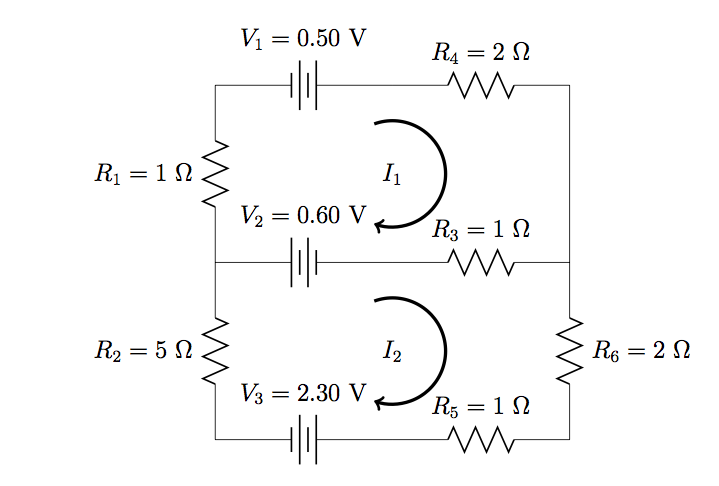
 ), and
 (there is a voltage drop across


![\[I_1=0.20~\mathrm{A},~~~I_2=-0.30~\mathrm{A}.\]](https://openpress.usask.ca/app/uploads/quicklatex/quicklatex.com-9964940c29fa03f8eacf4ac01f641745_l3.svg "Rendered by QuickLaTeX.com")
 to the right, the current in the top branch must be
  to the right, and the current in the centre branch must be
  to the left.
 for the potential difference with respect to the
  , then substituting into our loop rule expressions, we skip right to applying the loop rule for each mesh current and solve the system of fewer equations with fewer unknown variables.
 , where
  are
are  -matrix. When
 is the
  is the matrix formed by replacing the
 ![\[I_1=\frac{\mathrm{det}(\mathbf{R}_1)}{\mathrm{det}(\mathbf{R})}=\frac{\left|\begin{array}{cc}-1.10~\mathrm{V}&1~\Omega\\2.90~\mathrm{V}&-9~\Omega\end{array}\right|}{\left|\begin{array}{cc}-4~\Omega&1~\Omega\\1~\Omega&-9~\Omega\end{array}\right|}=\frac{9.90~\mathrm{V}\cdot\Omega-2.90~\mathrm{V}\cdot\Omega}{36~\Omega^2-1~\Omega^2}=0.20~\mathrm{A},\]](https://openpress.usask.ca/app/uploads/quicklatex/quicklatex.com-48d8fb3aad522bceb6d92cde7618cd6e_l3.svg "Rendered by QuickLaTeX.com")
![\[I_2=\frac{\mathrm{det}(\mathbf{R}_2)}{\mathrm{det}(\mathbf{R})}=\frac{\left|\begin{array}{cc}-4~\Omega&-1.10~\mathrm{V}\\1~\Omega&2.90~\mathrm{V}\end{array}\right|}{\left|\begin{array}{cc}-4~\Omega&1~\Omega\\1~\Omega&-9~\Omega\end{array}\right|}=\frac{-11.6~\mathrm{V}\cdot\Omega+1.10~\mathrm{V}\cdot\Omega}{35~\Omega^2-1~\Omega^2}=-0.30~\mathrm{A}.\]](https://openpress.usask.ca/app/uploads/quicklatex/quicklatex.com-4803d966ba6d91bf7b29361aa64d8fd0_l3.svg "Rendered by QuickLaTeX.com")
 , where
  was the mesh current in the loop of interest and
  was the adjacent mesh current. Indeed, in general when all the mesh current loops of a circuit are defined as pointing in the same direction—i.e. either clockwise or counterclockwise—the potential differences across all resistors
  located between adjacent mesh current loops are
  , where
  the potential difference across every voltage source and resistor will be:
 when
when  when only
  , and
, and
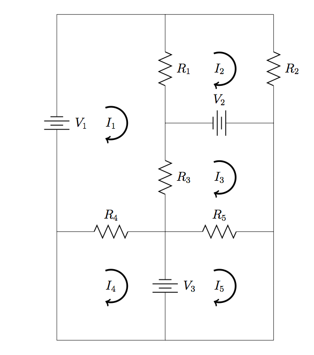

![\[\begin{array}{rccccc}V_1=&-(R_1+R_3+R_4)I_1&+R_1I_2&+R_3I_3&+R_4I_4&+0,\\V_2=&R_1I_1&-(R_1+R_2)I_2&+0&+0&+0,\\-V_2=&R_3I_1&+0&-(R_3+R_5)I_3&+0&+R_5I_5,\\-V_3=&R_4I_1&+0&+0&-R_4I_4&+0,\\V_3=&0&+0&+R_5I_3&+0&-R_5I_5.\end{array}\]](https://openpress.usask.ca/app/uploads/quicklatex/quicklatex.com-ade02c9effcc118a2d96258816b33cbb_l3.svg "Rendered by QuickLaTeX.com")
![\[\mathbf{V}=\left(\begin{array}{c}V_1\\V_2\\-V_2\\-V_3\\V_3\end{array}\right)\]](https://openpress.usask.ca/app/uploads/quicklatex/quicklatex.com-153885c8b26fdeaf4e4b238aa10171b1_l3.svg "Rendered by QuickLaTeX.com")
![\[\mathbf{R}=\left(\begin{array}{ccccc}-(R_1+R_3+R_4)&R_1&R_3&R_4&0\\R_1&-(R_1+R_2)&0&0&0\\R_3&0&-(R_3+R_5)&0&R_5\\R_4&0&0&-R_4&0\\0&0&R_5&0&-R_5\end{array}\right)\]](https://openpress.usask.ca/app/uploads/quicklatex/quicklatex.com-78a66446908a45f64b15bfc8908179a4_l3.svg "Rendered by QuickLaTeX.com")
 is negative the sum of voltage rises and drops due to voltage sources around each mesh current loop
  is negative the sum of the resistances of the resistors around mesh current loop
  is the sum of resistances of the resistors through which any mesh current loop
  . Similarly, the equation for loop
  for each voltage source
 that
that  for each voltage source
 that
that  for each resistor
 that
that 
 is the sum
  for each resistor
 passed by a loop
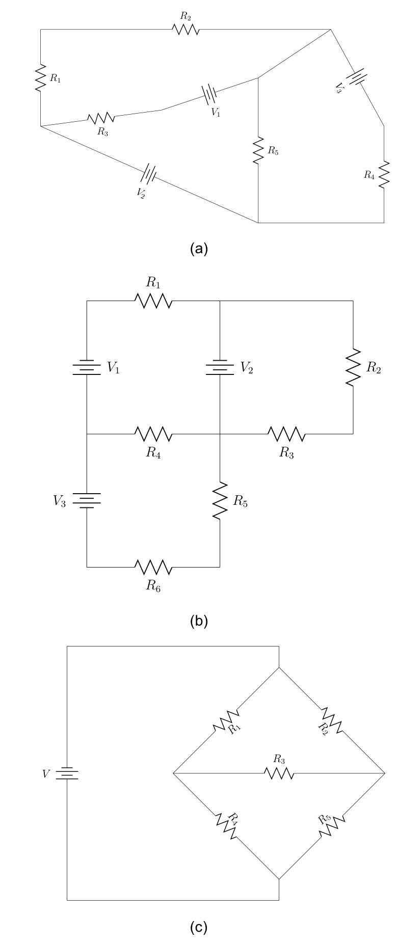

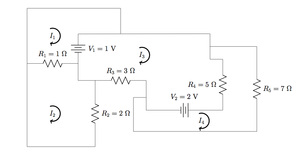

![\[\mathbf{V}=\left(\begin{array}{c}V_1\\0\\-V_1+V_2\\-V_2\end{array}\right)=\left(\begin{array}{c}1\\0\\1\\-2\end{array}\right)\]](https://openpress.usask.ca/app/uploads/quicklatex/quicklatex.com-62db9f63024cd32fbb40b037c213979e_l3.svg "Rendered by QuickLaTeX.com")


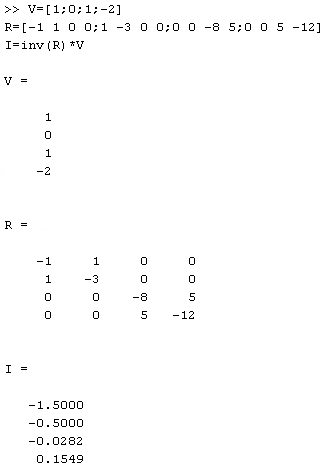
 to the right,
 upward,
 to the right,
 upward,
 downward,
 upward.
![\[P_{\mathrm{supplied}}=\sum_iI_{V_i}V_i=1.4718~\mathrm{W}+0.3662~\mathrm{W}=1.8380~\mathrm{W},\]](https://openpress.usask.ca/app/uploads/quicklatex/quicklatex.com-35b8036ebab70c4bad376dabd7999efa_l3.svg "Rendered by QuickLaTeX.com")


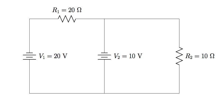
 Thus,
Thus,![\[I_{R_1}(V_1)=\frac{V_1}{R_1}=1~\mathrm{A}~\mathrm{to~left},~~~~~I_{R_2}(V_1)=\frac{0}{R_2}=0.\]](https://openpress.usask.ca/app/uploads/quicklatex/quicklatex.com-511f4fb3e1b270509237be2c826a7d9e_l3.svg "Rendered by QuickLaTeX.com")
![\[I_{R_1}(V_2)=\frac{V_2}{R_1}=0.5~\mathrm{A}~\mathrm{to~right},~~~~~I_{R_2}(V_2)=\frac{V_2}{R_2}=1~\mathrm{A}~\mathrm{upward}.\]](https://openpress.usask.ca/app/uploads/quicklatex/quicklatex.com-e5d75353af661681a48637b50bdf20ad_l3.svg "Rendered by QuickLaTeX.com")
![\[I_{R_1}=0.5~\mathrm{A}~\mathrm{to~left},~~~~~I_{R_2}=1~\mathrm{A}~\mathrm{upward}.\]](https://openpress.usask.ca/app/uploads/quicklatex/quicklatex.com-85dcd7ebb181d898e5ea241b0b2008f8_l3.svg "Rendered by QuickLaTeX.com")
 and points downwards, since
![\[P_{\mathrm{supplied}}=\sum_iI_{V_i}V_i=(0.5~\mathrm{A})(20~\mathrm{V})+(0.5~\mathrm{A})(10~\mathrm{V})=10~\mathrm{W}+5~\mathrm{W}=15~\mathrm{W}.\]](https://openpress.usask.ca/app/uploads/quicklatex/quicklatex.com-ae52e298d504eacd21fc5d1b356b9b2a_l3.svg "Rendered by QuickLaTeX.com")
![\[P_{\mathrm{dissipated}}=\sum_iI_{R_i}^2R_i=(0.5~\mathrm{A})^2(20~\Omega)+(1~\mathrm{A})^2(10~\Omega)=5~\mathrm{W}+10~\mathrm{W}=15~\mathrm{W}.\]](https://openpress.usask.ca/app/uploads/quicklatex/quicklatex.com-fef94adfd16f490a22740920f7f3f11c_l3.svg "Rendered by QuickLaTeX.com")
 source were replaced by a short? What if its voltage were doubled to
  ? Explain.
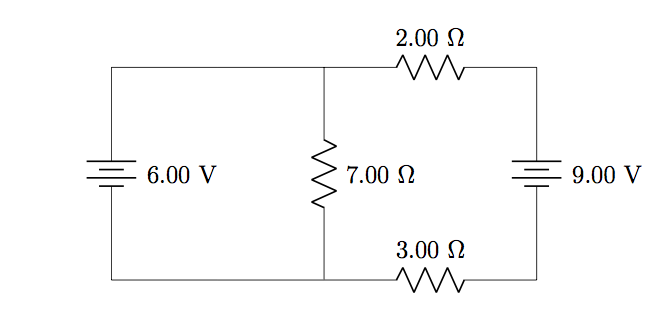

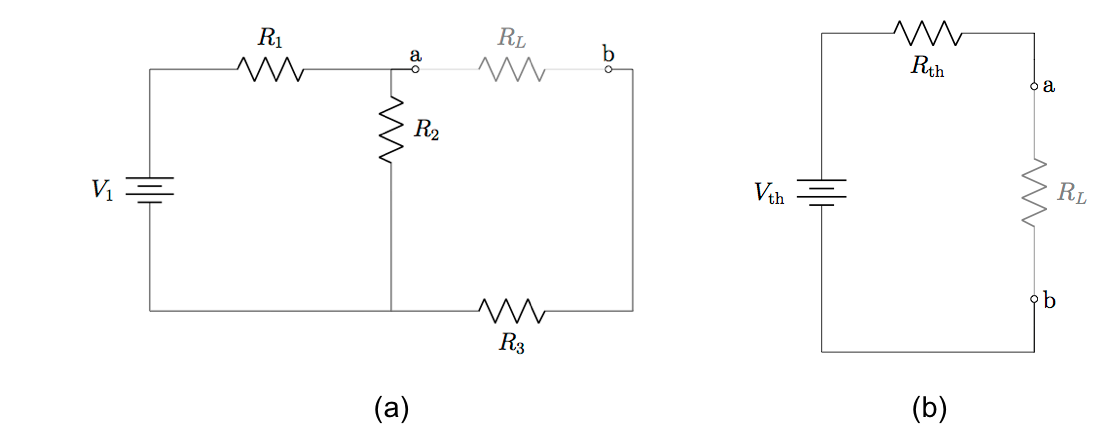


 .
.![\[I=\frac{V_1}{R_1+R_2}.\]](https://openpress.usask.ca/app/uploads/quicklatex/quicklatex.com-b4474e9fabae01d6328552d0691e2706_l3.svg "Rendered by QuickLaTeX.com")
![\[V_{R_2}=R_2I=\frac{R_2V_1}{R_1+R_2}.\]](https://openpress.usask.ca/app/uploads/quicklatex/quicklatex.com-4b23737c06725e9406391e94dd619c11_l3.svg "Rendered by QuickLaTeX.com")
![\[V_{\mathrm{th}}=V_{R_2}=\frac{R_2V_1}{R_1+R_2}.\]](https://openpress.usask.ca/app/uploads/quicklatex/quicklatex.com-44ad69d22a14ab539dac6ddcb91e5d59_l3.svg "Rendered by QuickLaTeX.com")
 first write
![\[R_{12}=\left(\frac{1}{R_1}+\frac{1}{R_2}\right)^{-1}=\frac{R_1R_2}{R_1+R_2}.\]](https://openpress.usask.ca/app/uploads/quicklatex/quicklatex.com-299b01eb56b9c53bf1097214b1d3af50_l3.svg "Rendered by QuickLaTeX.com")
![\[R_{\mathrm{th}}=R_{12}+R_3=\frac{R_1R_2}{R_1+R_2}+R_3.\]](https://openpress.usask.ca/app/uploads/quicklatex/quicklatex.com-5d1fac446c5ea68f8badfbf3b5111d3a_l3.svg "Rendered by QuickLaTeX.com")
![\[-(V_1-R_1I)=-V_1+\frac{R_1V_1}{R_1+R_2}=\frac{R_2V_1}{R_1+R_2}=R_{\mathrm{th}},\]](https://openpress.usask.ca/app/uploads/quicklatex/quicklatex.com-8846022e45862af5d70c249626aeb5fb_l3.svg "Rendered by QuickLaTeX.com")
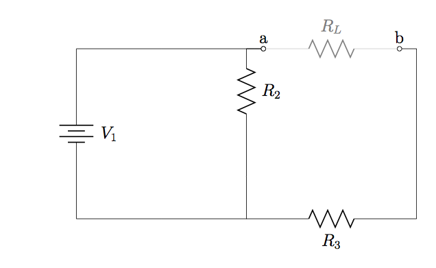
![\[\frac{dP_L}{dR_L}=\frac{V_{\mathrm{th}}^2}{(R_{\mathrm{th}}+R_L)^2}-\frac{2R_LV_{\mathrm{th}}^2}{(R_{\mathrm{th}}+R_L)^3}=0\]](https://openpress.usask.ca/app/uploads/quicklatex/quicklatex.com-3ebddaaadf91ae1a91177836ac53a002_l3.svg "Rendered by QuickLaTeX.com")
![\[\Rightarrow 1-\frac{2R_L}{R_{\mathrm{th}}+R_L}=0\]](https://openpress.usask.ca/app/uploads/quicklatex/quicklatex.com-7a2ab6d0c26305310d89a68c3783e3e8_l3.svg "Rendered by QuickLaTeX.com")
![\[\Rightarrow R_L=R_{\mathrm{th}}.\]](https://openpress.usask.ca/app/uploads/quicklatex/quicklatex.com-e7166167758a811b5213b61c212b9f28_l3.svg "Rendered by QuickLaTeX.com")
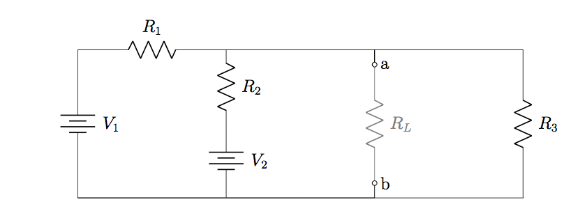
 for the Thévenin equivalent circuit calculated with respect to
  To find this, we first determine
  the other, passing through
  using Ohm’s law. Note that we do not actually need to calculate any other currents, since
  the potential difference between
  regardless which branch is taken.
 (see Equation
  (cf. Equation
 ![\[\left(\begin{array}{c}-V_1+V_2\\-V_2\end{array}\right)=\left(\begin{array}{cc}-(R_1+R_2)&R_2\\R_2&-(R_2+R_3)\end{array}\right)\left(\begin{array}{c}I_1\\I_2\end{array}\right),\]](https://openpress.usask.ca/app/uploads/quicklatex/quicklatex.com-f387a8e47d1e532c078948db5516ffb8_l3.svg "Rendered by QuickLaTeX.com")

![\[V_{\mathrm{th}}=R_3I_2=\frac{R_3(V_2R_1+V_1R_2)}{R_1R_2+R_1R_3+R_2R_3}.\]](https://openpress.usask.ca/app/uploads/quicklatex/quicklatex.com-265267cad54d2b27094933f31dd5b14c_l3.svg "Rendered by QuickLaTeX.com")
![\[R_{\mathrm{th}}=\left(\frac{1}{R_1}+\frac{1}{R_2}+\frac{1}{R_3}\right)^{-1}=\frac{R_1R_2+R_1R_3+R_2R_3}{R_1R_2R_3}.\]](https://openpress.usask.ca/app/uploads/quicklatex/quicklatex.com-463c326f46030c7e20be2c82b21f5735_l3.svg "Rendered by QuickLaTeX.com")
![\[P_{L,\mathrm{max}}=\frac{V_{\mathrm{th}}^2}{4R_{\mathrm{th}}}=\frac{R_1R_2R_3^3(V_2R_1+V_1R_2)^2}{(R_1R_2+R_1R_3+R_2R_3)^3}.\]](https://openpress.usask.ca/app/uploads/quicklatex/quicklatex.com-1fad99e2ff47b6d39d5850e569528091_l3.svg "Rendered by QuickLaTeX.com")
 is the power dissipated in
  The general expression for power dissipated in
 ![\[I_i=\frac{\mathrm{det}(\mathbf{R}_i)}{\mathrm{det}(\mathbf{R})},\]](https://openpress.usask.ca/app/uploads/quicklatex/quicklatex.com-a8ddcf648d0df8c46cfa89e358f47eb4_l3.svg "Rendered by QuickLaTeX.com")


 as the cross product of the velocity and magnetic field, that is,
 —in terms of the force on a charged particle moving in a magnetic field. The magnitude of the force is determined from the definition of the cross product as it relates to the magnitudes of each of the vectors. In other words, the magnitude of the force satisfies

 ), where
  , is sometimes used. The strongest permanent magnets have fields near
  ; superconducting electromagnets may attain
  or more. Earth’s magnetic field on its surface is only about
  or
or  .
.
 moves through a uniform magnetic field whose magnitude is
  . The field is directly parallel to the positive
  (b) in the negative
  ?
?
 or
or  to calculate the force. The direction of the force is determined by RHR-1.

 degrees. Therefore, the magnitude of the force is:
 or
or  direction possible, but not in the
  direction. This should match the mathematical answer. To calculate the force, we use the given charge, velocity, and magnetic field and the definition of the magnetic force in cross-product form to calculate:
 plane:


 s—like the tails of arrows). The magnetic force is perpendicular to the velocity, so velocity changes in direction but not magnitude. The result is uniform circular motion. (Note that because the charge is negative, the force is opposite in direction to the prediction of the right-hand rule.)
 . Noting that the velocity is perpendicular to the magnetic field, the magnitude of the magnetic force is reduced to
  . Because the magnetic force
  , we have


 of the helix, which is the distance between adjacent turns. This distance equals the parallel component of the velocity times the period:


 bends through a
  degree region with a uniform magnetic field of
  (
(

![\[T=\frac{2\pi m}{qB}=\frac{2\pi\left(6.64\times10^{-27}~\mathrm{kg}\right)}{\left(3.2\times10^{-19}~\mathrm{C}\right)(0.050~\mathrm{T})}=2.6\times10^{-6}~\mathrm{s}.\]](https://openpress.usask.ca/app/uploads/quicklatex/quicklatex.com-07379ec3030e1e22c514c3f35d6108ec_l3.svg "Rendered by QuickLaTeX.com")
![\[t=0.25\times2.61\times10^{-6}~\mathrm{s}=6.5\times10^{-7}~\mathrm{s}.\]](https://openpress.usask.ca/app/uploads/quicklatex/quicklatex.com-00fce32be7987150ffe2358aee1ba93b_l3.svg "Rendered by QuickLaTeX.com")
 ? (b) Compare this force with the weight
  of a proton.
 with a speed of
  . At what angle must the magnetic field be from the velocity so that the pitch of the resulting helical motion is equal to the radius of the helix?

 . The wire is formed from material that contains
  . If the charge carriers move with drift velocity
 ![\[I=neAv_d.\]](https://openpress.usask.ca/app/uploads/quicklatex/quicklatex.com-d8c0f8973c200f3be1c4b6c87f4559d7_l3.svg "Rendered by QuickLaTeX.com")
 , so the total magnetic force


 is suspended in a horizontal plane by a pair of flexible leads (
 , which is directed as shown. What are the magnitude and direction of the current in the wire needed to remove the tension in the supporting leads?
![\[mg=IlB.\]](https://openpress.usask.ca/app/uploads/quicklatex/quicklatex.com-22063141932d6601460ac06e31010577_l3.svg "Rendered by QuickLaTeX.com")
![\[I=\frac{mg}{lB}=\frac{(0.010~\mathrm{kg})(9.8~\mathrm{m/s}^2)}{(0.50~\mathrm{m})(0.50~\mathrm{T})}=0.39~\mathrm{A}.\]](https://openpress.usask.ca/app/uploads/quicklatex/quicklatex.com-e3c06843c6b4494c16eed02ed46b2d35_l3.svg "Rendered by QuickLaTeX.com")
 current flowing in the positive
  is directed along the positive
  axis towards the
  axis, what is the magnetic force per unit length on the wire?
 . For part a, since the current and magnetic field are perpendicular in this problem, we can simplify the formula to give us the magnitude and find the direction through the RHR-1. The angle
  . Also, the length can be divided over to the left-hand side to find the force per unit length. For part b, the current times length is written in unit vector notation, as well as the magnetic field. After the cross product is taken, the directionality is evident by the resulting unit vector.
![\[frac{\vec{\mathbf{F}}}{l}&=&1.5\hat{\mathbf{k}}~\mathrm{N/m}.\]](https://openpress.usask.ca/app/uploads/quicklatex/quicklatex.com-e2da00e9c90a1abfa31c9fdb22fb57af_l3.svg "Rendered by QuickLaTeX.com")

 direction?
![\[dF=IB\sin\theta dl.\]](https://openpress.usask.ca/app/uploads/quicklatex/quicklatex.com-4080c64c4d434a7e477c3678cf1a39ce_l3.svg "Rendered by QuickLaTeX.com")

 . This results in:
![\[F=IBR\int_0^{\pi}\sin\theta d\theta=IBR(-\cos\pi+\cos0)=2IBR.\]](https://openpress.usask.ca/app/uploads/quicklatex/quicklatex.com-727d7bdc9cd9727944ccf0b458884c0d_l3.svg "Rendered by QuickLaTeX.com")
![\[F=IBR\int_{\pi}^{0}\sin\theta d\theta=IBR(-\cos0+\cos\pi)=-2IBR.\]](https://openpress.usask.ca/app/uploads/quicklatex/quicklatex.com-2b2ef1ffc4c2f3f52159472e9e3908a1_l3.svg "Rendered by QuickLaTeX.com")

 . The magnetic force on a straight current-carrying wire of length
  . To find the net force on the loop, we have to apply this equation to each of the four sides. The force on side


 has been obtained for a rectangular loop, it is far more general and holds for current-carrying loops of arbitrary shapes; that is, there is no net force on a current loop in a uniform magnetic field.
 and
and  . Since they have the same line of action and are equal and opposite, the sum of their torques about any axis is zero (see
  and
and  . Let’s calculate the torques around the axis that passes through point
  from side
  and
and  , respectively, so the net torque on the loop is

 is the area of the loop.
 is known as its
  . Actually, the magnetic dipole moment is a vector that is defined as


 . (a) What is the magnitude of its magnetic dipole moment? (b) If the dipole is oriented at
  .
.![\[\mu=IA=(2.0\times10^{-3}~\mathrm{A})(\pi(0.02~\mathrm{m})^2)=2.5\times10^{-6}~\mathrm{A}\cdot\mathrm{m}^2\]](https://openpress.usask.ca/app/uploads/quicklatex/quicklatex.com-5ce0e02d79ec9fbe193369e51c6d458c_l3.svg "Rendered by QuickLaTeX.com")


 and
and  respectively. (a) What must the velocity of the electron beam be to traverse the crossed fields undeflected? If the electric field is turned off, (b) what is the acceleration of the electron beam and (c) what is the radius of the circular motion that results?
![\[v_{\mathrm{d}}=\frac{E}{B}=\frac{6\times10^3~\mathrm{N/C}}{2\times10^{-3}~\mathrm{T}}=3\times10^6~\mathrm{m/s}.\]](https://openpress.usask.ca/app/uploads/quicklatex/quicklatex.com-4247acbc1c1e16603570f57a2b633a74_l3.svg "Rendered by QuickLaTeX.com")

![\[r=\frac{mv}{qB}=\frac{(9.1\times10^{-31}~\mathrm{kg})(3\times10^{6}~\mathrm{m/s})}{(1.6\times10^{-19}~\mathrm{C})(2\times10^{-3}~\mathrm{T})}=8.5\times10^{-3}~\mathrm{m}.\]](https://openpress.usask.ca/app/uploads/quicklatex/quicklatex.com-ee68c37d2ab01a09e1b1752993118082_l3.svg "Rendered by QuickLaTeX.com")
 . The ribbon carries a current of
  from left to right, and it lies in a uniform magnetic field of magnitude
  electrons per cubic meter for silver, find the Hall potential between the edges of the ribbon.
![\[V=\frac{IBl}{neA}.\]](https://openpress.usask.ca/app/uploads/quicklatex/quicklatex.com-5528b0a212b3a6e8e3c2f442b7441e2c_l3.svg "Rendered by QuickLaTeX.com")

 electrons per cubic meter, which is
  thick. What is the magnetic field when
  and the Hall potential is (a)
  and (b)
 since any ion with a different velocity is deflected preferentially by either the electric or magnetic force, and ultimately blocked from the next stage. They then enter a uniform magnetic field
  where they travel in a circular path whose radius
 and the radius
 , measured values of
  .
. . The performance of the refrigerator is severely hampered if even a minute leak between its various components occurs. Consequently, before it is cooled down to the desired temperature, the refrigerator is subjected to a leak test. A small quantity of gaseous helium is injected into one of its compartments, while an adjacent, but supposedly isolated, compartment is connected to a high-vacuum pump to which a mass spectrometer is attached. A heated filament ionizes any helium atoms evacuated by the pump. The detection of these ions by the spectrometer then indicates a leak between the two compartments of the dilution refrigerator.
 and
and  , called
 , where

 , the polarity of the dees is reversed. When the particle reenters the gap,

 . Above this energy, relativistic effects become important, which causes the orbital period to increase with the radius. Up to energies of several hundred
  long and accelerates electrons and positrons (positively charged electrons) to energies of
  . The synchrotron is constructed so that its bending magnetic field increases with particle speed in such a way that the particles stay in an orbit of fixed radius. The world’s highest-energy synchrotron is located at CERN, which is on the Swiss-French border near Geneva. CERN has been of recent interest with the verified discovery of the Higgs Boson. This synchrotron can accelerate beams of approximately
  protons to energies of about
  .
. ,
,  has a radius of
  and a magnetic field of
  . (a) What is the period of revolution of the alpha-particles? (b) What is their maximum kinetic energy?
![\[T=\frac{2\pi m}{qB}=\frac{2\pi\left(6.64\times10^{-27}~\mathrm{kg}\right)}{\left(3.2\times10^{-19}~\mathrm{C}\right)(1.8~\mathrm{T})}=7.3\times10^{-8}~\mathrm{s}.\]](https://openpress.usask.ca/app/uploads/quicklatex/quicklatex.com-5ca85193aa1b8d6610367e0648ce3779_l3.svg "Rendered by QuickLaTeX.com")

 using a magnetic field of
  . What is the required radius of the cyclotron?
 unit of the magnetic field strength;


 The force is perpendicular to the plane formed by


 on a current-carrying loop of any shape in a uniform magnetic field is calculated using
  is the magnetic dipole moment and
  the current in the loop
  or
or 

 b.
b.  c.
c.  d.
d. 
 toward the south; b.
 b.
b. 


 over Earth’s south magnetic pole, where the
  magnetic field points straight up. What are the direction and the magnitude of the magnetic force on the plane? (b) Discuss whether the value obtained in part (a) implies this is a significant or negligible effect.
 experiences a magnetic force of
  What is the strength of the magnetic field if there is a
  in a
in a  magnetic field experiences a magnetic force of
  What angle does the velocity of the electron make with the magnetic field? There are two answers.
 What is the greatest the charge can be if it moves at a maximum speed of
  in Earth’s field? (b) Discuss whether it would be difficult to limit the charge to less than the value found in (a) by comparing it with typical static electricity and noting that static is often absent.
 perpendicular to Earth’s magnetic field at an altitude where the field strength is
  What is the radius of the circular path the electron follows?
 in a circular path
  in radius? Antiprotons have the same mass as protons but the opposite (negative) charge. (b) Is this field strength obtainable with today’s technology or is it a futuristic possibility?
 travels at
  perpendicular to a
  magnetic field, which makes it move in a circular arc with a
  radius. What positive charge is on the ion? (b) What is the ratio of this charge to the charge of an electron? (c) Discuss why the ratio found in (b) should be an integer.
 in a direction perpendicular to Earth’s field, which has a strength of
  (a) What strength electric field must be applied perpendicular to the Earth’s field to make the electron moves in a straight line? (b) If this is done between plates separated by
  what is the voltage applied? (Note that TVs are usually surrounded by a ferromagnetic material to shield against external magnetic fields and avoid the need for such a correction.)
 ? (b) Find the radius of curvature of the path of a proton accelerated through this potential in a
  field and compare this with the radius of curvature of an electron accelerated through the same potential.
 travels in a circular path of radius
  (a) What is the speed of the particle? (b) What is the kinetic energy in electron-volts? (c) Through what potential difference must the particle be accelerated in order to give it this kinetic energy?
 what is the radius of its circular orbit?
 perpendicular to Earth’s
  ? (b) What is the direction of the force if the current is straight up and Earth’s field direction is due north, parallel to the ground?
 at an angle of
  to Earth’s
  field. What is the force on a
  section of this line? (b) Discuss practical concerns this presents, if any.
 current passes between the poles of a strong magnet that is perpendicular to its field and experiences a
  force on the
  of their strength? (b) How many percent would the current need to be increased to return the torque to original values?
 on a side that carries a
  current in a
  field? (b) What is the torque when
  ?
? The loop has
  square turns that are
  on a side and is in a uniform
  magnetic field.
 -turn square loop
  if the loop is carrying
 must equal units of
  Verify this.
 of maximum? (c)
  of maximum?
 in radius with a current of
  Find the maximum torque on a proton in a
  field. (This is a significant torque on a small particle.)
 is vertical, with its axis on an east-west line. A current of
  What are the direction and magnitude of the torque on the loop? (b) Does this device have any practical applications as a motor?
 below the horizontal and with a strength of
 The Hall electric field is measured to be
  (a) What is the drift speed of the conduction electrons? (b) Assuming that
  electrons per cubic meter and that the cross-sectional area of the strip is
  calculate the current in the strip. (c) What is the Hall coefficient
  ?
? and it is placed in a magnetic field of magnitude
  What are the value and polarity of the Hall potential in the copper strip?
 and
and  respectively. (a) What speed must a proton have to pass through the selector? (b) Also calculate the speeds required for an alpha-particle and a singly ionized
  atom to pass through the selector.
 and
and  When the electric field is turned off, the charged particle travels in a circular path of radius
  Determine the charge-to-mass ratio of the particle.
 for a current of
  when it is placed in a magnetic field of
  What is the magnetic field in a region where the reading is
  for
for  of current?
 Determine (a) the rotational period of the circulating protons and (b) the maximum radius of the protons’ orbit.
 and
and  and the strength of the magnetic field that separates the ions is
  A stream of singly charged
  ions is found to bend in a circular arc of radius
  What is the mass of the
  and the maximum orbital radius of the circulating protons is
  (a) What is the kinetic energy of the protons when they are ejected from the cyclotron? (b) What is this energy in
  taken from a sample of old glacial ice. (The relative abundance of these oxygen isotopes is related to climatic temperature at the time the ice was deposited.) The ratio of the masses of these two ions is
  and they are singly charged and travel at
  and uranium-
 ions are being separated in a mass spectrometer. (The much rarer uranium-
 and
and  respectively, and they travel at
  in a
in a  field. What is the separation between their paths when they hit a target after traversing a semicircle? (b) Discuss whether this distance between their paths seems to be big enough to be practical in the separation of uranium-
 moving with a velocity of
  in a magnetic field of

 with a velocity of
  What is the magnetic force on the electron?
 and
and  respectively. If the droplet is given an initial horizontal velocity of
  what magnetic field will keep it moving in this direction? Why must gravity be considered here?
 and
and 
 passes between parallel plates that are
  What is the strength of the uniform magnetic field
  enters a region where
  and
and  What is the initial force on it?
 enters a region where there is a uniform electric field and a uniform magnetic field. The magnetic field is given by
  If the electron travels through a region without being deflected, what is the electric field?
 Earth’s magnetic field has a horizontal component of
  north and a vertical component of
  to a circular orbit of radius
  to complete eight revolutions in a uniform magnetic field of magnitude
 enters a uniform magnetic field that is horizontal and directed from east to west. (a) If the particle is deflected initially to the north in a circular arc, is its charge positive or negative? (b) If
  and the charge-to-mass ratio
  of the particle is
  what is the radius of the path? (c) What is the speed of the particle after it has moved in the field for
  ? for
? for  ?
? and
and 
 completes
  Identify the ion.
 of the radii of their circular orbits?
 and travels in a helical path with a radius of
  (a) What is the value of
  after entering the field?
 angle with the
  Calculate the (a) pitch and (b) radius of the trajectory.
 -long section of cable carrying current to a car starter motor makes an angle of
  field. What is the current when the wire experiences a force of
  ? (b) If you run the wire between the poles of a strong horseshoe magnet, subjecting
  what force is exerted on this segment of wire?
 current and the
  ? (b) What is the force on the wire if it is rotated to make an angle of
  -long segment of wire lies along the
  in the positive
  Find the magnetic force on this segment.
 section of a long, straight wire carries a current of
  Calculate the magnitude of the force on the section if the angle between the field and the direction of the current is (a)
  (b)
(b)  (c)
(c)  or (d)
  passes through the field as shown in the accompanying figure. What is the magnetic force on the wire?
 and
and  If the coil is placed in a uniform magnetic field of strength
  what is the maximum torque on it?
 The coil lies in a magnetic field of magnitude
  of the maximum possible torque. What is the angle between the magnetic field and the normal to the plane of the coil?
 by
by  rectangular current loop carries a current of
  What is the magnetic dipole moment of the loop?
 (a) What current through the coil results in a magnetic dipole moment of
  ? (b) What is the maximum torque that the coil will experience in a uniform field of strength
  ? (c) If the angle between
  what is the magnitude of the torque on the coil? (d) What is the magnetic potential energy of coil for this orientation?
 magnetic field such that
  and it is placed in a uniform magnetic field of strength
  (a) What is the maximum torque that the loop will experience if it is square? (b) If it is circular? (c) At what angle relative to
  Show that the magnitudes of the magnetic dipole moment
 ![\[\frac{\mu}{L}=\frac{e}{2m}.\]](https://openpress.usask.ca/app/uploads/quicklatex/quicklatex.com-edf87790ecc475f6bb63925a8bd83c8f_l3.svg "Rendered by QuickLaTeX.com")
 electrons per cubic meter. What will be the Hall voltage reading from a probe made up of
  copper plate when a current of
  is passed through it in a magnetic field of
  perpendicular to the
 for
for  current is observed in a
  magnetic field for a rectangular sample with length
  width
width  and height
  Determine the density of the charge carriers.
 magnetic field. (a) What electric field strength is needed to select a speed of
  proton moving perpendicularly to the
  field of a cyclotron.
 -diameter pipe if the Hall voltage is
  (b) What would the Hall voltage be for the same flow rate through a
  -diameter pipe with the same field applied?
 (that of a helium atom) moving at
  perpendicular to a
  magnetic field travels in a circular path of radius
  (a) What is the charge of the particle? (b) What is unreasonable about this result? (c) Which assumptions are responsible?
 -long wire perpendicular to Earth’s
  field. (a) Find the speed with which the wire must move. (b) What is unreasonable about this result? (c) Which assumption is responsible?
 output for blood moving at
  in a
in a  -diameter vessel. (a) What magnetic field strength is needed? (b) What is unreasonable about this result? (c) Which premise is responsible?
 pointed in the
  -direction as it crosses the
  at a particular time. There is a negative charge
  pointed in the
  -direction. It is found that the particle describes a circle of radius
  Find
Find  enters a region of uniform magnetic field of
  at an angle of
  to the magnetic field. In the region of magnetic field proton describes a helical path with radius
 entering a region of uniform magnetic field
  over a
 and
and  where
where  a wire of length
  Find the magnetic force on the wire at this instant in time.
 A uniform magnetic field of magnitude
  a chamber in which a gas discharge is taking place. The ion is accelerated by a potential difference
  and allowed to enter a region of constant magnetic field
  In the uniform magnetic field region, the ion moves in a semicircular path striking a photographic plate at a distance

 and
and 

 and the ring rotates about the
  in the positive
  with
with  and
and 
 carries a current of
  At a particular instant, the loop lies in the
  As viewed from above the
 due to an element

 produces a magnetic field at point P given by the Biot-Savart law.
 is known as the
 . The magnitude of
 , then
  \vec{\mathbf{0}}

 . Another way to think about it is that each of the radius values is nearly the same, no matter where the current element is on the line segment, if
  and
and ![\[\theta=\tan^{-1}\left(\frac{1~\mathrm{m}}{0.01~\mathrm{m}}=89.4^{\circ}.\right)\]](https://openpress.usask.ca/app/uploads/quicklatex/quicklatex.com-c2dbd9ba4167b8a6adeabc9d098910ef_l3.svg "Rendered by QuickLaTeX.com")


![\[B=\frac{\mu_0}{4\pi}\int_{\mathrm{wire}}\frac{Id\vec{\mathbf{l}}\times\hat{\mathbf{r}}}{r^2}.\]](https://openpress.usask.ca/app/uploads/quicklatex/quicklatex.com-93380b0bee5cc0004a48cb6eb7620ec4_l3.svg "Rendered by QuickLaTeX.com")
 :
:![\[B=\frac{\mu_0}{4\pi}\int_{\mathrm{wire}}\frac{Ird\theta}{r^2}.\]](https://openpress.usask.ca/app/uploads/quicklatex/quicklatex.com-3f384a3127976d3cc3add8a731f7153a_l3.svg "Rendered by QuickLaTeX.com")
![\[B=\frac{\mu_0I}{4\pi r}\int_{\mathrm{wire}}d\theta.\]](https://openpress.usask.ca/app/uploads/quicklatex/quicklatex.com-90f76ff05922d11016e59efada82510a_l3.svg "Rendered by QuickLaTeX.com")
![\[B=\frac{\mu_0I\theta}{4\pi r}.\]](https://openpress.usask.ca/app/uploads/quicklatex/quicklatex.com-cb4632e378f8939a2cbe19fb0180a029_l3.svg "Rendered by QuickLaTeX.com")

 and
and  .
. located at the position
  points out of the page for any element along the wire. At point
  , we have from the Biot-Savart law
 in terms of
 ![\[r=\sqrt{x^2+R^2}\]](https://openpress.usask.ca/app/uploads/quicklatex/quicklatex.com-9d070377a57bc8256787cdf817ed6a1f_l3.svg "Rendered by QuickLaTeX.com")
![\[\sin\theta=\frac{R}{\sqrt{x^2+R^2}}.\]](https://openpress.usask.ca/app/uploads/quicklatex/quicklatex.com-63c539c3b49166c81d44003f45abf31c_l3.svg "Rendered by QuickLaTeX.com")

![\begin{equation*}B=\frac{\mu_0I}{2\pi R}\left[\frac{x}{(x^2+R^2)^{1/2}}\right]_0^{\infty}.\end{equation*}](https://openpress.usask.ca/app/uploads/quicklatex/quicklatex.com-cd8df5fbf8e0fbfa17418669324a5702_l3.svg "Rendered by QuickLaTeX.com")


![\[B_1=B_3=\frac{\mu_0I}{2\pi R}=\frac{(4\pi\times10^{-7}~\mathrm{T}\cdot\mathrm{m/A})(2~\mathrm{A})}{2\pi(0.01~\mathrm{m})}=4\times10^{-5}~\mathrm{T}.\]](https://openpress.usask.ca/app/uploads/quicklatex/quicklatex.com-7fa361e942d60f5e3360eab0ede4a2b7_l3.svg "Rendered by QuickLaTeX.com")
![\[B_2=\frac{\mu_0I}{2\pi R}=\frac{(4\pi\times10^{-7}~\mathrm{T}\cdot\mathrm{m/A})(2~\mathrm{A})}{2\pi(0.01414~\mathrm{m})}=3\times10^{-5}~\mathrm{T}.\]](https://openpress.usask.ca/app/uploads/quicklatex/quicklatex.com-bfe55c504aeff9862e58289b3a3ecb82_l3.svg "Rendered by QuickLaTeX.com")
![\[B_{\mathrm{net}~x}=-4\times10^{-5}~\mathrm{T}-(2.83\times10^{-5}~\mathrm{T})\cos(45^{\circ})=-6\times10^{-5}~\mathrm{T}.\]](https://openpress.usask.ca/app/uploads/quicklatex/quicklatex.com-47dc5e6ba94ab48a02bf6cee35fe9706_l3.svg "Rendered by QuickLaTeX.com")
![\[B_{\mathrm{net}~y}=-4\times10^{-5}~\mathrm{T}-(2.83\times10^{-5}~\mathrm{T})\sin(45^{\circ})=-6\times10^{-5}~\mathrm{T}.\]](https://openpress.usask.ca/app/uploads/quicklatex/quicklatex.com-2f921858e706793efbef4db927b1d05a_l3.svg "Rendered by QuickLaTeX.com")


 with
with 
 .) Since the wires are very long, it is convenient to think in terms of
  , the force per unit length. Substituting the expression for
  into Equation

 by definition, and because
  , the force per meter is exactly
  . This is the basis of the definition of the ampere.
 . For both the ampere and the coulomb, the method of measuring force between conductors is the most accurate in practice.
 . The first wire is located at
  while the other wire is located at
  as shown in
![\[r=\sqrt{(3.0~\mathrm{cm})^2+(4.0~\mathrm{cm})^2}=5.0~\mathrm{cm}.\]](https://openpress.usask.ca/app/uploads/quicklatex/quicklatex.com-96839640eb509bebaf695a8e1546fe65_l3.svg "Rendered by QuickLaTeX.com")
![\[\frac{F}{l}=\frac{\left(4\pi\times10^{-7}~\mathrm{T}\cdot\mathrm{m/A}\right)\left(5\times10^{-3}~\mathrm{A}\right)^2}{2\pi(5\times10^{-2}~\mathrm{m})}=1\times10^{-10}~\mathrm{N/m}.\]](https://openpress.usask.ca/app/uploads/quicklatex/quicklatex.com-7be2ac90f24fcfba799b9e52634636e7_l3.svg "Rendered by QuickLaTeX.com")
![\[\theta=\tan^{-1}\left(\frac{3~\mathrm{cm}}{4~\mathrm{cm}}\right)=36.9^{\circ}.\]](https://openpress.usask.ca/app/uploads/quicklatex/quicklatex.com-a7e69d862976f03db21ee7eab865cefd_l3.svg "Rendered by QuickLaTeX.com")
![\[\cos(36.9^{\circ})\hat{\mathbf{i}}-\sin(36.9^{\circ})\hat{\mathbf{j}}=0.8\hat{\mathbf{i}}-0.6\hat{\mathbf{j}}.\]](https://openpress.usask.ca/app/uploads/quicklatex/quicklatex.com-520cf16a5d1e4d57643ee52e6b78a0ae_l3.svg "Rendered by QuickLaTeX.com")
![\[\frac{\vec{\mathbf{F}}}{l}=(1\times10^{-10}~\mathrm{N/m})\times(0.8\hat{\mathbf{i}}-0.6\hat{\mathbf{j}})=(8\times10^{-11}\hat{\mathbf{i}}-6\times10^{-11}\hat{\mathbf{j}})~\mathrm{N/m}.\]](https://openpress.usask.ca/app/uploads/quicklatex/quicklatex.com-10d40e40217a98fdbdf178d9d497d48c_l3.svg "Rendered by QuickLaTeX.com")
![\[\frac{\vec{\mathbf{F}}}{l}=(-8\times10^{-11}\hat{\mathbf{i}}+6\times10^{-11}\hat{\mathbf{j}})~\mathrm{N/m}.\]](https://openpress.usask.ca/app/uploads/quicklatex/quicklatex.com-e5009625ac5da5e4b0ca062a099274ba_l3.svg "Rendered by QuickLaTeX.com")
 , respectively. The first wire is located at
  while the other wire is located at
  . What is the magnitude of the magnetic force per unit length of the first wire on the second and the second wire on the first?

 .
. due to the current element
  , which is directly opposite
![\[\cos\theta=\frac{R}{\sqrt{y^2+R^2}}.\]](https://openpress.usask.ca/app/uploads/quicklatex/quicklatex.com-49a6f21ab20805d81134cb5fbb47a1a2_l3.svg "Rendered by QuickLaTeX.com")

 . As discussed in the previous chapter, the closed current loop is a magnetic dipole of moment
  . For this example,
  and
and  , so the magnetic field at
 in Equation
 for a flat coil of n loops per length. It can also be expressed as
 in Equation

 , but flow in opposite directions as seen in
  while the other loop has a radius of
  . The distance from the first loop to the point where the magnetic field is measured is
  . What is the magnitude of the net magnetic field at point

 over the closed paths
  is the product of
  , and
, and![\[\vec{\mathbf{B}}\cdot d\vec{\mathbf{l}}=Brd\theta.\]](https://openpress.usask.ca/app/uploads/quicklatex/quicklatex.com-255a93c54eb608fe523aeefe810ee3cd_l3.svg "Rendered by QuickLaTeX.com")

 equals
  and
and 
 and
and
 (see
(see 


 and solve for
 and
and  , are shown at arbitrary points on a circle of radius
  . Therefore, we can apply Ampère’s law to the circular path as shown.
![\[\oint\vec{\mathbf{B}}\cdot d\vec{\mathbf{l}}=B_{\theta}\oint dl=B_{\theta(2\pi r).\]](https://openpress.usask.ca/app/uploads/quicklatex/quicklatex.com-d29109e897856ee622a4cc55335f17a5_l3.svg "Rendered by QuickLaTeX.com")
![\[B_{\theta}(2\pi r)=\mu_0I.\]](https://openpress.usask.ca/app/uploads/quicklatex/quicklatex.com-f0170010a9359f6cdabfa67e3a9f3251_l3.svg "Rendered by QuickLaTeX.com")
![\[B=\frac{\mu_0I}{2\pi r}.\]](https://openpress.usask.ca/app/uploads/quicklatex/quicklatex.com-762d302c98721fdf6e3c1ffb77fdb9a2_l3.svg "Rendered by QuickLaTeX.com")
 that is distributed uniformly over its cross-section. Find the magnetic field both inside and outside the wire.
![\[\oint\vec{\mathbf{B}}\cdot d\vec{\mathbf{l}}=\oint Bdl=B\oint dl=B(2\pi r).\]](https://openpress.usask.ca/app/uploads/quicklatex/quicklatex.com-690a30253b792a04aec7b678dc609883_l3.svg "Rendered by QuickLaTeX.com")
 such as that shown in part (a) of
  times the area enclosed. Since the current is uniform, the current density inside the path equals the current density in the whole wire, which is
  . Therefore the current
 ![\[I=\frac{\pi r^2}{\pi a^2}I_0=\frac{r^2}{a^2}I_0.\]](https://openpress.usask.ca/app/uploads/quicklatex/quicklatex.com-11e32ecb8e6fa9e54af77c91086ff5aa_l3.svg "Rendered by QuickLaTeX.com")
![\[B(2\pi r)=\mu_0\left(\frac{r^2}{a^2}\right)I_0,\]](https://openpress.usask.ca/app/uploads/quicklatex/quicklatex.com-52c8e7c84133018a45bb672afc88d49d_l3.svg "Rendered by QuickLaTeX.com")
![\[B=\frac{\mu_0I_0}{2\pi}\frac{r}{a^2}~(r\leq a).\]](https://openpress.usask.ca/app/uploads/quicklatex/quicklatex.com-0080742212d225a2551c8df65d9e7c38_l3.svg "Rendered by QuickLaTeX.com")
![\[B=\frac{\mu_0I_0}{2\pi r}~(r\geq a).\]](https://openpress.usask.ca/app/uploads/quicklatex/quicklatex.com-1085f9d29aacbf00e4974cf09effdc59_l3.svg "Rendered by QuickLaTeX.com")


 where
where  by finding the net current through the loop. Positive currents flow with your right-hand thumb if your fingers wrap around in the direction of the loop. This will tell us the sign of the answer.
 .
. .
. of current going downward and
  going upward. Therefore, the total current is
  and
and  .
. ; therefore, the number of turns in an infinitesimal length
  are
are  turns. This produces a current
 is the current through each slice. The magnetic field


![\begin{eqnarray*}\cos\theta d\theta&=&\left[-\frac{y^2}{(y^2+R^2)^{3/2}}+\frac{1}{\sqrt{y^2+R^2}}\right]dy\\&=&\frac{R^2dy}{(y^2+R^2)^{3/2}}.\end{eqnarray*}](https://openpress.usask.ca/app/uploads/quicklatex/quicklatex.com-4fbe3d0a263eac5880524c4e54b1f454_l3.svg "Rendered by QuickLaTeX.com")

 . From a practical point of view, the infinite solenoid is one whose length is much larger than its radius
  . In this case,
  and
and  . Then from Equation
 ![\[\vec{\mathbf{B}}=\frac{\mu_0IN}{2L}\hat{\mathbf{j}}[\sin(\pi/2)-\sin(-\pi/2)]=\frac{\mu_0IN}{L}\hat{\mathbf{j}}\]](https://openpress.usask.ca/app/uploads/quicklatex/quicklatex.com-34c6628910f7faa1c5f3ec5e83aca510_l3.svg "Rendered by QuickLaTeX.com")


 . Therefore, from Ampère’s law,
![\[Bl=\mu_0nlI\]](https://openpress.usask.ca/app/uploads/quicklatex/quicklatex.com-f8eb048ef2cad2ff5cb9e094781fb6a3_l3.svg "Rendered by QuickLaTeX.com")


 turns wound around a cylinder of diameter
  and length
  . If the current through the coils is
  , what is the magnitude of the magnetic field inside and near the middle of the solenoid?
![\[n=\frac{300~\mathrm{turns}}{0.140~\mathrm{m}}=2.14\times10^3~\mathrm{turns/m}.\]](https://openpress.usask.ca/app/uploads/quicklatex/quicklatex.com-fd7837075862ee45c1cdaf86b83c0dbb_l3.svg "Rendered by QuickLaTeX.com")

 ? (b)
? (b)  ? The solenoid has
  flowing through the coils
 . Actually, this assumption is not precisely correct, for as part (b) of
  ,
,  , and
, and  shown in part (d) of
![\[\oint B(2\pi r)=0\]](https://openpress.usask.ca/app/uploads/quicklatex/quicklatex.com-a4c0f5469f094c7793473fca51c30581_l3.svg "Rendered by QuickLaTeX.com")

 through the surface. We now find with Ampère’s law,
![\[B(2\pi r)=\mu_0NI\]](https://openpress.usask.ca/app/uploads/quicklatex/quicklatex.com-4c7e1d0c97a17d727e7cf6b5aefe10cd_l3.svg "Rendered by QuickLaTeX.com")

 .
.
 )
)

 atoms and ions, each with its magnetic dipole moment. If no external magnetic field is present, the magnetic dipoles are randomly oriented—as many are pointed up as down, as many are pointed east as west, and so on. Consequently, the net magnetic dipole moment of the sample is zero. However, if the sample is placed in a magnetic field, these dipoles tend to align with the field (see
  . If
. If  (the value of atomic hydrogen) and
  , then
![\[U_B=1.9\times10^{-23}~\mathrm{J}.\]](https://openpress.usask.ca/app/uploads/quicklatex/quicklatex.com-698e9dcd4905a24228af15e0edd07a62_l3.svg "Rendered by QuickLaTeX.com")
 ,
,![\[U_T\approx kT=(1.38\times10^{-23}~\mathrm{J/K})(300~\mathrm{K})=4.1\times10^{-21}~\mathrm{J},\]](https://openpress.usask.ca/app/uploads/quicklatex/quicklatex.com-321c4717d503e6f680051f1bdcf6ac4d_l3.svg "Rendered by QuickLaTeX.com")
 times greater than


 is the field due to the surface current
 is a dimensionless quantity called the

 . However, since


 )
)

 )
)


 to
to  , and they contain about
  to
to  atoms. Within a domain, the magnetic dipoles are rigidly aligned in the same direction by coupling among the atoms. This coupling, which is due to quantum mechanical effects, is so strong that even thermal agitation at room temperature cannot break it. The result is that each domain has a net dipole moment. Some materials have weaker coupling and are ferromagnetic only at lower temperatures.
 to
to  , and it also depends on the history of the magnetic field to which the material has been subject. A typical plot of
  ,
,  , and
, and  ; (2) for
  ,
,  , and
, and  .
.
 (i.e., when the current in the solenoid is turned off). The iron stays magnetized, which means that it has become a permanent magnet.


 turns per centimetre, what is the applied field
  ? (b) What is the net magnetic field for this same current? (c) What is the magnetic susceptibility in this case?
 . Notice that the internal field of the aligned atoms is much larger than the externally applied field.
![\[\chi=\frac{B}{B_0}-1=\frac{1.4~\mathrm{T}}{5.0\times10^{-4}~\mathrm{T}}-1=2.8\times10^3.\]](https://openpress.usask.ca/app/uploads/quicklatex/quicklatex.com-8887f48a392350fd4a88ec82e39deb17_l3.svg "Rendered by QuickLaTeX.com")
 .
. measure of the ability of a material, in this case free space, to support a magnetic field


 (at Center of loop)


 produces a magnetic field a distance
  is the permeability of free space.
![\[B=\mu_0nI\]](https://openpress.usask.ca/app/uploads/quicklatex/quicklatex.com-3c099d16e33bd664ab77eb91c279a8d4_l3.svg "Rendered by QuickLaTeX.com")
![\[B=\frac{\mu_0NI}{2\pi r}\]](https://openpress.usask.ca/app/uploads/quicklatex/quicklatex.com-fa334311233b7d0a929661a29fff96ec_l3.svg "Rendered by QuickLaTeX.com")


 b.
b. 
 b.
b.  c.
c. 
 inside a long, hollow copper pipe that is carrying an electric current parallel to the axis. Is
  current flows through the wire shown. What is the magnitude of the magnetic field due to a
  segment of wire as measured at (a) point A and (b) point B?
 segment that connects the longer wires as shown. Calculate the magnitude of the magnetic field at the center of the loop.
 are positioned as shown in the accompanying figure. If both wires carry a current
  Estimate the magnetic field
  What is the current through the long wire?
 above the ground carries a current of
  What is the magnetic field on the ground directly below the wire? Compare your answer with the magnetic field of Earth.
 If the wire is placed in a uniform magnetic field of magnitude
  that is directed vertically downward, what is the resultant magnitude of the magnetic field
  and
and  what is the magnetic field at point P?
 in the same direction, what is the magnetic force per meter exerted on each wire? (b) Does the force pull the wires together or push them apart? (c) What happens if the currents flow in opposite directions?
 the other a current of
  as shown in the accompanying figure. Each wire has a mass per unit length of
  and they carry the same current in opposite directions. What is the current if the cords hang at
  with respect to the vertical?
 The rectangular loop, whose long sides are parallel to the wire, carries a current
  What are the magnitude and direction of the force on the rectangular loop due to the magnetic field of the wire?
 the magnetic field at its center is
  What is the radius of the loop?
 ?
? At what distance along the axis of the loop is the magnetic field one-half its value at the center of the loop?
 for the paths
  and
and 
 Evaluate
  carries a current of
  What is the magnetic field just outside the wire?
 and outer radius
  A
A  current distributed uniformly over the cross-section flows into the page. Calculate the magnetic field at

 (b)
(b)  (c)
(c)  and (d)
  Assume that the current is distributed uniformly over the cross sections of the two parts of the cable.
 what is the magnetic field within the solenoid?
 within the solenoid?
 within it?
 long, has a diameter of
  and is wound with
  turns. If the current through the windings is
  what is the magnetic field at a point on the axis of the solenoid that is (a) at the center of the solenoid, (b)
 is wrapped with
  turns per centimeter carries a current
  what is
  and
and  and
and  ?
? has an inner radius of
  It is wound with
  By how much will this magnetic field decrease if the air is pumped out of the core while the current is held constant?
 turns per metre, and
  If
If  what is
  (a) Calculate the maximum magnetic dipole moment of a domain consisting of
  iron atoms. (b) What current would have to flow through a single circular loop of wire of diameter
  The toroid has a mean radius of
  what is the magnetic field within it?
 the magnetic field inside it is
  For this current, what is the permeability of the iron? If the current is turned off and then restored to
  are positioned as shown in the accompanying figure. What is the magnitude of the magnetic field at the point
  What is the magnetic field at the point P that is a distance
  ? Describe qualitatively the subsequent motion of the electron.
 on either side of the sheet. What is the direction of
  is tightly wound with one layer of wire that has a diameter of
  (a) How many turns are there on the toroid? (b) If the current through the toroid windings is
 where
where  are the cross-sectional area and volume of the element, respectively. Use this, the Biot-Savart law, and
  to show that the magnetic field of a moving point charge
 ![\[\vec{\mathbf{B}}=\frac{\mu_0}{4\pi}\frac{q\vec{\mathbf{v}}\times\hat{\mathbf{r}}}{r^2}\]](https://openpress.usask.ca/app/uploads/quicklatex/quicklatex.com-2d972a9cf73a02678c6fd0c15d026ce2_l3.svg "Rendered by QuickLaTeX.com")
 and
and  are both zero at
  (These vanishing derivatives demonstrate that the magnetic field varies only slightly near
  is distributed uniformly around a thin ring of insulating material. The ring has a radius of
  and rotates at
  around the axis that passes through its center and is perpendicular to the plane of the ring. What is the magnetic field at the center of the ring?
 If the disk rotates at a constant angular velocity
  what is the magnetic field at its center?
 of the circular current loop shown below. (a) Evaluate
  Also show that
  (b) Can you deduce this limit without evaluating the integral? (Hint: See the accompanying figure.)
 where
where  where
where  is a constant and
  in the cavity by superimposing the field of a solid cylindrical conductor with radius
  onto the field of a solid cylindrical conductor with radius
  Then use the fact that the appropriate azimuthal unit vectors can be expressed as
  and
and  to show that everywhere inside the cavity the magnetic field is given by the constant
  where
where  and
and  is the position of
  is the position of
  for each side of the loop then find the entire
  Can you think of an Ampère loop that would make the problem easier? Do those results match these?
 where
where 
 are connected to a battery of voltage
  The tubes are then disconnected from the battery and rotated in the same direction at angular speed of
  and (b) at a point between the tubes
  and (c) at a point outside the tubes
  (Hint: Think of copper tubes as a capacitor and find the charge density based on the voltage applied,

![\vec{\mathbf{B}}=C\left[\left(x/y^2\right)\hat{\mathbf{i}}+\left(1/y\right)\hat{\mathbf{j}}\right]](https://openpress.usask.ca/app/uploads/quicklatex/quicklatex.com-6fc69d910f26331bc999c44a15c5ca93_l3.svg "Rendered by QuickLaTeX.com") in the rectangular region of the
in the rectangular region of the  (a) Find the magnetic field produced at a point on the axis a distance

 and
and  and compare it with the magnitude of magnetic field of Earth, which is about


 per unit time. Any change in the magnetic field or change in orientation of the area of the coil with respect to the magnetic field induces a voltage (emf).


 of part (b) of the figure.
 ),
),![\[1~\mathrm{Wb}=1~\mathrm{T}\cdot\mathrm{m}^2.\]](https://openpress.usask.ca/app/uploads/quicklatex/quicklatex.com-46afa62c5cf4196835633c269cf9d510_l3.svg "Rendered by QuickLaTeX.com")
 ) instead of teslas, based on this definition. In many practical applications, the circuit of interest consists of a number
 long and is tightly wound with
  turns of wire. The resistance of the coil is
  . The coil is placed in a spatially uniform magnetic field that is directed perpendicular to the face of the coil and whose magnitude is decreasing at a rate
  . (a) What is the magnitude of the emf induced in the coil? (b) What is the magnitude of the current circulating through the coil?
![\[\Phi_{\mathrm{m}}=BA=Bl^2,\]](https://openpress.usask.ca/app/uploads/quicklatex/quicklatex.com-2601b3658ef51c45922c720087c90e3b_l3.svg "Rendered by QuickLaTeX.com")

![\[I=\frac{\mathcal{E}}{R}=\frac{0.50~\mathrm{V}}{5.0~\Omega}=0.10~\mathrm{A}.\]](https://openpress.usask.ca/app/uploads/quicklatex/quicklatex.com-97a97d7b2cbef07487bd9db544c71c37_l3.svg "Rendered by QuickLaTeX.com")
 , and a total resistance of
  . At what rate must a magnetic field perpendicular to the face of the coil change in order to produce Joule heating in the coil at a rate of
  ?
? . The magnitude of
  . Finally, you can apply Lenz’s law to determine the sense of

 (
( , where
  ,
,  , and
, and  . (b) Determine the current in the coil at these three times if its resistance is
  .
.

![\[\mathcal{E}=\left|\frac{d\Phi_{\mathrm{m}}}{dt}\right|=\left|\frac{d}{dt}\left(1.2e^{-(5.0~\mathrm{s}^{-1})t}~\mathrm{Wb}\right)\right|=6.0e^{-(5.0~\mathrm{s}^{-1})t}~\mathrm{V}.\]](https://openpress.usask.ca/app/uploads/quicklatex/quicklatex.com-3da2bf615cfb184f17d6dd7500ac4142_l3.svg "Rendered by QuickLaTeX.com")
![\[\mathcal{E}(t_1)=6.0~\mathrm{V};~~\mathcal{E}(t_2)=4.7~\mathrm{V};~~\mathcal{E}(t_3)=0.040~\mathrm{V}.\]](https://openpress.usask.ca/app/uploads/quicklatex/quicklatex.com-9dfc09701c628fb8f143b075f8666eae_l3.svg "Rendered by QuickLaTeX.com")
![\[I(t_1)=\frac{\mathcal{E}(t_1)}{R}=\frac{6.0~\mathrm{V}}{10~\Omega}=0.60~\mathrm{A};\]](https://openpress.usask.ca/app/uploads/quicklatex/quicklatex.com-6daf58b330a3ab422b9ad9bd98316a35_l3.svg "Rendered by QuickLaTeX.com")
![\[I(t_2)=\frac{\mathcal{E}(t_2)}{R}=\frac{4.7~\mathrm{V}}{10~\Omega}=0.47~\mathrm{A};\]](https://openpress.usask.ca/app/uploads/quicklatex/quicklatex.com-84950018f5205f313c6160fc60d7336d_l3.svg "Rendered by QuickLaTeX.com")
![\[I(t_1)=\frac{\mathcal{E}(t_3)}{R}=\frac{0.040~\mathrm{V}}{10~\Omega}=4.0\times10^{-3}~\mathrm{A}.\]](https://openpress.usask.ca/app/uploads/quicklatex/quicklatex.com-763d6994a01843ba413fc88af4c63240_l3.svg "Rendered by QuickLaTeX.com")
 turns per meter is changing at a rate
  (See
(See  long and has a cross-sectional diameter of
  closely wound turns wrapped in a circle of diameter
  . This field is producing a maximum magnetic flux through the coil as it is directed along the length of the solenoid. Therefore, the magnetic flux through the coil is the product of the solenoid’s magnetic field times the area of the coil. Faraday’s law involves a time derivative of the magnetic flux. The only quantity varying in time is the current, the rest can be pulled out of the time derivative. Lastly, we include the number of turns in the coil to determine the induced emf in the coil.
![\[\Phi_{\mathrm{m}}=\mu_0nI\left(\frac{\pi d^2}{4}\right),\]](https://openpress.usask.ca/app/uploads/quicklatex/quicklatex.com-3a110c904a2e10959713b2f1b3c82cf0_l3.svg "Rendered by QuickLaTeX.com")


 ‘ of
‘ of  and is perpendicular to the magnetic field, so we can simplify the integration of
 we can now restate Faraday’s law,
![\[I=\frac{Blv}{R}.\]](https://openpress.usask.ca/app/uploads/quicklatex/quicklatex.com-1628f097383e9693fc310b8cfa2cb971_l3.svg "Rendered by QuickLaTeX.com")
 holds for any change in flux caused by the motion of a conductor. We saw in
 produces power
  , and the resistor dissipates power
  must balance the magnetic force
  on the rod when it is carrying the induced current


 . Differentiating this equation, we obtain

 perpendicular to the Earth’s field gives
![\[\mathrm{emf}=B\ell v=(5.0\times10^{-5}~\mathrm{T})(1.0~\mathrm{m})(3.0~\mathrm{m/s})=150~\mu\mathrm{V}.\]](https://openpress.usask.ca/app/uploads/quicklatex/quicklatex.com-41f64e02d1aac58a8ac1a15334c7f422_l3.svg "Rendered by QuickLaTeX.com")
 length of wire, as shown in
  emf by moving at orbital speed through Earth’s field. This emf could be used to convert some of the shuttle’s kinetic and potential energy into electrical energy if a complete circuit could be made. To complete the circuit, the stationary ionosphere was to supply a return path through which current could flow. (The ionosphere is the rarefied and partially ionized atmosphere at orbital altitudes. It conducts because of the ionization. The ionosphere serves the same function as the stationary rails and connecting resistor in
  does the work that reduces the shuttle’s kinetic and potential energy, and allows it to be converted into electrical energy. Both tests were unsuccessful. In the first, the cable hung up and could only be extended a couple of hundred meters; in the second, the cable broke when almost fully extended. Example 10.3.1 indicates feasibility in principle.
 conductor moving at an orbital speed of
  perpendicular to Earth’s
  .
.
 value is the maximum emf obtained when
  and so
  that is rotating in a horizontal plane around point
  of radius
  ? Assume that the resistor
 . When finding the emf through Faraday’s law, all variables are constant in time but
  . To calculate the work per unit time, we know this is related to the torque times the angular velocity. The torque is calculated by knowing the force on a rod and integrating it over the length of the rod.
 . Hence, the magnetic flux through the loop is
![\[\Phi_{\mathrm{m}}=BA=B\frac{r^2\theta}{2}.\]](https://openpress.usask.ca/app/uploads/quicklatex/quicklatex.com-0721ffdf59ea831dce6495ff20d24d9a_l3.svg "Rendered by QuickLaTeX.com")
![\[\mathcal{E}=\left|\frac{d\Phi_{\mathrm{m}}}{dt}\right|=\frac{Br^2\omega}{2}.\]](https://openpress.usask.ca/app/uploads/quicklatex/quicklatex.com-543df5e158fc6781784176a4f4901b28_l3.svg "Rendered by QuickLaTeX.com")
![\[I=\frac{\mathcal{E}}{R}=\frac{Br^2\omega}{2R}.\]](https://openpress.usask.ca/app/uploads/quicklatex/quicklatex.com-7be7bf729c389d8b0057d85690415659_l3.svg "Rendered by QuickLaTeX.com")
 , so the magnetic torque on this segment is
![\[d\tau_{\mathrm{m}}=x\cdot dF_{\mathrm{m}}=IBxdx.\]](https://openpress.usask.ca/app/uploads/quicklatex/quicklatex.com-83071c3467bef42cb47957fdffb58250_l3.svg "Rendered by QuickLaTeX.com")
![\[\tau_{\mathrm{m}}=\int_0^rd\tau_{\mathrm{m}}=IB\int_0^rxdx=\frac{1}{2}IBr^2.\]](https://openpress.usask.ca/app/uploads/quicklatex/quicklatex.com-ccf2e6bfd284ef0a3be0d4725b7ef48a_l3.svg "Rendered by QuickLaTeX.com")
 , and the work that you do when the rod rotates through an angle
  . Hence, the work per unit time that you do on the rod is
![\[\frac{dW}{dt}=\tau\frac{d\theta}{dt}=\frac{1}{2}IBr^2\frac{d\theta}{dt}=\frac{1}{2}\left(\frac{Br^2\omega}{2R}\right)Br^2\omega=\frac{B^2r^4\omega^2}{4R},\]](https://openpress.usask.ca/app/uploads/quicklatex/quicklatex.com-665f2543780b651e959ff4b8515f94d3_l3.svg "Rendered by QuickLaTeX.com")
![\[P=\left(\frac{Br^2\omega}{2R}\right)^2R=\frac{B^2r^4\omega^2}{4R}.\]](https://openpress.usask.ca/app/uploads/quicklatex/quicklatex.com-d95a043f8849ade3c06b2fcb4202e41e_l3.svg "Rendered by QuickLaTeX.com")
![\[P=\frac{dW}{dt}.\]](https://openpress.usask.ca/app/uploads/quicklatex/quicklatex.com-01840ec556ca32137e9a840ce2c14357_l3.svg "Rendered by QuickLaTeX.com")
![\[|\mathcal{E}|=\int Bvdl.\]](https://openpress.usask.ca/app/uploads/quicklatex/quicklatex.com-734d52d45e4157d427db081f65b60a51_l3.svg "Rendered by QuickLaTeX.com")
![\[\mathcal{E}=B\int vdr=B\omega\int_0^lrdr=\frac{1}{2}B\omega l^2,\]](https://openpress.usask.ca/app/uploads/quicklatex/quicklatex.com-bb2678987336e326037d0613f7058af1_l3.svg "Rendered by QuickLaTeX.com")
 . as shown in
 is
is  simplifies to only the
 ![\[\Phi_{\mathrm{m}}=\int_{S}\vec{\mathbf{B}}\cdot\hat{\mathbf{n}}dA=BA\cos\theta.\]](https://openpress.usask.ca/app/uploads/quicklatex/quicklatex.com-d7a14ea0c0ed51685b9b54de3f584040_l3.svg "Rendered by QuickLaTeX.com")
![\[\mathcal{E}=-N\frac{d\Phi_{\mathrm{m}}}{dt}=NBA\sin\theta\frac{d\theta}{dt}.\]](https://openpress.usask.ca/app/uploads/quicklatex/quicklatex.com-fec011ba8b69f1f61463ea5e7fa0839d_l3.svg "Rendered by QuickLaTeX.com")
 . The angle
  . This is changes the function to time space rather than
 ![\[\mathcal{E}=\mathcal{E}_0\sin\omega t,\]](https://openpress.usask.ca/app/uploads/quicklatex/quicklatex.com-9af5461d98631d6f780625f1d85b9d56_l3.svg "Rendered by QuickLaTeX.com")
 .
. . Assuming that the rod is in a uniform magnetic field
  perpendicularly through a
  magnetic field. What is the potential difference between the ends of the rod?
 represents the line integral around the circuit. Faraday’s law can be written in terms of the


![\[\oint\vec{\mathbf{E}}\cdot d\vec{\mathbf{l}}=\oint Edl=2\pi rE.\]](https://openpress.usask.ca/app/uploads/quicklatex/quicklatex.com-a04c08ef8adbae8b539daac8f340836e_l3.svg "Rendered by QuickLaTeX.com")
![\[E=\frac{\mathcal{E}}{2\pi r}\]](https://openpress.usask.ca/app/uploads/quicklatex/quicklatex.com-bb3b496636dd7b5e89a2e0b371ca8bd5_l3.svg "Rendered by QuickLaTeX.com")

 in free space where there isn’t a conducting path? The answer is that this case can be treated as if a conducting path were present; that is, nonconservative electric fields are induced wherever
  at
at  at
at  , etc. The existence of induced electric fields is certainly not restricted to wires in circuits.
 . What is the magnitude of the induced electric field at a point a distance
![\[B=\mu_0nI=\mu_0nI_0e^{-\alpha t}.\]](https://openpress.usask.ca/app/uploads/quicklatex/quicklatex.com-90bf8b35e19f84a2c9ae216f43c17f28_l3.svg "Rendered by QuickLaTeX.com")
![\[\Phi_{\mathrm{m}}=BA=\mu_0nI_0\pi R^2e^{-\alpha t}.\]](https://openpress.usask.ca/app/uploads/quicklatex/quicklatex.com-46315c18a11683cf078bb5082e41f5ba_l3.svg "Rendered by QuickLaTeX.com")


![\[E(2\pi r)=\left|\frac{d}{dt}(\mu_0nI_0\pi r^2e^{-\alpha t})\right|=\alpha\mu_0nI_0\pir^2e^{-\alpha t},\]](https://openpress.usask.ca/app/uploads/quicklatex/quicklatex.com-e88973c29d0cb76681506cb430158fc0_l3.svg "Rendered by QuickLaTeX.com")
![\[E=\frac{\alpha\mu_0nI_0\pi r}{2}e^{-\alpha t}~~~(r<R).\]](https://openpress.usask.ca/app/uploads/quicklatex/quicklatex.com-187719a1c735d6763a1da12d4b0529d5_l3.svg "Rendered by QuickLaTeX.com")
 increases with
 ,
,  ,
,  , and
, and  ?
? .
. is wound with
  ? (b) What is the electric field induced in the coil?


 to
to  , but another form of braking is needed to completely stop the vehicle. Generally, powerful rare-earth magnets such as neodymium magnets are used in roller coasters.
 to
to  . The
. The  radius and is in a uniform
  magnetic field. What is the emf induced?
![\[\mathcal{E}=-N\frac{d\Phi_{\mathrm{m}}}{dt}.\]](https://openpress.usask.ca/app/uploads/quicklatex/quicklatex.com-c559d2559c152c167b9084340d206a0d_l3.svg "Rendered by QuickLaTeX.com")
![\[\mathcal{E}=NBA\sin\theta\frac{d\theta}{dt}.\]](https://openpress.usask.ca/app/uploads/quicklatex/quicklatex.com-a75d8ed90cf9956e8a34fce41a859d8f_l3.svg "Rendered by QuickLaTeX.com")
 ,
,  ,
,  , and
, and  . The area of the loop is
![\[A=\pi r^2=\pi(0.0500~\mathrm{m})^2=7.85\times10^{-3}~\mathrm{m}^2.\]](https://openpress.usask.ca/app/uploads/quicklatex/quicklatex.com-9f54e25cacdb965203f9ee97efe9f1b1_l3.svg "Rendered by QuickLaTeX.com")
![\[\mathcal{E}=(200)(0.80~\mathrm{T})(7.85\times10^{-3}~\mathrm{m}^2)\sin(90^{\circ})\frac{\pi/2}{15.0\times10^{-3}~\mathrm{s}}=131~\mathrm{V}.\]](https://openpress.usask.ca/app/uploads/quicklatex/quicklatex.com-ab5a65856adaa6302493ee1b40aa6e9f_l3.svg "Rendered by QuickLaTeX.com")

 , where the velocity
  (see
(see  , and they are in the same direction. The total emf around the loop is then
 , so that
 . Here,
  , so that
  , and
, and
 , and allowing for


 . Note that the frequency of the oscillation is
  and the period is
  .
. 


 and are driven by an emf of
  . Shortly after being turned on, they draw a current
![\[I=V/R=(48.0~\mathrm{V})/(0.400~\Omega)=120~\mathrm{A}\]](https://openpress.usask.ca/app/uploads/quicklatex/quicklatex.com-a2e48319e4ade331e6cc115c4812cd75_l3.svg "Rendered by QuickLaTeX.com")
 of energy as heat transfer. Under normal operating conditions for this motor, suppose the back emf is
  (
(![\[I=V/R=(8.0~\mathrm{V})/(0.400~\Omega)=20~\mathrm{A}.\]](https://openpress.usask.ca/app/uploads/quicklatex/quicklatex.com-94085f7935f5fb44fd62ceb5ad275941_l3.svg "Rendered by QuickLaTeX.com")
 . This does not cause a problem for this motor, whereas the former
  would burn out the coils if sustained.
 of a series-wound dc motor is
  (
( ), the motor draws
  ? (b) What is the mechanical power output of the motor? (c) How much power is dissipated in the resistance of the coils? (d) What is the power output of the
  . Answer parts (a) through (d) for this situation.
![\[\mathcal{E}_i=\mathcal{E}_s-I(R_f+R_a)=120~\mathrm{V}-(10~\mathrm{A})(2.0~\Omega)=100~\mathrm{V}.\]](https://openpress.usask.ca/app/uploads/quicklatex/quicklatex.com-2f00d61e2e95cfda0b229a4a8f1859d2_l3.svg "Rendered by QuickLaTeX.com")
![\[P_\mathrm{m}=\mathcal{E}_iI=(100~\mathrm{V})(10~\mathrm{A})=1.0\times10^3~\mathrm{W}.\]](https://openpress.usask.ca/app/uploads/quicklatex/quicklatex.com-39ebe840fad719b17a0286b586383b41_l3.svg "Rendered by QuickLaTeX.com")
![\[P_R=I^2R=(10~\mathrm{A})^2(2.0~\Omega)=2.0\times10^2~\mathrm{W}.\]](https://openpress.usask.ca/app/uploads/quicklatex/quicklatex.com-d884b36ac23975ebacdd5da6f619b673_l3.svg "Rendered by QuickLaTeX.com")
![\[P_s=\mathcal{E}_sI=(120~\mathrm{V})(10~\mathrm{A})=1.2\times10^3~\mathrm{W}.\]](https://openpress.usask.ca/app/uploads/quicklatex/quicklatex.com-eebb2dd3b98305b457f58ac8c2120101_l3.svg "Rendered by QuickLaTeX.com")
 , we find
![\[\mathcal{E}_i=80~\mathrm{V},~~~P_{\mathrm{m}}=1.6\times10^3~\mathrm{W},~~~P_R=8.0\times10^2~\mathrm{W},~\mathrm{and}~P_s=2.4\times10^3~\mathrm{W}.\]](https://openpress.usask.ca/app/uploads/quicklatex/quicklatex.com-bb1af8b23b0eda46eb4ba41c382738e4_l3.svg "Rendered by QuickLaTeX.com")
 .
. or
or  are written upon the spinning hard drive. Therefore, most hard drive readout devices do not work on the principle of induction, but use a technique known as
 electric vehicles is that the lifetime of the battery is not as long as the time you get to drive on a full tank of gas. To increase the amount of charge in the battery during driving, the motor can act as a generator whenever the car is braking, taking advantage of the back emf produced. This extra emf can be newly acquired stored energy in the car’s battery, prolonging the life of the battery.


 where
where 

 , with
  a more complicated relationship that can’t be simplified as shown in the example.


 where
where  The coil is placed in a spatially uniform magnetic field of magnitude
  (b)
(b)  and (c)
 with the plane of the coil making an angle of (a)
  (b)
(b)  and (c)
  If a magnetic field perpendicular to the loop is changing at a rate of
  what is the current in the loop?
 The magnetic field at all points inside the coil varies according to
  where
where  and
and  What is the current induced in the coil at (a)
  (b)
(b)  (c)
(c)  turns per centimetre has a cross-sectional area of
  and carries a current of
  A coil with five turns encircles the solenoid. When the current through the solenoid is turned off, it decreases to zero in
  What is the average emf induced in the coil?
 with
with  in tesla. Determine the emf induced in the loop as a function of time.
 How much charge moves through the wire while the field is changing?
 lies in a plane perpendicular to a spatially uniform magnetic field. During a
  time interval, the magnitude of the field increases uniformly from
  (a) Determine the emf induced in the loop. (b) If the magnetic field is directed out of the page, what is the direction of the current induced in the loop?
 where
where  (c)
(c)  (d)
(d)  and (e)
  where
where  resistor at (a)
  and (c)
  in a location where the Earth’s horizontal magnetic field is
  What is the maximum possible emf induced in the antenna due to this motion?
 What then is the emf induced in the loop when its trailing side is a distance d from the right edge of the magnetic field region?
 It is rotated in
  from a position where its plane is perpendicular to Earth’s magnetic field to one where its plane is parallel to the field. If the strength of the field is
  what is the average emf induced in the coil?
 The velocity is in the same plane as the rails and directed at an angle
  with a constant velocity of magnitude
  What is the potential difference between the ends of the rod? Which end of the rod is at a higher potential?
 rod moves at
  in a plane perpendicular to a magnetic field of strength
  The rod moves to the left at
  If
If  everywhere in the region, what is the current in the circuit (a) when
  ? (b) when
  ? Specify also the sense of the current flow.
 resistor? Does the current circulate clockwise or counterclockwise?
 which is directly into the page. The rod is pulled to the right at a constant speed of
  The only significant resistance in the circuit comes from the
  resistor shown. (a) What is the emf induced in the circuit? (b) What is the induced current? Does it circulate clockwise or counter clockwise? (c) What is the magnitude of
  seconds. Assume that the magnetic field is cylindrically symmetric with respect to the central axis of the coil.
 Calculate the induced electric field as a function of distance
 after which it decreases at a constant rate to zero in
  (a) What is the electric field in the regions where
  interval? (b) Assume that
  How much work is done by the electric field on a proton that is carried once clock wise around a circular path of radius
  ? (d) At the instant when
  a proton enters the magnetic field at
  as shown. What are the electric and magnetic forces on the proton at that instant?
 and decreases uniformly to zero in
  What is the electric field (both magnitude and direction) as a function of
  A circular loop of wire of radius
  surrounds the solenoid. Find the electrical current induced in the loop.
 is varied with time at a rate of
  will produce an emf
  where
where  and
and 
 that has sides of length
  If the maximum emf produced in the coil is
  what is the angular velocity of the coil?
 rectangular coil with dimensions
  rotates in a uniform magnetic field of magnitude
  at
at  (a) Determine the emf induced in the coil as a function of time. (b) If the coil is connected to a
  resistor, what is the power as a function of time required to keep the coil turning at
  ? (c) Answer part (b) if the coil is connected to a
  resistor.
 and is
  its peak output voltage is
  (a) What is the frequency of the output voltage? (b) What is the strength of the magnetic field in which the coil is turning?
 wound with fine conducting wire. The coil is attached to a ballistic galvanometer, a device that measures the total charge that passes through it. The coil is placed in a magnetic field
  and the total charge
  of copper wire. The total resistance of the coil and ballistic galvanometer is
  When the coil is flipped through
  a change of
  flows through the ballistic galvanometer. (a) Assuming that
  what is the reading of the galvanometer?
 series-wound motor has a field resistance of
  and an armature resistance of
  When it is operating at full speed, a back emf of
  is generated. (a) What is the initial current drawn by the motor? When the motor is operating at full speed, where are (b) the current drawn by the motor, (c) the power output of the source, (d) the power output of the motor, and (e) the power dissipated in the two resistances?
 What is the back emf when the motor is operating normally?
 what is the time rate of change of the current in the wire?
 slides outward at a constant speed of
  over two parallel rails separated by a distance of
  find the magnitude and direction of the induced current if resistance of the loop is
 (a) Determine the induced emf between the ends of the rod when it is not moving. (b) Determine the emf when the rod is moving perpendicular to its length and magnetic field with a speed of
 magnetic field. If the coil is flipped over (rotated through
  what is the average emf induced in it?
 planer loop of flexible wire is placed inside a long solenoid of
  The area
 and
and  what is the emf induced in the loop when
  ?
? which is directed into the page. The resistances of the rod and the rails are negligible, but the section PQ has a resistance of
  (a) What is the emf (including its sense) induced in the rod when it is moving to the right with a speed of
  due to the changing current through the electromagnet. Determine the electric field at a distance
  where
where  (see the following figure). Find the magnitude and direction of current induced in the outer loops at time
 from its power source when operating at full speed, and it draws
  When connected to a
  (a) How large is the back emf? (b) What current will the motor draw just after it is turned on? Can you suggest a way to avoid this large initial current?
 copper sheet drops through a uniform horizontal magnetic field of
  and it reaches a terminal velocity of
  (a) What is the net magnetic force on the sheet after it reaches terminal velocity? (b) Describe the mechanism responsible for this force. (c) How much power is dissipated as Joule heating while the sheet moves at terminal velocity?
 rotates at
  around the axis through its centre and perpendicular to its face. The disk is in a uniform magnetic field
  that is directed along the axis. What is the potential difference between the rim and the axis of the disk?
 respectively, and the current in each solenoid is changing such that
  What are the currents in the resistors of the circuit?
 The current through the solenoid increases according to
  where
where  and
and  What is the emf induced in the coil when (a)
  and (c)
  ?
? length
  mass
mass  and resistance
  (b) Calculate the work per unit time done by the force of gravity. (c) Compare this with the power dissipated in the Joule heating of the bar. (d) What would happen if
  while in a uniform magnetic field directed parallel to the rotational axis. The brush leads of a voltmeter are connected to the dark’s inner and outer surfaces as shown. What is the reading of the voltmeter?
 is placed inside a copper ring such that both objects have the same central axis. The radius of the ring is
  and the radius of the solenoid is
  and changing at a rate of
  ? (b) What is the emf induced in the ring when
  and
and  ? (c) What is the electric field inside the ring for these two cases? (d) Suppose the ring is moved so that its central axis and the central axis of the solenoid are still parallel but no longer coincide. (You should assume that the solenoid is still inside the ring.) Now what is the emf induced in the ring? (e) Can you calculate the electric field in the ring as you did in part (c)?
 where
where  and
and  ? The resistance of the loop is
  coil with a
  area is spun in Earth’s
  maximum emf. (a) At what angular velocity must the coil be spun? (b) What is unreasonable about this result? (c) Which assumption or premise is responsible?
 perpendicular to the axis of rotation. (a) Find an expression for the time-dependent flux through the ring (b) Determine the time-dependent current through the ring if it has a resistance of
  where
where  Find the magnitude and direction of current induced in the outer loops at time
  and resistance
  is in a region of uniform magnetic field that is perpendicular to the area enclosed by the ring and horizontal to Earth’s surface (see below). The loop is let go from rest when it is at the edge of the nonzero magnetic field region. (a) Find an expression for the speed when the loop just exits the region of uniform magnetic field. (b) If it was let go at


 ? Assume that the magnetic field of the induced current is negligible compared to
  It is found to slow down. How far does the bar go before coming to rest? Assume that the magnetic field of the induced current is negligible compared to
  is confined in a cylindrical region of radius
  is placed in the region, as shown below. Show that the emf between the ends of the rod is given by
  (Hint: To find the emf between the ends, we need to integrate the electric field from one end to the other. To find the electric field, use Faraday’s law as “Ampère’s law for E.”)
 and
and  turns and carry currents
  , whereas the flux through a single turn of coil 1 due to the magnetic field of
  .
.
 of coil 2 with respect to coil 1 is the ratio of the flux through the

 ) in honour of Joseph
  . From Equation
  , so we usually drop the subscripts associated with mutual inductance and write
 is the total flux through coil 2 due to

 and
and  do not necessarily represent the total emfs in the respective coils. Each coil can also have an emf induced in it because of its self-inductance (self-inductance will be discussed in more detail in a later section).
 , radius
  ,
,  ,
,  ,
,  and the current in the solenoid is changing at a rate of
  , what is the emf induced in the surrounding coil?
 and is directed parallel to the solenoid’s axis. We can use this magnetic field to find the magnetic flux through the surrounding coil and then use this flux to calculate the mutual inductance for part (a), using Equation
 ![\[\Phi_{21}=B_1\piR_1^2=\frac{\mu_0N_1I_1}{l_1}\piR_1^2.\]](https://openpress.usask.ca/app/uploads/quicklatex/quicklatex.com-4a59d9f5e34ba0eb89c148b96a9e5ccb_l3.svg "Rendered by QuickLaTeX.com")
![\[M=\frac{N_2\Phi_{21}}{I_1}=\left(\frac{N_2}{I_1}\right)\left(\frac{\mu_0N_1I_1}{l_1}\piR_1^2=\frac{\mu_0N_1N_2\pi R_1^2}{l_1}.\right)\]](https://openpress.usask.ca/app/uploads/quicklatex/quicklatex.com-95f7c8f99d707bac8f45e0239d6c00f9_l3.svg "Rendered by QuickLaTeX.com")


 , we do know the result of this calculation.
 flows through the solenoid of part (b) of Example 11.1.1. What is the maximum emf induced in the surrounding coil?


 , so the induced emf may be written in terms of the self-inductance as
 and calculate
 ![\[L=\frac{|\mathcal{E}|}{|dI/dt|}.\]](https://openpress.usask.ca/app/uploads/quicklatex/quicklatex.com-2ca32df7982ca5a21f1f49279c8d58c9_l3.svg "Rendered by QuickLaTeX.com")


 is measured across a coil of
  to
to  . (a) What is the self-inductance of the coil? (b) With the current at
 ![\[L=\frac{\mathcal{E}}{dI/dt}=\frac{2.0~\mathrm{V}}{5.0~\mathrm{A}/0.10~\mathrm{s}}4.0\times10^{-2}~\mathrm{H}.\]](https://openpress.usask.ca/app/uploads/quicklatex/quicklatex.com-8b06fa1b86ec2c6100086348cf9c8100_l3.svg "Rendered by QuickLaTeX.com")
 , so
, so ![\[\Phi_{\mathrm{m}}=\frac{(4.0\times10^{-2}~\mathrm{H})(5.0\mathrm{A})}{50~\mathrm{turns}}=4.0\times10^{-3}~\mathrm{Wb}.\]](https://openpress.usask.ca/app/uploads/quicklatex/quicklatex.com-ea0f680c20a74349efcccb9e50aad972_l3.svg "Rendered by QuickLaTeX.com")
 inductor. What is the rate at which the current is changing?
 .
.


 is the number of turns per unit length of the solenoid, we may write Equation
 is the volume of the solenoid. Notice that the self-inductance of a long solenoid depends only on its physical properties (such as the number of turns of wire per unit length and the volume), and not on the magnetic field or the current. This is true for inductors in general.
 shown in


 , and is
  in
in  when a current of
  flows through it? Assume that the solenoid has
  and is wound from wire of diameter


 , so the power absorbed by the inductor is


![\[\oint\vec{\mathbf{B}}\cdot d\vec{\mathbf{l}}=B(2\pi r)=\mu_0I.\]](https://openpress.usask.ca/app/uploads/quicklatex/quicklatex.com-a6b098b527364d0e0d2329bd784b884e_l3.svg "Rendered by QuickLaTeX.com")
 , since no net current crosses the area bounded by a circular path where
 ![\[u_{\mathrm{m}}=\frac{B^2}{2\mu_0}=\frac{\mu_0I^2}{8\pi^2r^2},\]](https://openpress.usask.ca/app/uploads/quicklatex/quicklatex.com-e07199432ba3bc8933b58e6d81812a69_l3.svg "Rendered by QuickLaTeX.com")
![\[u_{\mathrm{m}}=\frac{B^2}{2\mu_0}=\frac{\mu_0I^2}{8\pi^2r^2}.\]](https://openpress.usask.ca/app/uploads/quicklatex/quicklatex.com-600cc5552fe06da4a60faf9656a3bd3b_l3.svg "Rendered by QuickLaTeX.com")
![\[U=\int_{R_1}^{R_2}dU=\int_{R_1}^{R_2}\frac{\mu_0I^2}{8\pi^2r^2}(2\pi rl)dr=\frac{\mu_0I^2l}{4\pi}\ln\frac{R_2}{R_1},\]](https://openpress.usask.ca/app/uploads/quicklatex/quicklatex.com-20debdd1464f85e8cde351cd0b53c9cb_l3.svg "Rendered by QuickLaTeX.com")
 .
.![\[U=\frac{1}{2}LI^2,\]](https://openpress.usask.ca/app/uploads/quicklatex/quicklatex.com-13c37a90e52f893ef988004566984cb0_l3.svg "Rendered by QuickLaTeX.com")
![\[\frac{L}{l}\frac{\mu_0}{2\pi}\ln\frac{R_2}{R_1}.\]](https://openpress.usask.ca/app/uploads/quicklatex/quicklatex.com-a48c9d33786e1f3df2f4b118016db3a4_l3.svg "Rendered by QuickLaTeX.com")
 circuit.
  and
and  . When
 . However, from Faraday’s law, the increasing current produces an emf
  across the inductor. In accordance with Lenz’s law, the induced emf counteracts the increase in the current and is directed as shown in the figure. As a result,


 is directly proportional to

 .
. tells us how rapidly the current increases to its final value. At
  , the current in the circuit is, from Equation
 of the final value
  , the more rapidly the current approaches
  and Equation
 is
is 
 of its initial value after one time constant. The shorter the time constant
  . With Kirchhoff’s loop rule, we obtain


 , and it decays to zero like the current. The energy stored in the magnetic field of the inductor,
  , also decreases exponentially with time, as it is dissipated by Joule heating in the resistance of the circuit.
 ,
,  , and
, and 
 , and as
 ![\[\tau_L\frac{L}{R}=\frac{4.0~\mathrm{H}}{4.0~\Omega}=1.0~\mathrm{s}.\]](https://openpress.usask.ca/app/uploads/quicklatex/quicklatex.com-5282e406e4cfb1311ce999b6f758915f_l3.svg "Rendered by QuickLaTeX.com")
![\[I(t)=\frac{\mathcal{E}}{R}(1-e^{-t/\tau_L}}).\]](https://openpress.usask.ca/app/uploads/quicklatex/quicklatex.com-801fca968a0ca12284f94454ae6dc07a_l3.svg "Rendered by QuickLaTeX.com")
![\[(1-e^{-t/\tau_L})=(1-1)=0;~\mathrm{so}~I(0)=0.\]](https://openpress.usask.ca/app/uploads/quicklatex/quicklatex.com-e105b8564d3f81366da1469b9232faec_l3.svg "Rendered by QuickLaTeX.com")
![\[I(2.0\tau_L)=\frac{\mathcal{E}}{R}(1-e^{-2.0})=(0.50~\mathrm{A})(0.86)=0.43~\mathrm{A},\]](https://openpress.usask.ca/app/uploads/quicklatex/quicklatex.com-549794999b08e81b7c9b64f5a9aa4c25_l3.svg "Rendered by QuickLaTeX.com")
![\[I(\infty)=\frac{\mathcal{E}}{R}=0.50~\mathrm{A}.\]](https://openpress.usask.ca/app/uploads/quicklatex/quicklatex.com-a2c321e6b816f2f566d3d680cdffa021_l3.svg "Rendered by QuickLaTeX.com")
![\[|V_L(t)|=\mathcal{E}e^{-t/\tau_L}.\]](https://openpress.usask.ca/app/uploads/quicklatex/quicklatex.com-cf04ee14ed82f37074ed99d8d1f87515_l3.svg "Rendered by QuickLaTeX.com")
![\[|V_L(0)|=\mathcal{E}=2.0~\mathrm{V},\]](https://openpress.usask.ca/app/uploads/quicklatex/quicklatex.com-7bc3cc6baf377084546faed9f5a143c9_l3.svg "Rendered by QuickLaTeX.com")
![\[|V_L(2.0\tau_L)|=(2.0~\mathrm{V})e^{-2.0}=0.27~\mathrm{V},\]](https://openpress.usask.ca/app/uploads/quicklatex/quicklatex.com-b8e40ec94ffe5526cb0435879680dcdf_l3.svg "Rendered by QuickLaTeX.com")
![\[|V_L(\infty)|=0.\]](https://openpress.usask.ca/app/uploads/quicklatex/quicklatex.com-b6c4b81cf6764f59dc6a8ec173d17367_l3.svg "Rendered by QuickLaTeX.com")

 of its maximum value?
![\[I(t)=\frac{\mathcal{E}}{R}e^{-t/\tau_L}=I(0)e^{-t/\tau_L}.\]](https://openpress.usask.ca/app/uploads/quicklatex/quicklatex.com-1df939422396c14b0d237851efa0a3cc_l3.svg "Rendered by QuickLaTeX.com")
![\[I(t)=0.50I(0)~\mathrm{so}~e^{-t/\tau_L}=0.50,\]](https://openpress.usask.ca/app/uploads/quicklatex/quicklatex.com-11cafc7ac702967350c856e6a48e1072_l3.svg "Rendered by QuickLaTeX.com")
![\[t=-\ln(0.50)\tau_L=0.69(1.0~\mathrm{s})=0.69~\mathrm{s},\]](https://openpress.usask.ca/app/uploads/quicklatex/quicklatex.com-bee095054dc6f5713c19cb19d9e5b314_l3.svg "Rendered by QuickLaTeX.com")
![\[U_L(t)=\frac{1}{2}L[I(t)]^2=\frac{1}{2}L\left(\frac{\mathcal{E}}{R}e^{-t/\tau_L}\right)^2=\frac{L\mathcal{E}^2}{2R^2}e^{-2t/\tau_L}.\]](https://openpress.usask.ca/app/uploads/quicklatex/quicklatex.com-db0926d2da58fd0d9b91e7610104b6d7_l3.svg "Rendered by QuickLaTeX.com")
![\[U_L(t)=(0.010)U_L(0)~\mathrm{or}~\frac{L\mathcal{E}^2}{2R^2}e^{-2t/\tau_L}=(0.010)\frac{L\mathcal{E}^2}{2R^2}.\]](https://openpress.usask.ca/app/uploads/quicklatex/quicklatex.com-ceef765f76d90e172aa14297dbc8c778_l3.svg "Rendered by QuickLaTeX.com")
![\[-\frac{2t}{\tau_L}=\ln(0.010),\]](https://openpress.usask.ca/app/uploads/quicklatex/quicklatex.com-1a8c3b2fbc39ed30de0820ea11fb961a_l3.svg "Rendered by QuickLaTeX.com")
![\[t=-\frac{1}{2}\tau_L\ln(0.010).\]](https://openpress.usask.ca/app/uploads/quicklatex/quicklatex.com-6269a325ac1270a45cafe688b192deb8_l3.svg "Rendered by QuickLaTeX.com")
 , the time it takes for the energy stored in the inductor to decrease to
 ![\[t=-\frac{1}{2}(1.0~\mathrm{s})\ln(0.010)=2.3~\mathrm{s}.\]](https://openpress.usask.ca/app/uploads/quicklatex/quicklatex.com-5dc5fd53bc57927c920d9e354a5af9f5_l3.svg "Rendered by QuickLaTeX.com")
 have the dimensions of time.
 , what is the inductive time constant? (b) If
  resister, what is the time taken for the current to reach
 circuit is shown in
  before the switch is closed, then all the energy of the circuit is initially stored in the electric field of the capacitor (


 and the current is
  , the total energy
 ![\[\frac{q^2(t)}{2C}+\frac{Li^2(t)}{2}.\]](https://openpress.usask.ca/app/uploads/quicklatex/quicklatex.com-3e8df56200842641da511529b5dab303_l3.svg "Rendered by QuickLaTeX.com")

 , and the spring, which has potential energy
  . With the absence of friction in the mass-spring system, the oscillations would continue indefinitely. Similarly, the oscillations of an
  , the total electromagnetic energy
 , the total mechanical energy
 , and
, and  is given by


 .
. and the capacitance is
  . At
. At  . (a) What is the angular frequency of the oscillations in the circuit? (b) What is the maximum current flowing through circuit? (c) How long does it take the capacitor to become completely discharged? (d) Find an equation that represents
 ![\[\omega=\sqrt{\frac{1}{LC}}=\sqrt{\frac{1}{(2.0\times10^{-2}~\mathrm{H})(8.0\times10^{-6}~\mathrm{F})}}=2.5\times10^3~\mathrm{rad/s}.\]](https://openpress.usask.ca/app/uploads/quicklatex/quicklatex.com-f2fbf0809ae2b3c2b17828e923beffc5_l3.svg "Rendered by QuickLaTeX.com")
![\[\frac{1}{2}LI_0^2=\frac{1}{2}\frac{q_0^2}{C},\]](https://openpress.usask.ca/app/uploads/quicklatex/quicklatex.com-1b3e77f3c4ae9ab77604ea3a8726c0be_l3.svg "Rendered by QuickLaTeX.com")
![\[I_0=\sqrt{\frac{1}{LC}}q_0=(2.5\times10^3~\mathrm{rad/s})(1.2\times10^{-5}~\mathrm{C})=3.0\times10^{-2}~\mathrm{A}.\]](https://openpress.usask.ca/app/uploads/quicklatex/quicklatex.com-5fbae5f24487be0d912b7adb5f70dc73_l3.svg "Rendered by QuickLaTeX.com")
 , where
 ![\[T=\frac{2\pi}{\omega}=\frac{2\pi}{2.5\times10^3~\mathrm{rad/s}}=2.5\times10^{-3}~\mathrm{s},\]](https://openpress.usask.ca/app/uploads/quicklatex/quicklatex.com-a255c78dfac4db513316272909a68851_l3.svg "Rendered by QuickLaTeX.com")
 .
.
![\[q(0)=q_0=q_0\cos\phi.\]](https://openpress.usask.ca/app/uploads/quicklatex/quicklatex.com-fe9ee07a540f1f8a14a575cb5d4e1a49_l3.svg "Rendered by QuickLaTeX.com")
![\[q(t)=(1.2\times10^{-5}~\mathrm{C})\cos(2.5\times10^3t).\]](https://openpress.usask.ca/app/uploads/quicklatex/quicklatex.com-650a83ce3443e4b5c792d849cafac717_l3.svg "Rendered by QuickLaTeX.com")
 . (a) If
  what is
  ) series circuit
 . With


![\[m\frac{d^2x}{dt^2}+b\frac{dx}{dt}+kx=0,\]](https://openpress.usask.ca/app/uploads/quicklatex/quicklatex.com-a757c8977f84bbab7e2eaa7a5ddaade6_l3.svg "Rendered by QuickLaTeX.com")
 . Therefore, the result can be underdamped (
 ), critically damped (
 ), or overdamped (
 ). By analogy, the solution
  , we obtain

 ,
,  , and
, and  . (a) Is the circuit underdamped, critically damped, or overdamped? (b) If the circuit starts oscillating with a charge of
  on the capacitor, how much energy has been dissipated in the resistor by the time the oscillations cease?
 ; it is also expressed as a volt second per ampere


 in one circuit induces an emf
  in the second:
 ![\[\mathcal{E}_2=-M\frac{dI_1}{dt},\]](https://openpress.usask.ca/app/uploads/quicklatex/quicklatex.com-cb700bc16e52451c33221ed1051acddf_l3.svg "Rendered by QuickLaTeX.com")
 through the second circuit induces an emf
  in the first:
 ![\[\mathcal{E}_1=-M\frac{dI_2}{dt},\]](https://openpress.usask.ca/app/uploads/quicklatex/quicklatex.com-ed0bdb36a56b8d1b0647bc9c1ed8a4b3_l3.svg "Rendered by QuickLaTeX.com")
![\[\mathcal{E}=-L\frac{dI}{dt},\]](https://openpress.usask.ca/app/uploads/quicklatex/quicklatex.com-d9ff090d59d4b2452a656fde23da78bd_l3.svg "Rendered by QuickLaTeX.com")
 ), where
![\[L=\frac{\mu_0N^2A}{l},\]](https://openpress.usask.ca/app/uploads/quicklatex/quicklatex.com-4a36533aabedd2b0deb2977da147f5ab_l3.svg "Rendered by QuickLaTeX.com")
![\[L=\frac{\mu_0N^2h}{2\pi}\ln\frac{R_2}{R_1},\]](https://openpress.usask.ca/app/uploads/quicklatex/quicklatex.com-4c39c319ab8d4017bfbaac1081f1ac12_l3.svg "Rendered by QuickLaTeX.com")
![\[U=\frac{1}{2}LI^2.\]](https://openpress.usask.ca/app/uploads/quicklatex/quicklatex.com-08df6f35d5f31dd17670116bf9477dae_l3.svg "Rendered by QuickLaTeX.com")
![\[\frac{L}{l}=\frac{\mu_0}{2\pi}\ln\frac{R_2}{R_1}.\]](https://openpress.usask.ca/app/uploads/quicklatex/quicklatex.com-ad0865208c23a3cb201c02e81db14b4c_l3.svg "Rendered by QuickLaTeX.com")
![\[I(t)=\frac{\mathcal{E}}{R}(1-e^{-Rt/L})=\frac{\mathcal{E}}{R}(1-e^{-t/\tau_L})~~~(\mathrm{turning~on})\]](https://openpress.usask.ca/app/uploads/quicklatex/quicklatex.com-de82a06582fb7ed9ae27b798ea478efa_l3.svg "Rendered by QuickLaTeX.com")

 where
where  the current rises from zero to
  and to
![\[I(t)=\frac{\mathcal{E}}{R}e^{-t/\tau_L}~~~(\mathrm{turning~off}).\]](https://openpress.usask.ca/app/uploads/quicklatex/quicklatex.com-6ff7b7ce80decf5f914ffbcfa3be20aa_l3.svg "Rendered by QuickLaTeX.com")
 in the first time interval
  of the remainder toward zero in each subsequent time
![\[q(t)=q_0\cos(\omega t+\phi),\]](https://openpress.usask.ca/app/uploads/quicklatex/quicklatex.com-b99d3ea3cc22d3454302d706a20426d7_l3.svg "Rendered by QuickLaTeX.com")
![\[i(t)=-\omega q_0\sin(\omega t+\phi).\]](https://openpress.usask.ca/app/uploads/quicklatex/quicklatex.com-0d20bfbd4b539aa6ce49253f2f1cdb32_l3.svg "Rendered by QuickLaTeX.com")
![\[q(t)=q_0e^{-Rt/2L}\cos(\omega't+\phi).\]](https://openpress.usask.ca/app/uploads/quicklatex/quicklatex.com-772771027a5cb27ae0ac367d054a6077_l3.svg "Rendered by QuickLaTeX.com")
![\[\omega'=\sqrt{\frac{1}{LC}-\left(\frac{R}{2L}\right)^2}.\]](https://openpress.usask.ca/app/uploads/quicklatex/quicklatex.com-af10dd99e7b6ffd87997ff30e95eb5cc_l3.svg "Rendered by QuickLaTeX.com")


 ; b.
; b. 
 b.
b. 

 ; b.
; b.  ; c.
; c. 
 ; b.
; b.  or
or  ; c.
; c. 

 and
and  which are both expressions for self-inductance, have the same units.
 inductor carries a current of
 what is the voltage across the inductor? Across the resistor?
 by how much does the steady-state energy stored in the magnetic field of the inductor change?
 What problems might you encounter?
 an emf of
  is induced in a second, nearby coil. What is the mutual inductance of the two coils?
 is induced in a coil while the current in a nearby coil is decreasing at a rate of
  What is the mutual inductance of the two coils?
 If the current in one coil decays according to
  where
where  and
and  what is the emf induced in the second coil immediately after the current starts to decay? At
  ?
? The solenoid is
  (a) What is the mutual inductance of this system? (b) The outer coil is replaced by a coil of
  solenoid is
  long and
  in diameter. Inside the solenoid, a small
  single-turn rectangular coil is fixed in place with its face perpendicular to the long axis of the solenoid. What is the mutual inductance of this system?
 and a cross-sectional area of
  ; it is wound uniformly with
  A second toroidal coil of
  is wound uniformly over the first coil. Ignoring the variation of the magnetic field within a toroid, determine the mutual inductance of the two coils.
 and radius
  in
in  What is the self-inductance of the coil?
 coil is changing if an emf of
  is induced across the coil?
 current through a
  inductor be switched on or off to induce a
  carries a current that varies with time according to
  Find an expression for the emf induced in the coil.
 of wire. The cross-sectional area of the coil is
  What is the self-inductance of the solenoid?
 carries a current that decreases at a uniform rate
  What is the emf induced in the coil? Describe the polarity of the induced emf.
 inductor varies with time, as shown below. The resistance of the inductor is
  Calculate the voltage across the inductor at
 and
and 
 has a radius of
  (a) Neglecting end effects, what is the self-inductance per unit length of the solenoid? (b) If the current through the solenoid changes at the rate
  what is the emf induced per unit length?
 windings and a self-inductance of
  If
If  what is the ratio of its outer radius to its inner radius?
 and whose outer radius is
  ?
? is flowing through a coil of wire, the energy stored in its magnetic field is
  What is the self-inductance of the coil?
 ?
? could be melted by the energy stored in the magnetic field of the inductor? (Hint: Use the value
  for ice.)
 carries a steady current of
  is flowing in a coaxial cable whose outer radius is five times its inner radius. What is the magnetic field energy stored in a
  length of the cable?
 and
and  Determine (a) the time constant of the circuit, (b) the initial current through the resistor, (c) the final current through the resistor, (d) the current through the resistor when
  and (e) the voltages across the inductor and the resistor when

 and
and  and (c) the voltages across
 What is the time constant of the circuit?
 after the switch

 and
and  Find the values of
  after the switch is reopened.
 is equal to the total energy eventually dissipated in the resistor,
 capacitor is charged to
  inductor. Determine (a) the maximum energy stored in the magnetic field of the inductor, (b) the peak value of the current, and (c) the frequency of oscillation of the circuit.
 and
and  What is the angular frequency at which the circuit oscillates?
 when the capacitance is
  ?
? and the maximum current through the inductor is
  (a) What is the period of the oscillations? (b) How much time elapses between an instant when the capacitor is uncharged and the next instant when it is fully charged?
 and
and  respectively. (a) What is the frequency of the oscillations? (b) If the maximum potential difference between the plates of the capacitor is
  what is the maximum current in the circuit?
 Determine the charge on the capacitor and the current through the inductor when energy is shared equally between the electric and magnetic fields. Express your answer in terms of
 and a variable capacitor. If the natural frequency of the circuit is to be adjustable over the range
  to
to  (the AM broadcast band), what range of capacitance is required?
 and
and  What is the angular frequency of the oscillations?
 and
and  how much time elapses before the amplitude of the oscillations drops to half its initial value?
 inductor of the resulting
  of its initial value in
  and the distance between the centres of the wires is
 ![\[L=\frac{\mu_0 l}{\pi}\ln\frac{d-a}{a}.\]](https://openpress.usask.ca/app/uploads/quicklatex/quicklatex.com-67acf0ff074c0a7afd204cd7e34cd75b_l3.svg "Rendered by QuickLaTeX.com")
 )
) Using
Using  where
where  (a) If a current of
  outer radius
  height
  and
and  is filled with an iron core of magnetic susceptibility
  (a) What is the self-inductance of the toroid? (b) If the current through the toroid is
  current, what is the effective surface current formed by the aligned atomic current loops in the iron core?
 Initially, the capacitor has a charge of
  and the current is zero. Calculate the charge on the capacitor (a) five cycles later and (b)
  inductor has
  (a) What voltage is induced to oppose this? (b) What is unreasonable about this result? (c) Which assumption or premise is responsible?
 in the circuit decreases according to the following equation.
![\[\frac{dU}{dt}=-2\beta U,\]](https://openpress.usask.ca/app/uploads/quicklatex/quicklatex.com-86f926bbdbc70e15a42c2ebe6ed73f57_l3.svg "Rendered by QuickLaTeX.com")

![\[Q\equiv\frac{U_{\mathrm{begin}}}{\Delta U_{\mathrm{one~cycle}}}=\frac{1}{R}\sqrt{\frac{L}{C}}.\]](https://openpress.usask.ca/app/uploads/quicklatex/quicklatex.com-f8d3851b2bfd97de4c8bbe2feff177c1_l3.svg "Rendered by QuickLaTeX.com")
 divide
  over the next cycle.)
 Find currents through (a)
  as shown below. (a) Use Ampère’s law and find the magnetic field as a function of time from the current in the wire. (b) Determine the magnetic flux through the loop. (c) If the loop has a resistance of
  how much induced current flows in the loop?
 is in a region of uniform magnetic field that is perpendicular to the area enclosed by the ring and horizontal to Earth’s surface. The ring is let go from rest when it is at the edge of the nonzero magnetic field region (see below). (a) Find its speed when the ring just exits the region of uniform magnetic field. (b) If it was let go at
  and an amplitude of
  or
or  depending on whether you live in North America or Europe, respectively. Most people know the potential difference for electrical outlets is
  in North America or Europe, but as explained later in the chapter, these voltages are not the peak values given here but rather are related to the common voltages we see in our electrical outlets.

 and
and  whereas in Europe,
  and
and 
 so the
 For this example, the voltage and current are said to be in phase, meaning that their sinusoidal functional forms have peaks, troughs, and nodes in the same place. They oscillate in sync with each other, as shown in

 If the resistor is a fluorescent light bulb, for example, it brightens and dims
  times per second as the current repeatedly goes through zero. A
  flicker is too rapid for your eyes to detect, but if you wave your hand back and forth between your face and a fluorescent light, you will see the stroboscopic effect of ac.
![\[v(t)=V_0\sin\omega t,\]](https://openpress.usask.ca/app/uploads/quicklatex/quicklatex.com-35ab389c71c8c044c2d7914efc26c0fa_l3.svg "Rendered by QuickLaTeX.com")
 at a time of
 of an ac generator. (b) Symbol used to represent an ac voltage source in a circuit diagram.
![\[v_R(t)=V_0\sin\omega t\]](https://openpress.usask.ca/app/uploads/quicklatex/quicklatex.com-8da50701dbadfa59df21eafa47ef92de_l3.svg "Rendered by QuickLaTeX.com")
![\[i_R(t)=\frac{v_R(t)}{R}=\frac{V_0}{R}\sin\omega t=I_0\sin\omega t.\]](https://openpress.usask.ca/app/uploads/quicklatex/quicklatex.com-65e8bf2d50987fe9cbb8143abb7c2aef_l3.svg "Rendered by QuickLaTeX.com")

 through the resistor and the voltage
  across the resistor. The two quantities are in phase.
 is the amplitude of the time-varying current. Plots of
  so we are viewing it at one instant in time. If the length of the arrow corresponds to the current amplitude
  the projection of the rotating arrow onto the vertical axis is
  which is the instantaneous current.

![\[v_C(t)=V_0\sin\omegat.\]](https://openpress.usask.ca/app/uploads/quicklatex/quicklatex.com-9d1ceec36cfaa36d0db415157d46d99a_l3.svg "Rendered by QuickLaTeX.com")

![\[q(t)=Cv_C(t)=CV_0\sin\omega t.\]](https://openpress.usask.ca/app/uploads/quicklatex/quicklatex.com-09396019d3c9762ca9d2290932acfdc4_l3.svg "Rendered by QuickLaTeX.com")
![\[i_C(t)=\frac{dq(t)}{dt}=\omega CV_0\cos\omega t=I_0\cos\omega t,\]](https://openpress.usask.ca/app/uploads/quicklatex/quicklatex.com-247f660fcf0bf45fcd7f689f1c8f84f0_l3.svg "Rendered by QuickLaTeX.com")


![\[i_C(t)=I_0\sin\left(\omega t+\frac{\pi}{2}\right).\]](https://openpress.usask.ca/app/uploads/quicklatex/quicklatex.com-52143ae480f1cf6c8e6207b384050538_l3.svg "Rendered by QuickLaTeX.com")

 is analogous to resistance in a dc circuit in the sense that both quantities are a ratio of a voltage to a current. As a result, they have the same unit, the ohm. Keep in mind, however, that a capacitor stores and discharges electric energy, whereas a resistor dissipates it. The quantity
 through the capacitor and the voltage
  across the capacitor. Notice that
 or a quarter of a cycle.
 However, if we average out the values of current or voltage, these values are zero. Therefore, we often use a second convention called the root mean square value, or rms value, in discussions of current and voltage. The rms operates in reverse of the terminology. First, you square the function, next, you take the mean, and then, you find the square root. As a result, the rms values of current and voltage are not zero. Appliances and devices are commonly quoted with rms values for their operations, rather than peak values. We indicate rms values with a subscript attached to a capital letter (such as
  ).
).


 however, the potential difference across the inductor is
  because if we consider that the voltage around the loop must equal zero, the voltage gained from the ac source must dissipate through the inductor. Therefore, connecting this with the ac voltage source, we have
![\[\frac{di_L(t)}{dt}=\frac{V_0}{L}\sin\omega t.\]](https://openpress.usask.ca/app/uploads/quicklatex/quicklatex.com-08956c78fc08e3e648033b20634e40c4_l3.svg "Rendered by QuickLaTeX.com")

 through the inductor and the voltage
  across the inductor. Here
 The relationship between
 is known as the
 Determine the voltages across and the currents through the circuit elements when the generator is connected to (a) a
  capacitor, and (c) a
  inductor.
 of each device and solving for the peak current using
![\[v(t)=V_0\sin\omega t=(10~\mathrm{V})\sin(120\pi t),\]](https://openpress.usask.ca/app/uploads/quicklatex/quicklatex.com-4fe3b4d205a2d33bad9dc462dc8b3d9f_l3.svg "Rendered by QuickLaTeX.com")
 is the angular frequency. Since
  is also the voltage across each of the elements, we have
![\[v(t)=v_R(t)=v_C(t)=v_L(t)=(10~\mathrm{V})\sin(120\pi t).\]](https://openpress.usask.ca/app/uploads/quicklatex/quicklatex.com-3a0b7df1484919b6c410e9a6933c6c21_l3.svg "Rendered by QuickLaTeX.com")
 the amplitude of the current through the resistor is
![\[I_0=V_0/R=10~\mathrm{V}/100~\Omega=0.10~\mathrm{A},\]](https://openpress.usask.ca/app/uploads/quicklatex/quicklatex.com-97ea0d7f3f5ae208a863d3034cdd18ab_l3.svg "Rendered by QuickLaTeX.com")
![\[i_R(t)=(0.10~\mathrm{A})\sin(120\pi t).\]](https://openpress.usask.ca/app/uploads/quicklatex/quicklatex.com-996e35794848c0ca39ce29e6ee8631ec_l3.svg "Rendered by QuickLaTeX.com")
![\[X_C=\frac{1}{\omega C}=\frac{1}{(120\pi~\mathrm{rad/s})(10\times10^{-6}~\mathrm{F})}=265~\Omega,\]](https://openpress.usask.ca/app/uploads/quicklatex/quicklatex.com-17771a2ff011b1e7b479100aa592e7b8_l3.svg "Rendered by QuickLaTeX.com")
![\[I_0=\frac{V_0}{X_C}=\frac{10~\mathrm{V}}{265~\Omega}=3.8\times10^{-2}~\mathrm{A}\]](https://openpress.usask.ca/app/uploads/quicklatex/quicklatex.com-a99d3bda0deb3691a42871366d6d4a81_l3.svg "Rendered by QuickLaTeX.com")
![\[i_C(t)=(3.8\times10^{-2}~\mathrm{A})\sin\left(120\pi t+\frac{\pi}{2}\right).\]](https://openpress.usask.ca/app/uploads/quicklatex/quicklatex.com-2051f32d48122e309cba0d37ee0d128d_l3.svg "Rendered by QuickLaTeX.com")
![\[X_L=\omega L=(120\pi~\mathrm{rad/s})(15\times10^{-3}~\mathrm{H})=5.7~\Omega.\]](https://openpress.usask.ca/app/uploads/quicklatex/quicklatex.com-96a3638c2ebe30d2fe12b4b198fa8464_l3.svg "Rendered by QuickLaTeX.com")
![\[I_0=\frac{10~\mathrm{V}}{5.7~\Omega}=1.8~\mathrm{A}\]](https://openpress.usask.ca/app/uploads/quicklatex/quicklatex.com-a6511148877a552a3c088c8b1a8676eb_l3.svg "Rendered by QuickLaTeX.com")
![\[i_L(t)=(1.8~\mathrm{A})\sin\left(120\pi t-\frac{\pi}{2}\right).\]](https://openpress.usask.ca/app/uploads/quicklatex/quicklatex.com-5c0d31b1784fba0e2405f0139897ff17_l3.svg "Rendered by QuickLaTeX.com")

![\[v(t)=V_0\sin\omega t.\]](https://openpress.usask.ca/app/uploads/quicklatex/quicklatex.com-cfeed2ffdb3c9836d1e8e88782f14fab_l3.svg "Rendered by QuickLaTeX.com")


![\[i(t)=I_0\sin(\omega t-\phi),\]](https://openpress.usask.ca/app/uploads/quicklatex/quicklatex.com-2173697f297a27945f990fae5c30c565_l3.svg "Rendered by QuickLaTeX.com")


 and
and  its amplitude is
  The
The  The phasor for

 the emf of the source. Since a component of a sum of vectors is the sum of the components of the individual vectors—for example,
  —the projection of the vector sum of phasors onto the vertical axis is the sum of the vertical projections of the individual phasors. Hence, if we add vectorially the phasors representing
![\[v_R(t)+v_L(t)+v_C(t)=v(t)=V_0\sin\omega t.\]](https://openpress.usask.ca/app/uploads/quicklatex/quicklatex.com-a54722c8829f1052d80e4da73b7df9d7_l3.svg "Rendered by QuickLaTeX.com")

![\[\phi=\tan^{-1}\frac{V_L-V_C}{V_R}=\tan^{-1}\frac{I_0X_L-I_0X_C}{I_0R},\]](https://openpress.usask.ca/app/uploads/quicklatex/quicklatex.com-0baf85af0bc3a3c74edac19bdf63bca4_l3.svg "Rendered by QuickLaTeX.com")

![\[V_0\sqrt{{V_R}^2+(V_L-V_C)^2}=\sqrt{(I_0R)^2+(I_0X_L-I_0X_C)^2}=I_0\sqrt{R^2+(X_L-X_C)^2}.\]](https://openpress.usask.ca/app/uploads/quicklatex/quicklatex.com-75582a336bf3430d749dee94077b7e7b_l3.svg "Rendered by QuickLaTeX.com")


 and an amplitude of
  If
If 
 and
and  what are (a) the capacitive reactance, (b) the inductive reactance, (c) the impedance, (d) the current amplitude, and (e) the phase difference between the current and the emf of the generator?
![\[X_C=\frac{1}{\omega C}=\frac{1}{2\pi(200~\mathrm{Hz})(8.00\times10^{-4}~\mathrm{F})}=0.995\Omega.\]](https://openpress.usask.ca/app/uploads/quicklatex/quicklatex.com-f960897ec67439a58339326d321abd6d_l3.svg "Rendered by QuickLaTeX.com")
![\[X_L=\omega L=2\pi(200~\mathrm{Hz})(3.00\times10^{-3}~\mathrm{H})=3.77~\Omega.\]](https://openpress.usask.ca/app/uploads/quicklatex/quicklatex.com-636d6152686301cc81e843eb9a76bb91_l3.svg "Rendered by QuickLaTeX.com")
 and
and ![\[Z=\sqrt{(4.00~\Omega)^2+(3.77~\Omega-0.995~\Omega)^2}=4.87~\Omega.\]](https://openpress.usask.ca/app/uploads/quicklatex/quicklatex.com-f7fae31ed82adf65c73b43826ffbdab1_l3.svg "Rendered by QuickLaTeX.com")
![\[I_0=\frac{V_0}{Z}=\frac{0.100~\mathrm{V}}{4.87~\Omega}=2.05\times10^{-2}~\mathrm{A}.\]](https://openpress.usask.ca/app/uploads/quicklatex/quicklatex.com-a1bb1aea025a479d0830661ec7866725_l3.svg "Rendered by QuickLaTeX.com")
![\[\phi=\tan^{-1}\frac{X_L-X_C}{R}=\tan^{-1}\frac{2.77~\Omega}{4.00~\Omega}=0.607~\mathrm{rad}.\]](https://openpress.usask.ca/app/uploads/quicklatex/quicklatex.com-0b01d6493e791c45d1e57c3bcfa2e8a2_l3.svg "Rendered by QuickLaTeX.com")
 where
where  is also time dependent. A plot of
  for various circuit elements is shown in
 whereas for (b) the capacitor and (c) the inductor,
  (d) For the source,
  which may be positive, negative, or zero, depending on
 ![\[P_{\mathrm{ave}}=\frac{1}{T}\int_0^Tp(t)dt,\]](https://openpress.usask.ca/app/uploads/quicklatex/quicklatex.com-32a8622564f6ac7a6da29d64fad959a1_l3.svg "Rendered by QuickLaTeX.com")
 is the period of the oscillations. With the substitutions
  and
and  this integral becomes
![\[P_{\mathrm{ave}}=\frac{I_0V_0}{T}\int_0^T\sin(\omega t-\phi)\sin\omega t\,dt,\]](https://openpress.usask.ca/app/uploads/quicklatex/quicklatex.com-e39000056ffe94e2f0da38a9eb963e31_l3.svg "Rendered by QuickLaTeX.com")
 we obtain
![\[P_{\mathrm{ave}}=\frac{I_0V_0\cos\phi}{T}\int_0^T\sin\omega t\,dt-\frac{I_0V_0\sin\phi}{T}\int_0^T\sin^2\omega t\,\cos\omega t\,\,dt.\]](https://openpress.usask.ca/app/uploads/quicklatex/quicklatex.com-cefbd522e47a958fa447bad7ca89017a_l3.svg "Rendered by QuickLaTeX.com")
![\[\frac{1}{T}\int_0^T\sin^2\omega t\,dt=\frac{1}{2}\]](https://openpress.usask.ca/app/uploads/quicklatex/quicklatex.com-018adde0f028f8b75c3411d6ecbe195b_l3.svg "Rendered by QuickLaTeX.com")
![\[\frac{1}{T}\int_0^T\sin\omega t\cos\omega t\,dt=0.\]](https://openpress.usask.ca/app/uploads/quicklatex/quicklatex.com-25a8d7e20f0d9a7a81d792be8d7be66d_l3.svg "Rendered by QuickLaTeX.com")

 is known as the
  so the average power dissipated is
![\[P_{\mathrm{ave}}=\frac{1}{2}I_0V_0\cos\phi.\]](https://openpress.usask.ca/app/uploads/quicklatex/quicklatex.com-ce27b2210c78b2048333104609273b4b_l3.svg "Rendered by QuickLaTeX.com")
 is shown in ??(d). To make
  look like its dc counterpart, we use the rms values
  of the current and the voltage. By definition, these are
![\[I_{\mathrm{rms}}=\sqrt{{i_{\mathrm{ave}}}^2~~\mathrm{and}~~V_{\mathrm{rms}}=\sqrt{{v_{\mathrm{ave}}}^2}\]](https://openpress.usask.ca/app/uploads/quicklatex/quicklatex.com-0394c17f9213f4d8364dd59245747921_l3.svg "Rendered by QuickLaTeX.com")
![\[{i_{\mathrm{ave}}}^2=\frac{1}{T}\int_0^Ti^2(t)dt~~\mathrm{and}~~{v_{\mathrm{ave}}}^2=\frac{1}{T}\int_0^Tv^2(t)dt.\]](https://openpress.usask.ca/app/uploads/quicklatex/quicklatex.com-76ca23624bf78cec02eb23af2d50feab_l3.svg "Rendered by QuickLaTeX.com")
 and
and ![\[I_{\mathrm{rms}}=\frac{1}{\sqrt{2}}I_0~~\mathrm{and}~~V_{\mathrm{rms}}=\frac{1}{\sqrt{2}}V_0.\]](https://openpress.usask.ca/app/uploads/quicklatex/quicklatex.com-e5d99ee5f782738fbab40379628a4f3a_l3.svg "Rendered by QuickLaTeX.com")

 is not necessary.
 Because most ac meters are calibrated in terms of rms values, a typical ac voltmeter placed across a household outlet will read
 and
and  respectively. Since
  we find from Equation
  the generator produces power; if
  it absorbs power. In terms of rms values, the average power of an ac generator is written as
![\[P_{\mathrm{ave}}=I_{\mathrm{rms}}V_{\mathrm{rms}}\cos\phi.\]](https://openpress.usask.ca/app/uploads/quicklatex/quicklatex.com-d8c98ef0f48cdc817b40d2e137f78ef9_l3.svg "Rendered by QuickLaTeX.com")
![\[\tan\phi=\frac{X_L-X_C}{R}\]](https://openpress.usask.ca/app/uploads/quicklatex/quicklatex.com-daaca51dc2f91cc5e492420561cc770b_l3.svg "Rendered by QuickLaTeX.com")
![\[\cos\phi=\frac{R}{\sqrt{R^2+(X_L-X_C)^2}}=\frac{R}{Z}.\]](https://openpress.usask.ca/app/uploads/quicklatex/quicklatex.com-7329c0aa5a5e7eea1462dc5936ae3f9f_l3.svg "Rendered by QuickLaTeX.com")

![\[P_{\mathrm{ave}}={I_{\mathrm{rms}}}^2R,\]](https://openpress.usask.ca/app/uploads/quicklatex/quicklatex.com-a2f46bce8db68a96c0867803c483f636_l3.svg "Rendered by QuickLaTeX.com")
![\[v(t)=(4.00~\mathrm{V})\sin[(1.00\times10^4~\mathrm{rad/s})t]\]](https://openpress.usask.ca/app/uploads/quicklatex/quicklatex.com-902e86fbdbb4432eb5aa59145bf55259_l3.svg "Rendered by QuickLaTeX.com")

 and
and  (a) What is the rms voltage across the generator? (b) What is the impedance of the circuit? (c) What is the average power output of the generator?
 The impedance of the circuit involves the resistance and the reactances of the capacitor and the inductor. The average power is calculated by Equation
  the rms voltage
  and the resistance
  the rms voltage across the generator is
![\[V_{\mathrm{rms}}=\frac{1}{\sqrt{2}}(4.00~\mathrm{V})=2.83~\mathrm{V}.\]](https://openpress.usask.ca/app/uploads/quicklatex/quicklatex.com-de73093e2b469d80ac30a5cdbb241970_l3.svg "Rendered by QuickLaTeX.com")
![\begin{eqnarray*}Z&\!\!\!=\!\!\!&\sqrt{R^2+(X_L-X_C)^2}\\&\!\!\!=\!\!\!&\left((5.00~\Omega)^2+\left[(10^4~\mathrm{rad/s})(2.00~\mathrm{mH})-\frac{1}{(10^4~\mathrm{rad/s})(4.00~\mu\mathrm{F})}\right]^2\right)^{1/2}\\&\!\!\!=\!\!\!&7.07~\Omega.\end{eqnarray*}](https://openpress.usask.ca/app/uploads/quicklatex/quicklatex.com-4a2f8429a05ab058bb71da840455de04_l3.svg "Rendered by QuickLaTeX.com")
![\[P_{\mathrm{ave}}=\frac{{V_{\mathrm{rms}}}^2R}{Z^2}=\frac{(2.83~\mathrm{V})^2(5.00~\Omega)}{(7.07~\Omega)^2}=0.801~\mathrm{W}.\]](https://openpress.usask.ca/app/uploads/quicklatex/quicklatex.com-bf255268dca8b435e1f48627217e2c39_l3.svg "Rendered by QuickLaTeX.com")
 where
where  ac generator reads
  Write an expression for the emf of the generator.
 and
and  respectively. Determine these values for the components of the

 the current amplitude is at its maximum value.
![\[L\frac{d^2q}{dt^2}+R\frac{dq}{dt}+\frac{1}{C}q=V_0\sin\omega t,\]](https://openpress.usask.ca/app/uploads/quicklatex/quicklatex.com-c18a3565ffdb8504891eeec4f285c121_l3.svg "Rendered by QuickLaTeX.com")
 for
for  Equation
  of the
  at which the impedance
  in Equation
 ![\[\omega_0L=\frac{1}{\omega_0C}\]](https://openpress.usask.ca/app/uploads/quicklatex/quicklatex.com-52bbf4cb05705cb6333d7d5cc6cc3a5a_l3.svg "Rendered by QuickLaTeX.com")

![\[\phi=\tan^{-1}(0)=0,~~~~~I_0=V_0/R,~~~~~\mathrm{and}~~~~~Z=R.\]](https://openpress.usask.ca/app/uploads/quicklatex/quicklatex.com-16438154287c89714381ee7377531e53_l3.svg "Rendered by QuickLaTeX.com")
 and
and  Thus, at resonance, the average power output of the source in an
 of the resonance peak is defined as the range of angular frequencies
  The sharpness of the peak is described by a dimensionless quantity known as the
 is the resonant angular frequency. A high

 that are tuned by an inductor-capacitor circuit. One of the most common applications of capacitors is their use in ac-timing circuits, based on attaining a resonant frequency. A metal detector also uses a shift in resonance frequency in detecting metals (

![\[I_0=\frac{0.100~\mathrm{V}}{4.00~\Omega}=2.50\times10^{-2}~\mathrm{A}.\]](https://openpress.usask.ca/app/uploads/quicklatex/quicklatex.com-16fdfd0b0491346d0f4bc7b864f3f888_l3.svg "Rendered by QuickLaTeX.com")

 and
and  ? (b) If an ac source of constant amplitude
  is set to this frequency, what is the average power transferred to the circuit? (c) Determine
![\[P_{\mathrm{ave}}=\frac{{V_{\mathrm{ave}}}^2}{R}=\frac{[(1/\sqrt{2})(4.00~\mathrm{V})]^2}{0.200~\Omega}=40.0~\mathrm{W}.\]](https://openpress.usask.ca/app/uploads/quicklatex/quicklatex.com-c1bcc2f35a86a0c23a4de6a7e7ebf016_l3.svg "Rendered by QuickLaTeX.com")
![\[Q=\frac{\omega_0L}{R}=\frac{(1.12\times10^4~\mathrm{rad/s})(4.00\times10^{-3}~\mathrm{H})}{0.200~\Omega}=224.\]](https://openpress.usask.ca/app/uploads/quicklatex/quicklatex.com-66a280dcb494df1dc154ee53cc190e02_l3.svg "Rendered by QuickLaTeX.com")
![\[\Delta\omega=\frac{\omega_0}{Q}=\frac{1.12\times10^4~\mathrm{rad/s}}{224}=50.0~\mathrm{rad/s}.\]](https://openpress.usask.ca/app/uploads/quicklatex/quicklatex.com-ef7493ce47521361f1c4fa3bfea236ae_l3.svg "Rendered by QuickLaTeX.com")

 and
and  (a) What is the resonant frequency? (b) What is the impedance of the circuit at resonance? (c) If the voltage amplitude is
  what is
  Calculate the phase difference between the current and the emf of the generator.
 An ac source operating at this frequency transfers an average power of
  to the circuit. The resistance of the circuit is
  Write an expression for the emf of the source.
 ). The same power can be transmitted at different voltages because power is the product
  (For simplicity, we ignore the phase factor
  ) A particular power requirement can therefore be met with a low voltage and a high current or with a high voltage and a low current. The advantage of the high-voltage/low-current choice is that it results in lower
  ohmic losses in the transmission lines, which can be significant in lines that are many kilometres long (
 to
to  so that it can be safely introduced into a home. A high-voltage transmission line allows a low current to be transmitted via a substation over long distances.
 or
or 
 loops, or turns, and is connected to an alternating voltage
  The secondary winding has
  turns and is connected to a load resistor
  We assume the ideal case for which all magnetic field lines are confined to the core so that the same magnetic flux permeates each turn of both the primary and the secondary windings. We also neglect energy losses to magnetic hysteresis, to ohmic heating in the windings, and to ohmic heating of the induced eddy currents in the core. A good transformer can have losses as low as
  of the transmitted power, so this is not a bad assumption.
 is equal to the potential difference induced across the primary winding. From Faraday’s law, the induced potential difference is
  where
where ![\[v_P(t)=-N_P\frac{d\Phi}{dt}.\]](https://openpress.usask.ca/app/uploads/quicklatex/quicklatex.com-bbd8c595ca3f1a77e8df7165ad6a1aea_l3.svg "Rendered by QuickLaTeX.com")


![\[v_S(t)=-N_S\frac{d\Phi}{dt}.\]](https://openpress.usask.ca/app/uploads/quicklatex/quicklatex.com-ce2265f851b1c44e45cdede7dd1cace9_l3.svg "Rendered by QuickLaTeX.com")

 the input voltage
  or “stepped down”
  to
to  the output voltage. This is often abbreviated as the
![\[i_P(t)v_P(t)=i_S(t)v_S(t).\]](https://openpress.usask.ca/app/uploads/quicklatex/quicklatex.com-22c53200f9e11c11c30060bcdca84aa1_l3.svg "Rendered by QuickLaTeX.com")

 along with Equation
 ![\[v_P(t)=i_P\left[\left(\frac{N_P}{N_S}\right)^2R_S\right],\]](https://openpress.usask.ca/app/uploads/quicklatex/quicklatex.com-6cb6223dd448e560782eb7ef6ba5474f_l3.svg "Rendered by QuickLaTeX.com")
 but rather a resistance
![\[R_P=\left(\frac{N_P}{N_S}\right)^2R_S.\]](https://openpress.usask.ca/app/uploads/quicklatex/quicklatex.com-1eb3b3c471b5cf769e81f1e9b8d2101e_l3.svg "Rendered by QuickLaTeX.com")
 (a) What is the ratio of the number of secondary turns to the number of primary turns? (b) If the input current to the transformer is
  (d) What would the power loss have been if the transmission line was at
  we have
![\[\frac{N_S}{N_P}=\frac{240~\mathrm{V}}{12\times10^3~\mathrm{V}}=\frac{1}{50},\]](https://openpress.usask.ca/app/uploads/quicklatex/quicklatex.com-2b53053e50d8cc093979e8d4b5f6ac24_l3.svg "Rendered by QuickLaTeX.com")
 is found using the transformer equation with current
![\[I_S=\frac{N_P}{N_S}I_P=(50)(2.0~\mathrm{A})=100~\mathrm{A}.\]](https://openpress.usask.ca/app/uploads/quicklatex/quicklatex.com-918b63c22b1b4c8dd7193b3f06fe0717_l3.svg "Rendered by QuickLaTeX.com")
![\[P_{\mathrm{loss}}{I_P}^2R=(2.0~\mathrm{A})^2(200~\Omega)=800~\mathrm{W}.\]](https://openpress.usask.ca/app/uploads/quicklatex/quicklatex.com-053ec0f4489b6a0bd014d361ec61186e_l3.svg "Rendered by QuickLaTeX.com")
![\[P_{\mathrm{loss}}={I_S}^2R=(100~\mathrm{A})^2(200~\Omega)=2\times10^6~\mathrm{W}.\]](https://openpress.usask.ca/app/uploads/quicklatex/quicklatex.com-bee3c055ee38358169f639facb9262ee_l3.svg "Rendered by QuickLaTeX.com")
 so that a current of
  source?


 to
to 
 ,
,  ; b.
; b.  ; c.
; c. 
 ;
;  ;
; 

 ;
; 
 ; b.
; b.  ; d.
; d. 

 ; b.
; b.  ; c.
; c. 
 capacitor at (a)
  (b)
(b)  and (c)
 capacitor equal to that of a
  inductor?
 the reactance of a
  resistor is connected across the emf
  Write an expression for the current through the resistor.
 capacitor is connected to an emf given by
  (a) What is the reactance of the capacitor? (b) Write an expression for the current output of the source.
 inductor is connected across the emf of the preceding problem. (a) What is the reactance of the inductor? (b) Write an expression for the current through the inductor.
 ?
? where
where 
 and
and  (a) What is the impedance of the circuit? (b) What is the amplitude of the current through the resistor? (c) Write an expression for the current through the resistor. (d) Write expressions representing the voltages across the resistor and across the capacitor.
 and
and  ; also,
  and
and  (a) What is the impedance of the circuit? (b) What is the amplitude of the current through the resistor? (c) Write an expression for the current through the resistor. (d) Write expressions representing the voltages across the resistor and across the inductor.
 respectively, an
 and
and  (a) What is the impedance of the circuit? (b) What is the amplitude of the current from the source? (c) If the emf of the source is given by
  how does the current vary with time? (d) Repeat the calculations with

 and
and  is driven by an ac source whose frequency and voltage amplitude are
  and
and  and
and  Calculate the average power output of the source if it is connected across (a) a
  inductor, and (c) a
  when connected across (a) a
  inductor is connected to a
  AC source whose voltage amplitude is
  If an AC voltmeter is placed across the inductor, what does it read?
 ; and
; and  Find the average power dissipated in the resistor for the following values for the capacitance: (a)
  and (b)
  when its current output is
  What is the phase angle
  and a power factor of
  with the voltage lagging the current. (a) Should a capacitor or an inductor be placed in series with the elements to raise the power factor of the circuit? (b) What is the value of the capacitance or self-inductance that will raise the power factor to unity?
 and
and  If the self-inductance in the circuit is
  what is the capacitance in the circuit?
 and
and  ? (b) What is the impedance of the circuit at resonance?
 and
and  (a) If an ac source of variable frequency is connected to the circuit, at what frequency is maximum power dissipated in the resistor? (b) What is the quality factor of the circuit?
 (a) Plot the current through the resistor as a function of the frequency
  and
and  ? (b) If this combination is connected to a
  and a resistance of
  and a
and a  (rms) when the primary winding is connected to a
  in the primary winding, how many turns are there in the secondary winding? (b) If a resistor connected across the secondary winding draws an rms current of
  what is the current in the primary winding?
 (rms). The tube dissipates
  of power. (a) What is the ratio of the number of turns in the secondary winding to the number of turns in the primary winding? (b) What are the rms currents in the primary and secondary windings? (c) What is the effective resistance seen by the
  of power at an rms current of
  (a) What are the voltage across the primary coil and the current through the secondary coil? (b) What is the ratio of secondary to primary turns for the transformer?
 how many turns does the secondary winding have? (b) If the radio operates at a current of
  what is the current through the primary winding?
 resistor.
 capacitor is connected across an ac source with a voltage amplitude of
  and a frequency of
  (a) Determine the capacitive reactance of the capacitor and the amplitude of the output current of the source. (b) If the frequency is changed to
  what are the capacitive reactance and the current amplitude?
 (a) Determine the reactance of the circuit and the maximum current through the inductor when the frequency is set at
 capacitor is connected across a
  inductor is connected across a
  ?
? drives an
  (a) Determine the rms current through the circuit. (b) What are the rms voltages across the three elements? (c) What is the phase angle between the emf and the current? (d) What is the power output of the source? (e) What is the power dissipated in the resistor?


 What is the power output of the source?
 (rms). A transformer is used to step up the transmission line voltage to
  what is the power loss per meter in the line? (c) What would the power loss per meter be if the line voltage were
  outside a town delivering
  of power to the town. The transmission lines are made of aluminum cables with a
  cross-sectional area. Find the loss of power in the transmission lines if it is transmitted at (a)
  (rms) and (b)
  for their operation. A transformer is to be used to change the voltage from
  (rms) ac to
  ? (c) How much power is used by the neon sign when it is drawing the maximum current allowed by the fuse in the primary winding?
 ac electricity from a power transmission line is fed into the primary winding of a transformer. The ratio of the number of turns in the secondary winding to the number in the primary winding is
  (a) What voltage is induced in the secondary winding? (b) What is unreasonable about this result? (c) Which assumption or premise is responsible?
 resistor and
  inductor are connected in series, as shown below, across a
  capacitor, and
  (a) What is the impedance of the circuit? (b) What is the amplitude of the current in the circuit? (c) What is the phase constant of the current? Is it leading or lagging the source voltage? (d) Write voltage drops across the resistor, capacitor, and inductor and the source voltage as a function of time. (e) What is the power factor of the circuit? (f) How much energy is used by the resistor in
  ?
? capacitor, and
  inductor are connected in series with an ac source of amplitude
  ? (b) What is the amplitude of the current if
  ? (c) What is the phase constant of the current when
  (e) What is the power factor of the circuit when
  inductor with a frequency
  of the ac circuit; (c)
  of the ac circuit; (d)
  capacitor with a frequency
  and has a mismatch with a low-impedance
  loudspeaker. You are asked to insert an appropriate transformer to match the impedances. What turns ratio will you use, and why? Use the simplified circuit shown below.
 and a resistance of
  is connected to an ac source whose frequency can be varied. At what frequency will the voltage across the coil lead the current through the coil by
  capacitor, and a
  inductor whose coil has a resistance of
  The source for the circuit has an rms emf of
  capacitor, and a
  inductor. A
  and the output voltage is
  (a) Show that for the capacitor circuit,
  and for the inductor circuit,
  (b) Show that for high frequencies,
  but for low frequencies,


 Surface
 ![\[\oint_C\vec{\mathbf{B}}\cdot d\vec{\mathbf{s}}=\left\{\begin{array}{lc}\mu_0I&\mathrm{if~surface~}S_1~\mathrm{is~used}\\0&\mathrm{if~surface~}S_2~\mathrm{is~used}\end{array}\right..\]](https://openpress.usask.ca/app/uploads/quicklatex/quicklatex.com-6a5fa7f9ad01d455a7a5de4e66dd68bc_l3.svg "Rendered by QuickLaTeX.com")

 to the real current

 is the
 ![\[\Phi_{\mathrm{E}}=\iint_{\mathrm{Surface}~S}\vec{\mathbf{E}}\cdot d\vec{\mathbf{A}}.\]](https://openpress.usask.ca/app/uploads/quicklatex/quicklatex.com-ad22a3bffebfee5f7c309dee11e9e34f_l3.svg "Rendered by QuickLaTeX.com")

 corresponding to the flux
 through which no actual current flows, the displacement current leads to the same value
 ![\begin{equation*}\oint_C\vec{\mathbf{B}}\cdot d\vec{\mathbf{s}}=\mu_0\frac{d}{dt}\left[\epsilon_0\iint_{\mathrm{Surface}~S_2}\vec{\mathbf{E}}\cdot d\vec{\mathbf{A}}\right].\end{equation*}](https://openpress.usask.ca/app/uploads/quicklatex/quicklatex.com-5a76e68c94cc2cdd442440c82ca1eb72_l3.svg "Rendered by QuickLaTeX.com")
 the flux contribution through
 and apply Gauss’s law to obtain
 (b) From the properties of the capacitor, find the corresponding real current
 ![\[V_C=\frac{1}{C}Q(t)=V_0\left(1-e^{-t/RC}\right).\]](https://openpress.usask.ca/app/uploads/quicklatex/quicklatex.com-55c959bb1c46c175e1da6026da975177_l3.svg "Rendered by QuickLaTeX.com")
![\[E_z(t)=\frac{V_0}{d}\left(1-e^{-t/RC}\right).\]](https://openpress.usask.ca/app/uploads/quicklatex/quicklatex.com-8960d1b97b2525d87c6ffa9da7cb7d57_l3.svg "Rendered by QuickLaTeX.com")
 between the plates is
![\[I_{\mathrm{d}}=\epsilon_0A\frac{\partial E_z(t)}{\partial t}=\epsilon_0A\frac{V_0}{d}\times\frac{1}{RC}e^{-t/RC}=\frac{V_0}{R}e^{-t/RC},\]](https://openpress.usask.ca/app/uploads/quicklatex/quicklatex.com-160b22fa496a41ba8ae2d673eee3628d_l3.svg "Rendered by QuickLaTeX.com")
 the charge on the capacitor is
![\[Q(t)=CV_C=CV_0\left(1-e^{-t/RC}\right).\]](https://openpress.usask.ca/app/uploads/quicklatex/quicklatex.com-228d9d45602ae365b3229ffe660c0607_l3.svg "Rendered by QuickLaTeX.com")
![\[I=\frac{dQ}{dt}=\frac{V_0}{R}e^{-t/RC}.\]](https://openpress.usask.ca/app/uploads/quicklatex/quicklatex.com-6cf7afc532c549bd9a5ae57bc5140176_l3.svg "Rendered by QuickLaTeX.com")


 enclosed by the surface. Gauss’s law [Equation
  produced by the high-frequency alternating current seen in
  at the boundary of that surface. The displacement current source for the electric field, like the Faraday’s law source for the magnetic field, produces only closed loops of field lines, because of the mathematical symmetry involved in the equations for the induced electric and induced magnetic fields. A field line representation of
  according to the modified Ampère’s law. This changing field induces
  which induces
  and so on. We then have a self-continuing process that leads to the creation of time-varying electric and magnetic fields in regions farther and farther away from
  This process may be visualized as the propagation of an electromagnetic wave through space.
 and connected it to a loop of wire, as shown in
 where
where  ), is named in his honour.
 the
the  etc. Because we are assuming free space, there are no free charges or currents, so we can set
  and
and  in Maxwell’s equations.
 as shown in
  is constant over the face of the box with area
  that is constant over the opposite face of the box. Applying Gauss’s law gives
 is the area of the front and back faces of the rectangular surface. But the charge enclosed is
  so this component’s net flux is also zero, and Equation
  for any
  Therefore, if there is an
  for this wave. Therefore, the only nonzero components of the electric field are
  and
and  perpendicular to the direction of propagation of the wave.
 is our Gaussian surface. The electric field shown is from an electromagnetic wave propagating along the
  we have
![\[\oint\vec{\mathbf{E}}\cdot d\vec{\mathbf{s}}=-E_y(x,t)l+E_y(x+\Delta x,t)l.\]](https://openpress.usask.ca/app/uploads/quicklatex/quicklatex.com-f41bf13422e9a5651c7fe17e8fd2235a_l3.svg "Rendered by QuickLaTeX.com")
 is small and approximating
  by
by![\[E_y(x+\Delta x,t)=E_y(x,t)+\frac{\partial E_y(x,t)}{\partial x}\Delta x,\]](https://openpress.usask.ca/app/uploads/quicklatex/quicklatex.com-b361a2d86f4d6b7db1de037a8a77028d_l3.svg "Rendered by QuickLaTeX.com")
![\[\oint\vec{\mathbf{E}}\cdot d\vec{\mathbf{s}}=\frac{\partial E_y(x,t)}{\partial x}(l\Delta x).\]](https://openpress.usask.ca/app/uploads/quicklatex/quicklatex.com-9000d72598104f1f64685002b04bd481_l3.svg "Rendered by QuickLaTeX.com")

 along the rectangular edge of Side 3 in the direction indicated, taking the
  The flux of the

.\]](https://openpress.usask.ca/app/uploads/quicklatex/quicklatex.com-d25fc0ab45dafccaa368de65a996ba86_l3.svg "Rendered by QuickLaTeX.com")
 and taking the limit as
  we are left with

![\[\oint\vec{\mathbf{B}}\cdot d\vec{\mathbf{s}}=\mu_0\epsilon_0\frac{d}{dt}\int_S\vec{\mathbf{E}}\cdot\hat{\mathbf{n}}da\]](https://openpress.usask.ca/app/uploads/quicklatex/quicklatex.com-c64f25ef1cd2f0f4314aaae9412161cf_l3.svg "Rendered by QuickLaTeX.com")


![\[\frac{\partial^2E_y}{\partial x^2}=\frac{\partial}{\partial x}\left(\frac{\partial E_y}{\partial x}\right)=-\frac{\partial}{\partial x}\left(\frac{\partial B_z}{\partial t}\right)=-\frac{\partial}{\partial t}\left(\frac{\partial B_z}{\partial x}\right)=\frac{\partial}{\partial t}\left(\epsilon_0\mu_0\frac{\partial E_y}{\partial t}\right)\]](https://openpress.usask.ca/app/uploads/quicklatex/quicklatex.com-6ca458929bb89beee574b8b057e39659_l3.svg "Rendered by QuickLaTeX.com")

 we can assume the field components are each functions of
  for the wave traveling in the
![\[1=\epsilon_0\mu_0c^2.\]](https://openpress.usask.ca/app/uploads/quicklatex/quicklatex.com-f4ae3f281f00f31ad2ff62e516496333_l3.svg "Rendered by QuickLaTeX.com")

 and
and  The same type of analysis with Equation
 we find that
![\[c=\frac{1}{\sqrt{\left(8.85\times10^{-12}~\frac{\mathrm{C}^2}{\mathrm{N}\cdot\mathrm{m}^2}\right)\left(4\pi\times10^{-7}~\frac{\mathrm{T}\cdot\mathrm{m}}{\mathrm{A}}\right)}}=3.00\times10^8~\mathrm{m/s},\]](https://openpress.usask.ca/app/uploads/quicklatex/quicklatex.com-384ac8d29e6022846f23b6fcf5993336_l3.svg "Rendered by QuickLaTeX.com")
 We next show what Maxwell’s equations imply about the ratio of the
 and
and  and similarly, the
  and
and  The amplitude of the wave is the maximum value of
  The period of oscillation
  The wavelength
 ![\[\omega=2\pi f,~~~~~f=\frac{1}{T},~~~~~k=\frac{2\pi}{\lambda},~~~~~\mathrm{and}~~~~~c=f\lambda=\omega/k.\]](https://openpress.usask.ca/app/uploads/quicklatex/quicklatex.com-54e585d2b05def98435dced2aff1533a_l3.svg "Rendered by QuickLaTeX.com")
 has the form shown in Equation
  must obey
 Thus, we conclude from Equation
 ![\[B_z(x,t)=\frac{k}{\omega}E_0\cos(kx-\omega t)=\frac{1}{c}E_0\cos(kx-\omega t).\]](https://openpress.usask.ca/app/uploads/quicklatex/quicklatex.com-56fc2bac2e73971a91819c006f10be5c_l3.svg "Rendered by QuickLaTeX.com")


 ?
?![\[B=\frac{E}{c}.\]](https://openpress.usask.ca/app/uploads/quicklatex/quicklatex.com-ab6e8fb494995d9be843485b9243f157_l3.svg "Rendered by QuickLaTeX.com")
 and
and ![\[B=\frac{1000~\mathrm{V/m}}{3.00\times10^8~\mathrm{m/s}}=3.33\times10^{-6}~\mathrm{T}.\]](https://openpress.usask.ca/app/uploads/quicklatex/quicklatex.com-58e87f4c060c6f077f6a65595dde7a4b_l3.svg "Rendered by QuickLaTeX.com")


 and the energy flux
![\[E_y(x,t)=E_0\cos(kx-\omega t)\]](https://openpress.usask.ca/app/uploads/quicklatex/quicklatex.com-351dd1fa1fdfe5432aa3679309b47bb4_l3.svg "Rendered by QuickLaTeX.com")
![\[B_z(x,t)=B_0\cos(kx-\omega t).\]](https://openpress.usask.ca/app/uploads/quicklatex/quicklatex.com-6016e83078201884203c8258d94058f1_l3.svg "Rendered by QuickLaTeX.com")
 is the sum of the energy density from the electric field and the energy density from the magnetic field. Expressions for both field energy densities were discussed earlier (
 in
in ![\[u(x,t)=u_E+u_B=\frac{1}{2}\epsilon_0E^2+\frac{1}{2\mu_0}B^2.\]](https://openpress.usask.ca/app/uploads/quicklatex/quicklatex.com-85add944c800e9f60d97a71afcf017ce_l3.svg "Rendered by QuickLaTeX.com")
 then shows that the magnetic energy density
 and cross-sectional area
 contained in the electric and magnetic fields of the electromagnetic wave in the volume
  passes through the area
 ![\[u\times\mathrm{volume}=uAc\Delta t.\]](https://openpress.usask.ca/app/uploads/quicklatex/quicklatex.com-fbe1ce24866fb8db72a84764332fd678_l3.svg "Rendered by QuickLaTeX.com")
![\[S=\frac{\mathrm{Energy~passing~area}~A~\mathrm{in time}~\Delta t}{A\Delta t}=uc=\epsilon_0cE^2=\frac{1}{\mu_0}EB.\]](https://openpress.usask.ca/app/uploads/quicklatex/quicklatex.com-7d64512baeea067a83de52814dc39297_l3.svg "Rendered by QuickLaTeX.com")
 , called the
 The electric field is decreasing with increasing
  is specifically in the direction of propagation of the electromagnetic wave.
 the energy flux for visible light through any area is an extremely rapidly varying quantity. Most measuring devices, including our eyes, detect only an average over many cycles. The time average of the energy flux is the
 is the same as for
  to obtain
![\[\langle\cos^2\xi\rangle=\frac{1}{2}\left[\langle\cos^2\xi\rangle+\langle\sin^2\xi\rangle\right]\frac{1}{2}\langle1\rangle=\frac{1}{2}.\]](https://openpress.usask.ca/app/uploads/quicklatex/quicklatex.com-e7446cf488d546ac6c4db59e606ab9c6_l3.svg "Rendered by QuickLaTeX.com")
 stand for the time-averaging operation. The intensity of light moving at speed
 which is also the electric field amplitude. Algebraic manipulation produces the relationship
 in terms of both electric and magnetic field strengths is useful. Substituting the fact that
  the previous expression becomes

 Assuming that the beam is composed of plane waves, calculate the amplitudes of the electric and magnetic fields in the beam.
![\[I=\frac{1}{2}c\epsilon_0E_0^2.\]](https://openpress.usask.ca/app/uploads/quicklatex/quicklatex.com-9e62efc1aac13e7364f0f2b47f08812c_l3.svg "Rendered by QuickLaTeX.com")

![\[B_0=\frac{E_0}{c}=2.9\times10^{-9}~\mathrm{T}.\]](https://openpress.usask.ca/app/uploads/quicklatex/quicklatex.com-8530eacaa85ad56d36062af40904ac1c_l3.svg "Rendered by QuickLaTeX.com")
 of power as visible light. What are the average electric and magnetic fields from the light at a distance of
  ?
?![\[I=\frac{P}{4\pi r^2}=\frac{c\epsilon_0E_0^2}{2},\]](https://openpress.usask.ca/app/uploads/quicklatex/quicklatex.com-ff1c6d77beafc8e954d5277ad3540740_l3.svg "Rendered by QuickLaTeX.com")

![\[B_0=E_0/c=1.92\times10^{-8}~\mathrm{T}.\]](https://openpress.usask.ca/app/uploads/quicklatex/quicklatex.com-127fc13f62b0985f591bc3dfb6ef2024_l3.svg "Rendered by QuickLaTeX.com")
 radio transmitter on Earth sends its signal to a satellite
  away (
 ?
?
 ) and change the area by the same factor to keep
  the same. Then use the proportion of area
 ![\[\frac{r_2^2}{r_1^2}=\frac{A_2}{A_1}=\frac{90~\mathrm{W}}{60~\mathrm{W}},\]](https://openpress.usask.ca/app/uploads/quicklatex/quicklatex.com-31315dd55703adffff0ed07446b1bcf1_l3.svg "Rendered by QuickLaTeX.com")
![\[r_2=\sqrt{\frac{90}{60}}(100~\mathrm{km})=122~\mathrm{km}.\]](https://openpress.usask.ca/app/uploads/quicklatex/quicklatex.com-f02a96468d252e6ed9fde56099e3822f_l3.svg "Rendered by QuickLaTeX.com")


 applied by an electromagnetic wave on a perfectly absorbing surface turns out to be equal to the energy density of the wave:

![\[[u]=\frac{\mathrm{J}}{\mathrm{m}^3}=\frac{\mathrm{N}\cdot\mathrm{m}}{\mathrm{m}^3}=\frac{\mathrm{N}}{\mathrm{m}^2}=\mathrm{units~of~pressure.}\]](https://openpress.usask.ca/app/uploads/quicklatex/quicklatex.com-cae1ba663dab05affcb72c836f4c91d9_l3.svg "Rendered by QuickLaTeX.com")


 from the centre of the Sun. The average power output of the Sun is
 breaks loose from the comet. Calculate the force on this chunk due to the solar radiation. Compare this force with the gravitational force of the Sun.
![\[I=S_{\mathrm{avg}}\frac{3.8\times10^{26}~\mathrm{W}}{4\pi(9.0\times10^{10}~\mathrm{m})^2}=3.7\times10^3~\mathrm{W/m}^2.\]](https://openpress.usask.ca/app/uploads/quicklatex/quicklatex.com-760799d382ac16f0d48771d65f7d5348_l3.svg "Rendered by QuickLaTeX.com")
![\[p=\frac{2I}{c}=\frac{2(3.7\times10^3~\mathrm{W/m}^2)}{3.00\times10^8~\mathrm{m/s}}=2.5\times10^{-5}~\mathrm{N/m}^2.\]](https://openpress.usask.ca/app/uploads/quicklatex/quicklatex.com-1c9d7441000048922748ed025c23aaaf_l3.svg "Rendered by QuickLaTeX.com")
![\[F=pA=(2.5\times10^{-5}~\mathrm{N/m}^2)(4.0\times10^{-2}~\mathrm{m}^2)=1.0\times10^{-6}~\mathrm{N},\]](https://openpress.usask.ca/app/uploads/quicklatex/quicklatex.com-a92ddd1c48e52ed2ff92169d0849e9c6_l3.svg "Rendered by QuickLaTeX.com")
![\[F_g=\frac{GMm}{r^2}=\frac{(6.67\times10^{-11}~\mathrm{N}\cdot\mathrm{m}^2.\mathrm{kg}^2)(2.0\times10^{30}~\mathrm{kg})(10~\mathrm{kg})}{(9.0\times10^{10}~\mathrm{m})^2}=0.16~\mathrm{N}.\]](https://openpress.usask.ca/app/uploads/quicklatex/quicklatex.com-ee94df5bfb448aae1fc090cc4dd36b87_l3.svg "Rendered by QuickLaTeX.com")
 and is about the size as a loaf of bread. Its sails are made of very thin Mylar and open after launch to have a surface area of

 from the Sun is
  The LightSail spacecraft has sails with total area of
  and a total mass of
  Calculate the maximum acceleration LightSail spacecraft could achieve from radiation pressure when it is about
 ![\[F=pA=2uA=\frac{2I}{c}A=\frac{2(1370~\mathrm{W/m}^2)(32~\mathrm{m}^2)}{(3.00\times10^8~\mathrm{m/s})}=2.92\times10^{-4}~\mathrm{N}.\]](https://openpress.usask.ca/app/uploads/quicklatex/quicklatex.com-921b3dbb6477a4d337092b58e62c820a_l3.svg "Rendered by QuickLaTeX.com")
![\[a=\frac{F}{m}=\frac{2.92\times10^{-4}~\mathrm{N}}{5.0~\mathrm{kg}}=5.8\times10^{-5}~\mathrm{m/s}^2.\]](https://openpress.usask.ca/app/uploads/quicklatex/quicklatex.com-654d161de6c4957a4262a0ee19b6bf27_l3.svg "Rendered by QuickLaTeX.com")
 or
or 

 between frequency
 Radio waves are commonly used for audio communications (i.e., for radios), but the term is used for electromagnetic waves in this range regardless of their application. Radio waves typically result from an alternating current in the wires of a broadcast antenna. They cover a very broad wavelength range and are divided into many subranges, including microwaves, electromagnetic waves used for AM and FM radio, cellular telephones, and TV signals.
 to
to  The accelerating charge in the ac currents of electrical power lines produce electromagnetic waves in this range. ELF waves are able to penetrate sea water, which strongly absorbs electromagnetic waves of higher frequency, and therefore are useful for submarine communications.
 In FM radio transmission, the frequency of the wave is modulated to carry this information, as illustrated in
  on each side of its carrier frequency. The electromagnetic wave produces a current in a receiving antenna, and the radio or television processes the signal to produce the sound and any image. The higher the frequency of the radio wave used to carry the data, the greater the detailed variation of the wave that can be carried by modulating it over each time unit, and the more data that can be transmitted per unit of time. The assigned frequencies for AM broadcasting are
  and for FM are
  to
to 

 to nearly
  Their high frequencies correspond to short wavelengths compared with other radio waves—hence the name “microwave.” Microwaves also occur naturally as the cosmic background radiation left over from the origin of the universe. Along with other ranges of electromagnetic waves, they are part of the radiation that any object above absolute zero emits and absorbs because of
  are commonly used in microwave ovens. The electrons in a water molecule tend to remain closer to the oxygen nucleus than the hydrogen nuclei (
 times per second. Interactions between the molecules distributes the energy being pumped into them. The
  and
and  denote the charge distribution on the molecules.
 microwave oven?
![\[d=\frac{1}{2}\lambda=\frac{1}{2}\frac{c}{f}=\frac{3.00\times10^8~\mathrm{m/s}}{2(2.45\times10^9~\mathrm{Hz})}=6.02~\mathrm{cm}.\]](https://openpress.usask.ca/app/uploads/quicklatex/quicklatex.com-d445af0c6528ab7532c87683a7d2270d_l3.svg "Rendered by QuickLaTeX.com")
 to
to  range.
 range between nearby devices, for example, to link to headphones and audio earpieces to devices such as radios, or a driver’s cell phone to a hands-free device to allow answering phone calls without fumbling directly with the cell phone.
 of the solar energy is absorbed in the atmosphere, about 48% is absorbed at Earth’s surface, and about
  is reflected back into space.
 and about
  to which the normal human eye responds. Visible light is produced by vibrations and rotations of atoms and molecules, as well as by electronic transitions within atoms and molecules. The receivers or detectors of light largely utilize electronic transitions.
 ) is the lowest frequency, then UV-B (
 ) and UV-C (
 ). Most UV-B and all UV-C are absorbed by ozone (
 ) molecules in the upper atmosphere. Consequently,
  to
to  They have shorter wavelengths, and higher frequencies, than ultraviolet, so that the energy they transfer at an atomic level is greater. As a result, X-rays have adverse effects on living cells similar to those of ultraviolet radiation, but they are more penetrating. Cancer and genetic defects can be induced by X-rays. Because of their effect on rapidly dividing cells, X-rays can also be used to treat and even cure cancer.
 ray), was later found to be an extremely high-frequency electromagnetic wave.
 ray frequency range overlaps the upper end of the X-ray range. Gamma rays have characteristics identical to X-rays of the same frequency—they differ only in source. The name “gamma rays” is generally used for electromagnetic radiation emitted by a nucleus, while X-rays are generally produced by bombarding a target with energetic electrons in an X-ray tube. At higher frequencies,
  to
to 
 to
to 


 which implies that the magnetic field
![\[I=\frac{c\epsilon_0E_0^2}{2}\]](https://openpress.usask.ca/app/uploads/quicklatex/quicklatex.com-2feda28b56c67b6d3b66da924e440c19_l3.svg "Rendered by QuickLaTeX.com")

![\[I=\frac{cB_0^2}{2\mu_0}\]](https://openpress.usask.ca/app/uploads/quicklatex/quicklatex.com-b2d55a03d957abbf88fb2623c2ac3b37_l3.svg "Rendered by QuickLaTeX.com")
![\[I=\frac{E_0B_0}{2\mu_0}.\]](https://openpress.usask.ca/app/uploads/quicklatex/quicklatex.com-d6da73c36d9177f49cafaa508ab4ac4d_l3.svg "Rendered by QuickLaTeX.com")
 so that for electromagnetic waves,
  where
where  independent of frequency. c. The ratio of electric and magnetic field amplitudes is
 helium-neon laser transmits a continuous beam of red light of cross-sectional area
  If the beam does not diverge appreciably, how would its rms electric field vary with distance from the laser? Explain.
 (b)
(b) 
 (d)
(d) 
 ac current?
 on the plates is
![\[B_{\mathrm{ind}}=\frac{\mu_0}{2\pi r}\frac{dQ(t)}{dt}.\]](https://openpress.usask.ca/app/uploads/quicklatex/quicklatex.com-aa92c4c987c4545a9ba2f85309ef9ff3_l3.svg "Rendered by QuickLaTeX.com")
 is maintained across a parallel-plate capacitor with capacitance
  in the thin wire. Use these results to obtain an expression for the current
  in the wires connected to the capacitor.
 and resistor current
  What is the induced magnetic field at a distance of
  What is the displacement current between the plates if the separation of the plates is
  ?
? and a separation of
  What must be must be the angular frequency
  and separation
  varies sinusoidally as
  where
where  where
where  away?
away? (about
  What is its wavelength in vacuum?
 being zero at
  and
and  (a) When are the field strengths next equal to zero? (b) When do they reach their most negative value? (c) How much time is needed for them to complete one cycle?
![\[\vec{\mathbf{E}}=(5.00~\mathrm{V/m})\cos\left[kx-\left(6.00\times10^9~\mathrm{s}^{-1}\right)t+0.40\right]\hat{\mathbf{j}}\]](https://openpress.usask.ca/app/uploads/quicklatex/quicklatex.com-c05c5b0b5722f8871db341a9bc662fd9_l3.svg "Rendered by QuickLaTeX.com")


 moves in the positive
  The start of time is chosen so that at
  at the origin. (a) Write the wave function that will describe the electric field wave. (b) Find the wave function that will describe the associated magnetic field wave.
![\[E_x=0;~E_y=E_0\cos(kx-\omega t);~E_z=0,\]](https://openpress.usask.ca/app/uploads/quicklatex/quicklatex.com-cbabccec7520f88708aed0f659f34bbe_l3.svg "Rendered by QuickLaTeX.com")
![\[B_x=0;~B_y=0; B_z=B_0\cos(kx-\omega t).\]](https://openpress.usask.ca/app/uploads/quicklatex/quicklatex.com-d34e444392eb857c939e6c4656e3c76c_l3.svg "Rendered by QuickLaTeX.com")
 and points eastward. What are the magnitude and direction of the magnetic field at this instant?
![\[E=(6.0\times10^{-3}~\mathrm{V/m})\sin\left[2\pi\left(\frac{x}{18~\mathrm{m}}-\frac{t}{6.0\times10^{-8}~\mathrm{s}}\right)\right]\hat{\mathbf{j}}.\]](https://openpress.usask.ca/app/uploads/quicklatex/quicklatex.com-00344adb252adf631d3317543a5c165e_l3.svg "Rendered by QuickLaTeX.com")
 At a receiver some distance from the antenna, the maximum magnetic field of the electromagnetic wave detected is
 Model the glass part of the bulb as a sphere of radius
  and calculate the amount of electromagnetic energy from visible light inside the bulb.
 of its power as visible light. What is the rms electric field of the emitted light at a distance of
  lightbulb emits
  What is the electromagnetic energy in a
 from the Sun and that sunlight is composed of electromagnetic plane waves.
 where
where  and
and 
 ?
? (a) If such a laser beam is projected onto a circular spot
  of power uniformly in all directions. (a) Assuming all of the radio waves that strike the ground are completely absorbed, and that there is no absorption by the atmosphere or other objects, what is the intensity
  away? (Hint: Half the power will be spread over the area of a hemisphere.) (b) What is the maximum electric field strength at this distance?
 (a) If a radar unit leaks
  of microwaves (other than those sent by its antenna) uniformly in all directions, how far away must you be to be exposed to an intensity considered to be safe? Assume that the power spreads uniformly over the area of a sphere with no complications from absorption or reflection. (b) What is the maximum electric field strength at the safe intensity? (Note that early radar units leaked more than modern ones do. This caused identifiable health problems, such as cataracts, for people who worked near them.)
 -diameter university communications satellite dish receives TV signals that have a maximum electric field strength (for one channel) of
  (see below). (a) What is the intensity of this wave? (b) What is the power received by the antenna? (c) If the orbiting satellite broadcasts uniformly over an area of
  (a large fraction of North America), how much power does it radiate?
 for a time of
  (a) What is the maximum magnetic field strength in the wave? (b) What is the intensity of the beam? (c) What energy does it deliver on an
  area?
area? if
if  and mass
  is moving in outer space at a constant speed of
  A wave of light strikes it from the opposite direction of its motion and gets absorbed. Assuming the particle decelerates uniformly to zero speed in one second, what is the average electric field amplitude in the light?
 and mass
  is to be suspended by the radiation pressure in a vacuum tube in a lab. How much intensity will be required if the light is completely absorbed the ball?
 for sunlight at a point on the surface of Earth is
  (a) If sunlight falls perpendicularly on a kite with a reflecting surface of area
  what is the average force on the kite due to radiation pressure? (b) How is your answer affected if the kite material is black and absorbs all sunlight?
 A sunbather has a body surface area of
  facing the sun while reclining on a beach chair on a clear day. (a) How much energy from direct sunlight reaches the sunbather’s skin per second? (b) What pressure does the sunlight exert if it is absorbed?
 blue light?
 ) with electromagnetic radiation, it must have a wavelength of about this size. (a) What is its frequency? (b) What type of electromagnetic radiation might this be?
 to
to 
 (b) Do the same for the FM frequency range of
  to
to  broadcasts a time synchronization signal whose range covers the entire continental US. The timing of the synchronization signal is controlled by a set of atomic clocks to an accuracy of
  and repeats every
  (
( ) from Fort Collins, Colorado.
 output and a range of about
  What output power would reduce its range to
  for use with the same devices as before? Assume there are no obstacles in the way and that microwaves into the ground are simply absorbed.
 ) and “kilo” (
 ), when referring to amounts of computer data, refer to factors of
  or
or  rather than
  rather than
  for the prefix mega. If a wireless (WiFi) router transfers
  of data, how many bits per second is that in decimal arithmetic?
 (megabits per second). Compare the average time to transmit one bit of data with the time difference between the wifi signal reaching an observer’s cell phone directly and by bouncing back to the observer from a wall
  past the observer.
 ) of the electromagnetic radiation being sent out. If a new radio station has such an antenna that is
  high, what frequency does it broadcast most efficiently? Is this in the AM or FM band? (b) Discuss the analogy of the fundamental resonant mode of an air column closed at one end to the resonance of currents on an antenna that is one-fourth their wavelength.
 ? (b) Yellow light of frequency
  ? (c) Gamma rays of frequency
  ?
? what are
  What is the maximum magnitude of the oscillating magnetic field at that location? How does it compare with Earth’s magnetic field?
 and
and  Calculate the wavelength of each. (b) Which frequency would produce smaller hot spots in foods due to interference effects?
 potential across
  of a person’s chest, creating a
  electromagnetic wave. (a) What is the maximum electric field strength created? (b) What is the corresponding maximum magnetic field strength in the electromagnetic wave? (c) What is the wavelength of the electromagnetic wave?
 away? (c) The most distant galaxy yet discovered is
  away. How far is this in meters?
 ac power line radiates an electromagnetic wave having a maximum electric field strength of
  (a) What is the wavelength of this very-low-frequency electromagnetic wave? (b) What type of electromagnetic radiation is this wave (b) What is its maximum magnetic field strength?
 ultraviolet radiation used in laser eye surgery? (b) Assuming the accuracy with which this electromagnetic radiation can ablate (reshape) the cornea is directly proportional to wavelength, how much more accurate can this UV radiation be than the shortest visible wavelength of light?
![\[E-x=(10~\mathrm{N/C})\sin(20x-500t),~~~E_y=E_z=0,\]](https://openpress.usask.ca/app/uploads/quicklatex/quicklatex.com-8c66946fe01f8a71e9d8d5a295228530_l3.svg "Rendered by QuickLaTeX.com")
 Find the displacement current through a circle of radius
  to heat foods. The waves reflect from the inside walls of the oven to produce an interference pattern of standing waves whose antinodes are hot spots that can leave observable pit marks in some foods. The pit marks are measured to be
  ?
?![\[\frac{\partial^2f}{\partial x^2}=\frac{1}{v^2}\frac{\partial^2f}{\partial t^2}\]](https://openpress.usask.ca/app/uploads/quicklatex/quicklatex.com-35d4227b4f9839c1619fd33449c517dc_l3.svg "Rendered by QuickLaTeX.com")
 or
or 
 of spaghetti by
  (a) What was the rate of energy absorption by the spaghetti, given that its specific heat is
  ? Assume the spaghetti is perfectly absorbing. (b) Find the average intensity of the microwaves, given that they are absorbed over a circular area
  of microwaves onto a
  area. (a) What is its intensity in
  laser is concentrated on a
  electric charge is in the beam. What is the maximum electric force it experiences? (c) If the electric charge moves at
  what maximum magnetic force can it feel?
 flat coil of wire
  in diameter acts as an antenna for FM radio at a frequency of
  The magnetic field of the incoming electromagnetic wave is perpendicular to the coil and has a maximum strength of
  (a) What power is incident on the coil? (b) What average emf is induced in the coil over one-fourth of a cycle? (c) If the radio receiver has an inductance of
  what capacitance must it have to resonate at
  ?
? What would be the intensity of this signal if it is received on a planet orbiting Proxima Centuri, the closest star to our Sun, at
  away?
away? Assume as a model approximation that all of the light is absorbed. (Actually, about
  of the light intensity is reflected out into space.)
 ? (b) What percent accuracy is this, given the average distance to the Moon is
  ?
? ? (b) What is the echo time for a car
  from a highway police radar unit? (c) How accurately (in nanoseconds) must you be able to measure the echo time to an airplane
  away to determine its distance within
  )
) compare with the wavelength of the lowest audible sound waves (of
  ). The speed of sound in air at
 (see below).
 for
for  obtain an expression in terms of
  for the rate at which electromagnetic field energy enters the region between the plates.
 (a) Assuming the dust particles are spherical and light absorbing, and are at the same distance as Earth from the Sun, determine the particle size for which radiation pressure from sunlight is equal to the Sun’s force of gravity on the dust particle. (b) Explain how the forces compare if the particle radius is smaller. (c) Explain what this implies about the sizes of dust particle likely to be present in the inner solar system compared with outside the Oort cloud.


 and the temperature is


 (exact)


 (exact)


 at
at 


 then
then 


![\frac{d}{dx}[af(x)]=a\frac{d}{dx}f(x)](https://openpress.usask.ca/app/uploads/quicklatex/quicklatex.com-50647542d18321f3c725bc97355e58e9_l3.svg "Rendered by QuickLaTeX.com")
![\frac{d}{dx}[f(x)+g(x)]=\frac{d}{dx}f(x)+\frac{d}{dx}g(x)](https://openpress.usask.ca/app/uploads/quicklatex/quicklatex.com-9bb9159eb33c9d46f229ea3e26613701_l3.svg "Rendered by QuickLaTeX.com")
![\frac{d}{dx}[f(x)g(x)]=f(x)\frac{d}{dx}g(x)+g(x)\frac{d}{dx}f(x)](https://openpress.usask.ca/app/uploads/quicklatex/quicklatex.com-2e897271e2fb63839ac3e3c56b296ab1_l3.svg "Rendered by QuickLaTeX.com")
![\frac{d}{dx}f(u)=\left[\frac{d}{du}f(u)\right]\frac{du}{dx}](https://openpress.usask.ca/app/uploads/quicklatex/quicklatex.com-20f40bc184eab21f36200f451daec656_l3.svg "Rendered by QuickLaTeX.com")


![\int[f(x)+g(x)]\,dx=\int f(x)\,dx+\int g(x)\,dx](https://openpress.usask.ca/app/uploads/quicklatex/quicklatex.com-10535217ae624c4e07fbf560df28e10c_l3.svg "Rendered by QuickLaTeX.com")


