Business math is the study of mathematics required by the field of business. By the fact that you are reading this textbook, you must be interested in a business field such as accounting, marketing, human resources, or economics.
Regardless of your path, you cannot avoid dealing with money and numbers. Both personally and in your career you certainly use elementary arithmetic such as addition, subtraction, multiplication, and division. However, there is a whole field of mathematics that deals specifically with money. You will be offered loans, lines of credit, mortgages, leases, savings bonds, and other financial tools. Do you know what these are and how these financial tools can maximize your earnings and minimize your costs? Do you have what it takes to execute smart monetary decisions both personally and for your business? Do you know how interest works and how it gets calculated? If you can answer “yes” to these questions, then you are already off to a great start. If not, by the end of this textbook you will have a better understanding of all of these topics and more.
How Do I Learn about Business Math?
Let’s be realistic. In some areas of life and business, you can achieve a reasonable degree of understanding just by reading. However, reading about business mathematics without doing it would be disastrous. To succeed, you must follow a structured approach:
Always read the content prior to your professor covering the topic in class.
Attend class, ask questions, and explore the topic to advance your understanding.
Do the homework and assignments—you absolutely must practice, practice, and practice!
Seek help immediately when you need it. Learning mathematics is like constructing a building. Each floor of the building requires the floor below it to be completed first. In mathematics, each section of a textbook requires the concepts and techniques from the sections that preceded it. If you have trouble with a concept, you must fix it NOW before it causes a large ripple effect on your ability to succeed in subsequent topics. So the bottom line is that you absolutely cannot replace this approach—you must follow it.
About this Textbook
This textbook covers topics from Chapters 8 to 13 inclusive adapted from the original Business Math: A Step-by-Step Handbook by J. Olivier and Lyryx Learning Inc. View the original text for free at Business Math: A Step-by-Step Handbook . Reused under a CC BY-NC-SA license.
This resource uses LaTex and a MathJax plugin to render math formulas. Please note that “some screen readers support MathML, MathJax’s internal format. Screen readers like ChromeVox, JAWS (on IE), and TextHelp support MathJax directly (most only version 2); other screen readers are supported by the assistive-mml extension as of version 3.0.1.” (MathJax Consortium, 2021). It is important to also note that the quality of screen reader support varies greatly with the software you are using and the various settings enabled. For more information on MathJax and screen reader support please visit the MathJax Consortium Accessibility Features page.
Original Book Citation
Author: J. Olivier Publisher: Lyryx Learning Inc. Book title: Business Math: A Step-by-Step Handbook Book version: 2021B Publication date: July 19, 2021 Location: Calgary, Alberta, Canada Book URL: https://lyryx.com/subjects/business/business-mathematics/
About the Authors
Sanja Kraishnik, BA, BEd, MMath
Sanja, the lead on this OER project, has taught math in the Business School at Conestoga College ITAL, in Kitchener, Ontario, for ten years. Sanja’s dedication to ensuring that math is accessible to all students is demonstrated by using LaTex and the MathJax plug-in for Pressbooks to render math formulas and her dedication to ensuring this OER met accessibility requirements. To learn more about using Latex and Pressbooks, review Using LaTex in Pressbooks by Sanja Krajisnik and Jelena Loncar.
Jelena Loncar-Vines, OCT, MSc, BEd
Jelena is a faculty member in the School of Business at Conestoga College ITAL and can be reached at jloncarvines@conestogac.on.ca. Jelena has been a mathematics educator for 14 years, 11 of which have been at the post-secondary level. Jelena’s career focus is to help make mathematics relatable and accessible to students. In addition to teaching, Jelena has volunteered on mathematics education-focused organizations, both provincial and local. Jelena is a life-long learner and enjoys active participation in professional development opportunities geared toward mathematics, post-secondary education, and effective use of technology in the classroom. The development of this OER, and the opportunity for close collaborations with colleagues, has been a very rewarding experience.
Carol Leppinen, Honours BMath, BEd, Honours Specialist Mathematics
Carol is a faculty member in the Business School at Conestoga College ITAL, in Kitchener Ontario and can be reached at cleppinen@conestogac.on.ca. Carol has been a full-time professor at Conestoga College ITAL since 1998 where she has taught Business Mathematics, Statistics, and Quantitative Methods. Prior to that, Carol taught Mathematics and Computer Science at the secondary school level for 5 years. Carol has been a career teacher and is passionate about her students. Carol is grateful for all that her students have taught her over the years.
This project is made possible with funding by the Government of Ontario and through eCampusOntario’s support of the Virtual Learning Strategy. To learn more about the Virtual Learning Strategy visit: https://vls.ecampusontario.ca.
Acknowledgements
3
Gratitude and Thanks
We wish to express our gratitude and thanks to the long list of people who supported and participated in this project.
Leadership Team
With thanks and gratitude, to our leadership teams for their support and encouragement in this endeavour.
Conestoga College ITAL:
Barbara Kelly PhD, Vice-President of Academic/Student Affairs/Human Resources and Research
Gary Hallam M.Sc., Vice President, International & Executive Dean School of Business, School of Hospitality & Culinary Art
Michelle Grimes PhD, Dean School of Business
Jeff Fila PhD, Director of Special Projects
Amy Gleiser, BA, MA, Chair School of Business
Support Teams
Holly Ashbourne, Hon. BA, MLIS Conestoga College ITAL, liaison to accessibility and library supports, for providing a final review, and countless support with Pressbooks technology through workshops, diving into Pressbooks to have a look, and answer numerous questions.
James Yochem, Hon. BA, MLIS Copyright Coordinator, Conestoga College ITAL for answering numerous copyright and copy edit questions.
Antonina Gousseva, BA, Dipl. LIT, Conestoga College ITAL for ensuring this resource met all accessibility requirements.
Kimberlee Carter, BEd., MA, Open Educational Resources (OER) projects consultant, Conestoga College ITAL for spearheading this OER project and keeping us on track.
Juliet Conlon, MLS, Conestoga College ITAL for support in searching out existing OER.
Chapter 8
I
Learning Objectives
Demonstrate the concept of simple interest.
Determine the number of days between two calendar days using the pre-programmed financial calculator method.
Calculate the amount of interest, principal, time, interest rate, and maturity value of investments and loans.
Calculate equivalent payments that replace another payment or a series of payments.
Use simple interest in solving problems involving business applications such as savings accounts, short term guaranteed investment certificates (GICs), treasury bills, and commercial paper.
8.1: Simple Interest: Principal, Rate, Time
1
Simple Interest: Principal, Rate, Time
Simple Interest
In a simple interest environment, you calculate interest solely on the amount of money at the beginning of the transaction (amount borrowed or lent).
Assume $1,000 is placed into an account with 12% simple interest for a period of 12 months. For the entire term of this transaction, the amount of money in the account always equals $1,000. During this period, interest accrues at a rate of 12%, but the interest is never placed into the account. When the transaction ends after 12 months, the $120 of interest and the initial $1,000 are then combined to total $1,120.
A loan or investment always involves two parties—one giving and one receiving. No matter which party you are in the transaction, the amount of interest remains unchanged. The only difference lies in whether you are earning or paying the interest.
The Formula
where,
I is Interest Amount. The interest amount is the dollar amount of interest that is paid or received.
P is Present Value or Principal. The present value is the amount borrowed or invested at the beginning of a period.
r is Simple Interest Rate. The interest rate is the rate of interest that is charged or earned during a specified time period. It is expressed as a percent.
t is Time Period. The time period or term is the length of the financial transaction for which interest is charged or earned.
Important Notes
Recall that algebraic equations require all terms to be expressed with a common unit. This principle remains true for Formula 8.1, particularly with regard to the interest rate and the time period. For example, if you have a 3% annual interest rate for nine months, then either
The time needs to be expressed annually as of a year to match the yearly interest rate, or
The interest rate needs to be expressed monthly as per month to match the number of months. It does not matter which you do so long as you express both interest rate and time in the same unit. If one of these two variables is your algebraic unknown, the unit of the known variable determines the unit of the unknown variable. For example, assume that you are solving Formula 8.1 for the time period. If the interest rate used in the formula is annual, then the time period is expressed in number of years.
Example 8.1.1: How Much Interest is Owed?
Julio borrowed $1,100 from Maria five months ago. When he first borrowed the money, they agreed that he would pay Maria 5% simple interest. If Julio pays her back today, how much interest does he owe her?
Solution:
Step 1: Given information:
P = $1,100; r = 5%; per year; t = 5 months
Step 2: The rate is annual, and the time is in months. Convert the time period from months to years;
For Julio to pay back Maria, he must reimburse her for the $1,100 principal borrowed plus an additional $22.92 of simple interest as per their agreement.
Solving for P, r or t
Four variables are involved in the simple interest formula, which means that any three can be known, requiring you to solve for the fourth missing variable. To reduce formula clutter, the triangle technique illustrated in the video below will help you remember how to rearrange the simple interest formula as needed.
For $95,000 to earn $1,187.50 at 5% simple interest, it must be invested for a three-month period.
Exercises
In each of the exercises that follow, try them on your own. Full solutions are available should you get stuck.
If you want to earn $1,000 of simple interest at a rate of 7% in a span of five months, how much money must you invest? (Answer: 34,285.71)
If you placed $2,000 into an investment account earning 3% simple interest, how many months does it take for you to have $2,025 in your account? (Answer:5 months)
A $3,500 investment earned $70 of interest over the course of six months. What annual rate of simple interest did the investment earn? (Answer: 4%)
In the examples of simple interest so far, the time period was given in months. While this is convenient in many situations, financial institutions and organizations calculate interest based on the exact number of days in the transaction, which changes the interest amount. To illustrate this, assume you had money saved for the entire months of July and August, where or of a year. However, if you use the exact number of days, the 31 days in July and 31 days in August total 62 days. In a 365-day year that is or t = 0.169863 of a year. Notice a difference of 0.003196 (0.169863 – 0.16) occurs. Therefore, to be precise in performing simple interest calculations, you must calculate the exact number of days involved in the transaction.
Using The BA 2+ Plus Date Function to Calculate the Exact Number of Days
In the video below we’ll demonstrate how to use the BA2+ Date Function.
When solving for t, decimals may appear in your solution. For example, if calculating t in days, the answer may show up as 45.9978 or 46.0023 days; however, interest is calculated only on complete days. This occurs because the interest amount (I) used in the calculation has been rounded off to two decimals. Since the interest amount is imprecise, the calculation of t is imprecise. When this occurs, round t off to the nearest integer.
Example 8.1.4: Time Using Dates
On September 13, 2011, Aladdin decided to pay back the Genie on his loan of $15,000 at 9% simple interest. If he paid the Genie the principal plus $1,283.42 of interest, on what day did he borrow the money from the Genie?
Solution:
Step 1: Given variables:
P = $15,000; I = $1,283.42; r = 9% per year; End Date = September 13, 2011
Step 2: The time is in days, but the rate is annual. Convert the rate to a daily rate;
Step 3: Solve for the time, t
Step 4: Use the DATE function to calculate the start date (DT1). Use the time in days.
Calculator Instructions
Figure 8.1.4: Calculator Intructions for Date Function [Image Description]
If Aladdin owed the Genie $1,283.42 of simple interest at 9% on a principal of $15,000, he must have borrowed the money 347 days earlier, which is October 1, 2010.
Exercises
In each of the exercises that follow, try them on your own. Full solutions are available should you get stuck.
Brynn borrowed $25,000 at 1% per month from a family friend to start her entrepreneurial venture on December 2, 2011. If she paid back the loan on June 16, 2012, how much simple interest did she pay? (Answer: 1,619.18)
If $6,000 principal plus $132.90 of simple interest was withdrawn on August 14, 2011, from an investment earning 5.5% interest, on what day was the money invested? (Answer: March 20, 2011)
Figure 8.1.1: Timeline showing PV =$1,100 at the Start with an arrow pointing to the end (right) where I = ? when t=5 months. r = 5% annually [Back to Figure 8.1.1]
Figure 8.1.2: Timeline showing PV = ? at the Start with an arrow pointing to the end (right) where I = $2,035 when t=11 months. r = 6% annually [Back to Figure 8.1.2]
Figure 8.1.3: Timeline showing PV =$95,000 at the Start with an arrow pointing to the end (right) where I = $1,187.50 when t=?. r = 5% annually [Back to Figure 8.1.3]
Figure 8.1.4: Calculator Instructions to use the Date Function. Instructions are: 2ND DATE, Down Arrow, DT2 = 9-13-2011, Down Arrow, DBD = 347, Up Arrow, Up Arrow, CPT DT1, DT1 = 10-01-2010 [Back to Figure 8.1.4]
8.2: Moving Money Involving Simple Interest
2
Moving Money Involving Simple Interest
Maturity Value (or Future Value)
The maturity value of a transaction is the amount of money resulting at the end of a transaction, an amount that includes both the interest and the principal together. It is called a maturity value because in the financial world the termination of a financial transaction is known as the “maturing” of the transaction. The amount of principal with interest at some point in the future, but not necessarily the end of the transaction, is known as the future value.
For any financial transaction involving simple interest, the following is true:
\[\mbox{Amount of money at the end} =\mbox{Amount of money at the beginning}\; +\;\mbox{Interest}\]
Applying algebra, you can summarize this expression by the following equation, where the future value or maturity value is commonly denoted by the symbol S.
\[S = P + I\]
Substituting in I=Prt">, yields the equation
\[S=P + Prt\]
or
\[S=P(1+rt)\]
The Formula
where,
I is Interest Amount. The interest amount is the dollar amount of interest that is paid or received.
P is Present Value or Principal. The present value is the amount borrowed or invested at the beginning of a period.
r is Simple Interest Rate. The interest rate is the rate of interest that is charged or earned during a specified time period. It is expressed as a percent.
t is Time Period. The time period or term is the length of the financial transaction for which interest is charged or earned.
From the future value formula S=P(1+rt) you can derive the present value formula (P):
Sometimes you will be required to calculate the simple interest dollar amount (I). the formula is given below.
Example 8.2.1: Calculating Maturity Value and Interest Amount
Assume that today you have $10,000 that you are going to invest at 7% simple interest for 11 months. How much money will you have in total at the end of the 11 months? How much interest do you earn?
Solution:
Step 1: Given variables:
P = $10,000; r = 7%; t = 11 months
Step 2: Express the time in years to match the annual rate;
Step 3: Solve for the future value, S.
This is the total amount after 11 months.
Step 4: Solve for the interest amount, I.
I = $10,641.67 – $10,000.00 = $641.67
The $10,000 earns $641.67 in simple interest over the next 11 months, resulting in $10,641.67 altogether.
Example 8.2.2: Saving for a Down Payment on a Home
You just inherited $35,000 from your uncle’s estate and plan to purchase a house four months from today. If you use your inheritance as your down payment on the house, how much will you be able to put down if your money earns 4¼% simple interest? How much interest will you have earned?
Solution:
Calculate the amount of money four months from now including both the principal and interest earned. This is the maturity value (S). Also calculate the interest earned (I).
Step 1: Given variables:
P = $35,000; t = 4months; per year
Step 2: Express the time in years to match the annual rate;
Four months from now you will have $35,495.83 as a down payment toward your house, which includes $35,000 in principal and $495.83 of interest.
Example 8.2.3: Saving for Tuition
Recall the section opener, where you needed $8,000 for tuition in the fall and the best simple interest rate you could find was 4.5%. Assume you have eight months before you need to pay your tuition. How much money do you need to invest today?
Solution:
Calculate the principal amount of money today that you must invest such that it will earn interest and end up at the $8,000 required for the tuition.
Step 1: Given variables:
S = $8,000; r=4.5% per year; t = 8 months
Step 2: Express the time in years to match the annual rate;
If you place $7,766.99 into the investment, it will grow to $8,000 in the eight months.
Example 8.2.4: What Exactly Are You being Offered?
You are sitting in an office at your local financial institution on August 4. The bank officer says to you, “We will make you a great deal. If we advance that line of credit and you borrow $20,000 today, when you want to repay that balance on September 1 you will only have to pay us $20,168.77, which is not much more!” Before answering, you decide to evaluate the statement. Calculate the simple interest rate that the bank officer used in her calculations.
Solution:
Determine the rate of interest that you would be charged on your line of credit.
Step 1: Given variables:
P = $20,000; S = $20,168.77; t = August 4 to September 1
Step 2: Calculate the number of days in the transaction.
Calculator Instructions:
Assume the year 2011 and use the DATE function to find the exact number of days:
Table 8.2.1. Calculator Inputs for Example 8.2.4
DT1
DT2
DBD</th
Mode
8.0411
9.0111
Answer: 28
ACT
Step 3: Since interest rates are usually expressed annually, convert the time from days to an annual number;
Step 4: Calculate the amount of interest, I.
Step 5: Solve for r.
The interest rate on the offered line of credit is 11.0002% (note that it is probably exactly 11%; the extra 0.0002% is most likely due to the rounded amount of interest used in the calculation).
Equivalent Payments
Late Payments. If a debt is paid late, then a financial penalty that is fair to both parties involved should be imposed. That penalty should reflect a current rate of interest and be added to the original payment. Assume you owe $100 to your friend and that a fair current rate of simple interest is 10%. If you pay this debt one year late, then a 10% late interest penalty of $10 should be added, making your debt payment $110. This is no different from your friend receiving the $100 today and investing it himself at 10% interest so that it accumulates to $110 in one year.
Early Payments. If a debt is paid early, there should be some financial incentive (otherwise, why bother?). Therefore, an interest benefit, one reflecting a current rate of interest on the early payment, should be deducted from the original payment. Assume you owe your friend $110 one year from now and that a fair current rate of simple interest is 10%. If you pay this debt today, then a 10% early interest benefit of $10 should be deducted, making your debt payment today $100. If your friend then invests this money at 10% simple interest, one year from now he will have the $110, which is what you were supposed to pay.
Notice in these examples that a simple interest rate of 10% means $100 today is the same thing as having $110 one year from now. This illustrates the concept that two payments are equivalent payments if, once a fair rate of interest is factored in, they have the same value on the same day. Thus, in general you are finding two amounts at different points in time that have the same value, as illustrated in the figure below.
The steps required to calculate an equivalent payment are no different from those for single payments. If an early payment is being made, then you know the future value, so you solve for the present value (which removes the interest). If a late payment is being made, then you know the present value, so you solve for the future value (which adds the interest penalty).
Example 8.2.5: Making a Late Payment
Erin owes Charlotte $1,500 today. Unfortunately, Erin had some unexpected expenses and is unable to make her debt payment. After discussing the issue, they agree that Erin can make the payment nine months late and that a fair simple interest rate on the late payment is 5%. Use 9 months from now as your focal date and calculate how much Erin needs to pay. What is the amount of her late penalty?
Solution:
A late payment is a future value amount (S). The late penalty is equal to the interest (I).
Step 1: Given variables:
P = $1,500; r = 5% annually; t = 9 months
Step 2: Express the time in years to match the annual rate;
Erin’s late payment is for $1,556.25, which includes a $56.25 interest penalty for making the payment nine months late.
Example 8.2.6: Making an Early Payment
Rupert owes Aminata two debt payments: $600 four months from now and $475 eleven months from now. Rupert came into some money today and would like to pay off both of the debts immediately. Aminata has agreed that a fair interest rate is 7%. Using today as a focal date, what amount should Rupert pay? What is the total amount of his early payment benefit?
Solution:
An early payment is a present value amount (). Both payments will be moved to today and summed. The early payment benefit will be the total amount of interest removed ().
Step 1: Given variables:
The two payments and payment due dates are known.
Payment #1: S1 = $600; t = 4 months from now Payment #2: S2 = $475; t = 11 months from now
Replacement payment is being made today (the focal date).
Payment #1:
Step 2: Express the time in years to match the annual rate;
To clear both debts today, Rupert pays $1,032.68, which reflects a $42.32 interest benefit reduction for the early payment.
Exercises
In each of the exercises that follow, try them on your own. Full solutions are available should you get stuck.
An accountant needs to allocate the principal and simple interest on a loan payment into the appropriate ledgers. If the amount received was $10,267.21 for a loan that spanned April 14 to July 31 at 9.1%, how much was the principal and how much was the interest?(Answers: P = $9,998, I = $269.21)
Suppose Robin borrowed $3,600 on October 21 and repaid the loan on February 21 of the following year. What simple interest rate was charged if Robin repaid $3,694.63? (Answer: 7.80%)
Jayne needs to make three payments to Jade requiring $2,000 each 5 months, 10 months, and 15 months from to day. She proposes instead making a single payment eight months from today. If Jade agrees to a simple interest rate of 9.5%, what amount should Jayne pay? (Answer: $5,911.32)
Merina is scheduled to make two loan payments to Bradford in the amount of $1,000 each, two months and nine months from now. Merina doesn’t think she can make those payments and offers Bradford an alternative plan where she will pay $775 seven months from now and another payment seven months later. Bradford determines that 8.5% is a fair interest rate. What is the amount of the second payment? (Answer: $1,306.99)
Figure 8.2.2: Timeline showing PV =$35,000 at Today (on the Left) with an arrow pointing to the end (on the Right) (4 months) where S = ? and r = 4.25% annually [Back to Figure 8.2.2]
Figure 8.2.3: Timeline showing S = $8,000 the end (on the Right) (8 months) with an arrow pointing back to Today (on the Left) where PV =? and r = 4.5% annually. [Back to Figure 8.2.3]
Figure 8.2.E: General Timeline for Equivalent Payments: On the left, “Earlier Date”, “We are trying to find the amount here…”. In the middle, “…at same fair rate of simple interest…”. At the end, “Later Date”, “that is equivalent to some amount over here.” [Back to Figure 8.2.E]
Figure 8.2.5: Timeline showing: On the Left: “Payment due today”, “P = $1,500”. On the Right: “Payment will be made 9 months later”, “S = ?”. r = 5% annually [Back to Figure 8.2.5]
Figure 8.2.6: Timeline showing S1 = $600 at 4 months from today and S2 = $475 at 11 months from today. S1 = $600 moves back to today as P1 = ? and S2 = $475 moves back to today as P2 = ?. At Today, Total Amount Paid (P) = P1 + P2. r = 4.5% annually throughout. [Back to Figure 8.2.6]
8.3: Savings Accounts And Short-Term GICs
3
Savings Accounts And Short Term GICs
Savings Accounts
A savings account is a deposit account that bears interest and has no stated maturity date. These accounts are found at most financial institutions, such as commercial banks (Royal Bank of Canada, TD Canada Trust, etc.), trusts (Royal Trust, Laurentian Trust, etc.), and credit unions (FirstOntario, Steinbach, Assiniboine, Servus, etc.). Owners of such accounts make deposits to and withdrawals from these accounts at any time, usually accessing the account at an automatic teller machine (ATM), at a bank teller, or through online banking.
A wide variety of types of savings accounts are available. This textbook focuses on the most common features of most savings accounts, including how interest is calculated, when interest is deposited, insurance against loss, and the interest rate amounts available.
How Interest Is Calculated. There are two common methods for calculating simple interest:
Accounts earn simple interest that is calculated based on the daily closing balance of the account. The closing balance is the amount of money in the account at the end of the day. Therefore, any balances in the account throughout a single day do not matter. For example, if you start the day with $500 in the account and deposit $3,000 at 9:00 a.m., then withdraw the $3,000 at 4:00 p.m., your closing balance is $500. That is the principal on which interest is calculated, not the $3,500 in the account throughout the day.
Accounts earn simple interest based on a minimum monthly balance in the account. For example, if in a single month you had a balance in the account of $900 except for one day, when the balance was $500, then only the $500 is used in calculating the entire month’s worth of interest. When Interest Is Deposited. Interest is accumulated and deposited (paid) to the account once monthly, usually on the first day of the month. Thus, the interest earned on your account for the month of January appears as a deposit on February 1.
Insurance against Loss. Canadian savings accounts at commercial banks are insured by the national Canada Deposit Insurance Corporation (CDIC), which guarantees up to $100,000 in savings. At credit unions, this insurance is usually provided provincially by institutions such as the Deposit Insurance Corporation of Ontario (DICO), which also guarantees up to $100,000. This means that if your bank were to fold, you could not lose your money (so long as your deposit was within the maximum limit). Therefore, savings accounts carry almost no risk.
Interest Rate Amounts. Interest rates are higher for investments that are riskier. Savings accounts carry virtually no risk, which means the interest rates on savings accounts tend to be among the lowest you can earn. At the time of writing, interest rates on savings accounts ranged from a low of 0.05% to a high of 1.95%. Though this is not much, it is better than nothing and certainly better than losing money!
While a wide range of savings accounts are available, these accounts generally follow one of two common structures when it comes to calculating interest. These structures are flat rate savings accounts and tiered savings accounts. Each of these is discussed separately.
How It Works
Flat-Rate Savings Accounts.
A flat-rate savings account has a single interest rate that applies to the entire balance. The interest rate may fluctuate in sync with short-term interest rates in the financial markets.
Follow these steps to calculate the monthly interest for a flat-rate savings account:
Step 1: Identify the interest rate, opening balance, and the monthly transactions in the savings account.
Step 2: Set up a flat-rate table as illustrated here. Create a number of rows equaling the number of monthly transactions (deposits or withdrawals) in the account plus one.
Table 8.3.1. Example of a Flat-Rate Table for Step 2
Date
Closing Balance in Account
# of Days
Simple Interest Earned
Total Interest earned
Step 3: For each row of the table, set up the date ranges for each transaction and calculate the balance in the account for each date range.
Step 4: Calculate the number of days that the closing balance is maintained for each row.
Step 5: Apply simple interest formula I = Prt, to each row in the table. Ensure that rate and time are expressed in the same units. Do not round off the resulting interest amounts (I).
Step 6: Sum the Simple Interest Earned column and round off to two decimals.
When you are calculating interest on any type of savings account, pay careful attention to the details on how interest is calculated and any restrictions or conditions on the balance that is eligible to earn the interest.
Example 8.3.1: Savings at the Royal Bank
The RBC High Interest Savings Account pays 0.75% simple interest on the daily closing balance in the account and the interest is paid on the first day of the following month. On March 1, the opening balance in the account was $2,400. On March 12, a deposit of $1,600 was made. On March 21, a withdrawal of $2,000 was made. Calculate the total simple interest earned for the month of March.
Solution:
Calculate the total interest amount (I) for the month.
Step 1: Given variables:
r = 0.75% per year
The following transactions dates are known.
March 1 opening balance = $2,400 March 12 deposit = $1,600 March 21 withdrawal = $2,000
Step 2: Set up a flat-rate table.
Step 3: Determine the date ranges for each balance throughout the month and calculate the closing balances.
Step 4: For each row of the table, calculate the number of days involved.
Step 5: Apply simple interest formula I = Prt to calculate simple interest on each row.
Step 6: Sum the Simple Interest Earned.
Table 8.3.2. Flat-Rate Table for Savings at the Royal Bank Example 8.3.1
For the month of March, the savings account earned a total simple interest of $1.73, which was deposited to the account on April 1.
Exercise: Savings Accounts
In the exercise that follow, try it on your own. Full solution is available should you get stuck.
Canadian Western Bank offers a Summit Savings Account with posted interest rates as indicated in the table below. Only each tier is subject to the posted rate, and interest is calculated daily based on the closing balance.
Table 8.3.3. Interest Rates for Summit Savings Account
Balance
Interest Rate
$0 – $5,000.00
0%
$5,000.01 – $1,000,000.00
1.05%
$1,000,000.01 and up
0.80%
December’s opening balance was $550,000. Two deposits in the amount of $600,000 each were made on December 3 and December 21. Two withdrawals in the amount of $400,000 and $300,000 were made on December 13 and December 24, respectively. What interest for the month of December will be deposited to the account on January 1? (Answer: $868.55)
A tiered savings account pays higher rates of interest on higher balances in the account. This is very much like a graduated commission on gross earnings. For example, you might earn 0.25% interest on the first $1,000 in your account and 0.35% for balances over $1,000. Most of these tiered savings accounts use a portioning system. This means that if the account has $2,500, the first $1,000 earns the 0.25% interest rate and it is only the portion above the first $1,000 (hence, $1,500) that earns the higher interest rate.
How It Works
Follow these steps to calculate the monthly interest for a tiered savings account:
Step 1: Identify the interest rate, opening balance, and the monthly transactions in the savings account.
Step 2: Set up a tiered interest rate table as illustrated below. Create a number of rows equaling the number of monthly transactions (deposits or withdrawals) in the account plus one. Adjust the number of columns to suit the number of tiered rates. Fill in the headers for each tiered rate with the balance requirements and interest rate for which the balance is eligible.
Table 8.3.4. Example of a Tiered Interest Rate Table for Step 2
Dates
Closing Balance in Account
# of Days
Tier Rate #1 Balance Requirements and Interest Rate
Tier Rate #2 Balance Requirements and Interest Rate
Tier Rate #3 Balance Requirements and Interest Rate
Eligible P
I = Prt
Eligible P
I = Prt
Eligible P
I = Prt
Total Monthly Interest Earned
Step 3: For each row of the table, set up the date ranges for each transaction and calculate the balance in the account for each date range.
Step 4: For each row, calculate the number of days that the closing balance is maintained.
Step 5: Assign the closing balance to the different tiers, paying attention to whether portioning is being used. In each cell with a balance, apply simple interest formula I = Prt. Ensure that rate and time are expressed in the same units. Do not round off the resulting interest amounts (I).
Step 6: To calculate the Total Monthly Interest Earned, sum all interest earned amounts from all tier columns and round off to two decimals.
Example 8.3.2: A Rate Builder Tiered Account
The Rate Builder savings account at your local credit union pays simple interest on the daily closing balance as indicated in the table below:
Table 8.3.5. Balance and Corresponding Interest Rate for Rate Builder Savings Account
Balance
Interest Rate
$0.00 to $500.00
0% on entire balance
$500.01 to $2,500.00
0.5% on entire balance
$2,500.01 to $5,000.00
0.95% on this portion of balance only
$5,000.01 and up
1.35% on this portion of balance only
In the month of August, the opening balance on an account was $2,150.00. Deposits were made to the account on August 5 and August 15 in the amounts of $3,850.00 and $3,500.00. Withdrawals were made from the account on August 12 and August 29 in the amounts of $5,750.00 and $3,000.00. Calculate the simple interest earned for the month of August.
Solution:
Calculate the total interest amount (I) for the month of August.
Step 1: The interest rate structure is in the table above.
The transactions and dates are also known:
August 1 opening balance = $2,150.00
August 5 deposit = $3,850.00
August 12 withdrawal = $5,750.00
August 15 deposit = $3,500.00
August 29 withdrawal = $3,000.00
Step 2: Set up a tiered interest rate table with four columns for the tiered rates.
Step 3: Determine the date ranges for each balance throughout the month and calculate the closing balances.
Step 4: Calculate the number of days involved on each row of the table.
Step 5: Assign the closing balance to each tier accordingly. Apply Formula 8.1 to any cell containing a balance.
Step 6: Total up all of the interest from all cells of the table.
Table 8.3.6. Interest Calculated from Tiered Interest Table in Example 8.3.2
Calculations of Interest Based on Date with Total Interest Earned at the Bottom
Dates:Aug 1 to Aug 5
Closing Balance in Account: $2,150 # of Days: 5 – 1 = 4
0.5% $500.01 to $2,500 (Entire balance)
Dates: Aug 5 to Aug 12
Closing Balance in Account:$2,150 + $3,850= $6,000 # of Days: 12 – 5 = 7
0.5% $500.01 to $2,500 (Entire balance)
0.95% $2,500.01 to $5,000 (This portion only)
1.35% $5,000.01 and up (This portion only)
Dates: Aug 12 to Aug 15
Closing Balance in Account:$6,000 – $5,750 = $250 # of Days: 15 – 12 = 3
0% $0 to $500 (Entire balance)
Dates: Aug 15 to Aug 29
Closing Balance in Account:$250 + $3,500= $3,750 # of Days: 29 – 15 = 14
0.5% $500.01 to $2,500 (Entire balance)
0.95% $2,500.01 to $5,000 (This portion only)
Dates:Aug 29 to Sep 1
Closing Balance in Account:$3,750 – $3,000= $750 # of Days: 31 – 29 + 1 = 3
0.5% $500.01 to $2,500 (Entire balance)
Total Interest Earned
For the month of August, the tiered savings account earned a total simple interest of $2.04, which was deposited to the account on September 1.
A guaranteed investment certificate (GIC) is an investment that offers a guaranteed rate of interest over a fixed period of time. GICs are found mostly at commercial banks, trust companies, and credit unions. In this section, you will deal only with short-term GICs, defined as those that have a time frame of less than one year.
The table below summarizes three factors that determine the interest rate on a short-term GIC: principal, time, and redemption privileges.
Table 8.3.7. Factors Determining Interest Rates on Short-Term GICs
Factors Determining Interest Rate
Higher Interest Rates
Lower Interest Rates
Principal Amount
Large
Small
Time
Longer
Shorter
Redemption Privileges
Nonredeemable
Redeemable
Amount of Principal. Typically, a larger principal is able to realize a higher interest rate than a smaller principal.
Time. The length of time that the principal is invested affects the interest rate. Short-term GICs range from 30 days to 364 days in length. A longer term usually realizes higher interest rates.
Redemption Privileges. The two types of GICs are known as redeemable and nonredeemable. A redeemable GIC can be cashed in at any point before the maturity date, meaning that you can access your money any time you want it. A nonredeemable GIC “locks in” your money for the agreed-upon term. Accessing that money before the end of the term usually incurs a stiff financial penalty, either on the interest rate or in the form of a financial fee. Nonredeemable GICs carry a higher interest rate.
To summarize, if you want to receive the most interest it is best to invest a large sum for a long time in a nonredeemable short-term GIC.
How It Works
Short-term GICs involve a lump sum of money (the principal) invested for a fixed term (the time) at a guaranteed interest rate (the rate). Most commonly the only items of concern are the amount of interest earned and the maturity value. Therefore, you need the same four steps as for single payments involving simple interest shown in Section 8.2.
Example 8.3.3: GIC Choices
Your parents have $10,000 to invest. They can either deposit the money into a 364-day nonredeemable GIC at Assiniboine Credit Union with a posted rate of 0.75%, or they could put their money into back-to-back 182-day nonredeemable GICs with a posted rate of 0.7%. At the end of the first 182 days, they will reinvest both the principal and interest into the second GIC. The interest rate remains unchanged on the second GIC. Which option should they choose?
Solution:
For both options, calculate the future value (S), of the investment after 364 days. The one with the higher future value is your parents’ better option.
Step 1: Given variables:
For the first GIC investment option: P = $10,000; r = 0.75% per year; t = 364 days For the second GIC investment option: Initial P = $10,000; r = 0.7% per year; t = 182 days each
Step 2: The rate is annual, the time is in days. Convert the time to an annual number. Transforming both time variables, and
Step 3: (1st GIC option): Calculate the maturity value S1 of the first GIC option after its 364-day term.
Step 3: (2nd GIC option, 1st GIC): Calculate the maturity value S2 after the first 182-day term.
Step 3: (2nd GIC option, 2nd GIC): Reinvest the first maturity value as principal for another term of 182 days and calculate the final future value S3.
The 364-day GIC results in a maturity value of $10,074.79, while the two back-to-back 182-day GICs result in a maturity value of $10,069.93. Clearly, the 364-day GIC is the better option as it will earn $4.86 more in simple interest.
Exercises: Short Term GIC
In the exercise that follow, try it on your own. Full solution is available should you get stuck.
If you place $25,500 into an 80-day short-term GIC at TD Canada Trust earning 0.55% simple interest, how much will you receive when the investment
matures? (Answer: $25,530.74)
Interest rates in the GIC markets are always fluctuating be cause of changes in the short-term financial markets. If you have $50,000 to invest today, you could place the money into a 180-day GIC at Canada Life earning a fixed rate of 0.4%, or you could take two consecutive 90-day GICs. The current posted fixed rate on 90-day GICs at Canada Life is 0.3%. Trends in the short-term financial markets suggest that within the next 90 days short-term GIC rates will be rising. What does the short-term 90-day rate need to be 90 days from now to arrive at the same maturity value as the 180-day GIC? Assume that the entire maturity value of the first 90-day GIC would be reinvested. (Answer: 0.50%)
8.6: Application: Treasury Bills and Commercial Paper
4
Application: Treasury Bills and Commercial Paper
Treasury Bills: The Basics
Treasury bills, also known as T-bills, are short-term financial instruments that both federal and provincial governments issue with maturities no longer than one year. Approximately 27% of the national debt is borrowed through T-bills.
Here are some of the basics about T-bills:
The Government of Canada regularly places T-bills up for auction every second Tuesday. Provincial governments issue them at irregular intervals.
The most common terms for federal and provincial T-bills are 30 days, 60 days, 90 days, 182 days, and 364 days.
T-bills do not earn interest. Instead, they are sold at a discount and redeemed at full value. This follows the principle of “buy low, sell high.” The percentage by which the value of the T-bill grows from sale to redemption is called the yield or rate of return. From a mathematical perspective, the yield is calculated in the exact same way as an interest rate is calculated, and therefore the yield is mathematically substituted as the discount rate in all simple interest formulas. Up-to-date yields on T-bills can be found at www.bankofcanada.ca/en/rates/monmrt.html.
The face valueof a T-bill (also called par value) is the maturity value, payable at the end of the term. It includes both the principal and yield together.
T-bills do not have to be retained by the initial investor throughout their entire term. At any point during a T-bill’s term, an investor is able to sell it to another investor through secondary financial markets. Prevailing yields on T-bills at the time of sale are used to calculate the price.
Commercial Papers – The Basics
A commercial paper (or paper for short) is the same as a T-bill except that it is issued by a large corporation instead of a government. It is an alternative to short-term bank borrowing for large corporations. Most of these large companies have solid credit ratings, meaning that investors bear very little risk that the face value will not be repaid upon maturity.
Commercial papers carry the same properties as T-bills. The only fundamental differences lie in the term and the yield:
The terms are usually less than 270 days but can range from 30 days to 364 days. The most typical terms are 30 days, 60 days, and 90 days.
The yield on commercial papers tends to be slightly higher than on T-bills since corporations do carry a higher risk of default than governments.
How It Works
Mathematically, T-bills and commercial papers operate in the exact same way. The future value for both of these investment instruments is always known since it is the face value. Commonly, the two calculated variables are either the present value (price) or the yield (interest rate). The yield is explored later in this section. Follow these steps to calculate the price:
Step 1: The face value, yield, and time before maturity must be known. Draw a timeline if necessary, as illustrated below, and identify the following:
The face value (S).
The yield (r) on the date of the sale, which is always expressed annually. Remember that mathematically the yield is the same as the discount rate.
The number of days (t">t) remaining between the date of the sale and the maturity date. Count the first day but not the last day. Express the number of days annually to match the annual yield.
Figure 8.6.0: General Timeline for T-Bills and Commercial Papers [Image Description]
Step 2: Solve for the present value. using, which is the price of the T-bill or commercial paper. This price is always less than the face value.
A Government of Canada 182-day issue T-bill has a face value of $100,000. Market yields on these T-bills are 1.5%. Calculate the price of the T-bill on its issue date.
Solution:
Step 1: Given variables:
S = $100,000; r = 1.5% ; t = 182/365
Step 2: Solve for the present value, P.
An investor will pay $99,257.61 for the T-bill. If the investor holds onto the T-bill until maturity, the investor realizes a yield of 1.5% and receives $100,000.
Example 8.6.2: Selling a Commercial Paper During Its Term
Pfizer Inc. issued a 90-day, $250,000 commercial paper on April 18 when the market rate of return was 3.1%. The paper was sold 49 days later when the market rate of return was 3.63%. Calculate the price of the commercial paper on its date of sale.
Solution:
Note that the historical rate of return of 3.1% is irrelevant to the price of the commercial paper today. The number of days elapsed since the date of issue is also unimportant. The number of days before maturity is the key piece of information.
S = $250,000; r = 3.63%; t = 90 – 49 = 41 days or 41/365 years
Step 2:Solve for the present value, P.
An investor pays $248,984.76 for the commercial paper on the date of sale. If the investor holds onto the commercial paper for 41 more days (until maturity), the investor realizes a yield of 3.63% and receives $250,000.
How It Works
Calculating a Rate of Return: Sometimes the unknown value when working with T-bills and commercial papers is the yield, or rate of return. In these cases, follow these steps to solve the problem:
Step 1: The face value, price, and time before maturity must be known. Draw a timeline if necessary, as illustrated below, and identify:
The number of days (t) remaining between the date of the sale and the maturity date. Count the first day but not the last day. Express the number of days annually so that the calculated yield will be annual.
Step 2: Apply formula I = S − P, to calculate the interest earned during the investment.
Step 3: Apply simple interest formula, I=Prt, rearranging for r to solve for the interest rate (or yield or rate of return).
Example 8.6.3: Figuring Out Rates of Return for Multiple Investors
Marlie paid $489,027.04 on the date of issue for a $500,000 face value T-bill with a 364-day term. Marlie received $496,302.21 when he sold it to Josephine 217 days after the date of issue. Josephine held the T-bill until maturity. Determine the following:
a) Marlie’s actual rate of return. b) Josephine’s actual rate of return. c) If Marlie held onto the T-bill for the entire 364 days instead of selling it to Josephine, what would his rate of return have been? d) Comment on the answers to (a) and (c).
Solution:
Calculate three yields or rates of return (r) involving Marlie and the sale to Josephine, Josephine herself, and Marlie without the sale to Josephine. Afterwards, comment on the rate of return for Marlie with and without the sale.
When Marlie sold the T-bill after holding it for 217 days, he realized a 2.50% rate of return. Josephine then held the T-bill for another 148 days to maturity, realizing a 1.85% rate of return. If Marlie hadn’t sold the note to Josephine and instead held it for the entire 364 days, he would have realized a 2.25% rate of return.
Step 4: Compare the answers for (a) and (c) and comment.
The yield on the date of issue was 2.25%. Marlie realized a higher rate of return because the interest rates in the market decreased during the 217 days he held it (to 1.85%, which is what Josephine is able to obtain by holding it until maturity). This raises the selling price of the T-bill. If his investment of $489,027.04 grows by 2.25% for 217 days, he has $6,541.57 in interest. The additional $733.60 of interest (totaling $7,275.17) is due to the lower yield in the market, increasing his rate of return to 2.50% instead of 2.25%.
Exercises
In each of the exercises that follow, try them on your own. Full solutions are available should you get stuck.
A 60-day, $90,000 face value commercial paper was issued when yields were 2.09%. What was its purchase price? (Answer: $89,691.85)
A 90-day Province of Ontario T-bill with a $35,000 face value matures on December 11. Farrah works for Hearthplace Industries and notices that the company temporarily has some extra cash available. If she invests the money on October 28, when the yield is 4.94%, and sells the T-bill on November 25, when the yield is 4.83%, calculate how much money Farrah earned and the rate of return she realized. (Answer: Amount earned = $133.24; r = 4.99%)
Philippe purchased a $100,000 Citicorp Financial 220-day commercial paper for $96,453.93. He sold it 110 days later to Damien for $98,414.58, who then held onto the commercial paper until its maturity date. a) What is Philippe’s actual rate of return? (Answer: 6.74%)
b) What is Damien’s actual rate of return? (Answer: 5.35%)
c) What is the rate of return Philippe would have realized if he had held onto the note instead of selling it to Damien? (Answer: 6.10%)
Figure 8.6.0: Timeline showing on the Left, “Date of sale”, “P = ?”, with arrow moving to the end (on the Right) to “Maturity Date” and “S = Face Value”. Yield (r) on the Date of Sale. [Back to Figure 8.6.0]
Figure 8.6.2: Timeline showing “Maturity Date” on the Right with arrow back to the Left to “90 Days Before Maturity (Date of Issue)”. At “Maturity Date”, S = $250,000 moves back to “49 Days After Date of Issue” to P = ? with r = 3.63% annually. [Back to Figure 8.6.2]
Figure 8.6.Y: Timeline showing on the Left, “Date of sale”, “P = Price”. On the Right, “Maturity Date” and “S = Face Value”. in the Middle, “On Date of Sale”, “Yield (r) = ? annually”. [Back to Figure 8.6.Y]
Figure 8.6.3: Timeline showing on the Left, “Issue Date (364 days before maturity)”, “P = $489,027.04”. t = 217 days later to “Date of Sale” and “$496,302.21”. t = 148 days later to “Maturity Date” and “S = $500,000 (Face Value)” on the Right. ra = ? from Issue Date until Date of Sale. rb = ? from Date of Sale to Maturity Date. rc = ? and t = 364 days from Issue Date until Maturity Date. [Back to Figure 8.6.3]
Enter two of the three variables (DT1, DT2, DBD) by pressing Enter after each input and using and to scroll through the display. The variables are:
DT1 = The starting date of the transaction
DT2 = The ending date of the transaction
DBD = The days between the dates, counting the first day but not the last, which is the time period of the transaction.
ACT / 360 = A setting for determining how the calculator determines the DBD. In Canada, you should maintain this setting on ACT, which is the actual number of days. In other countries, such as the United States, they treat each year as having 360 days (the 360 setting) and each month as having 30 days. If you need to toggle this setting, press 2nd SET.
Enter all dates in the format of MM.DDYY, where MM is the numerical month, DD is the day, and YY is the last two digits of the year. DD and YY must always be entered with both digits.
Press CPT on the unknown (when it is on the screen display) to compute the answer.
Image Description
Figure 8.C: Picture of the BAII Plus calculator showing the “ENTER”, “CPT”, “2ND”, “DATE”, “CLR WORK”, “UP ARROW”, “DOWN ARROW” keys. [Back to Figure 8.C]
Chapter 8: Glossary of Terms
9
Glossary of Terms
Accrued interest Commercial paper Compound interest Current balance Discount rate Equivalent payments Face value of a T-bill Fixed interest rate Future value Guaranteed investment certificate (GIC) Interest amount Interest rate Maturity date Maturity value Present value Principal Repayment schedule Savings account Simple interest Time period Treasury bills Variable interest rate Yield
Chapter 9
II
Learning Objectives
Differentiate between the concept of compound interest and simple interest.
Calculate the future value and present value of investments and loans in compound interest applications using both the algebraic and financial calculator methods.
Calculate equivalent payments that replace another payment or a set of payments.
Calculate the effective and equivalent interest rates for nominal interest rates.
Calculate periodic and nominal interest rates.
Calculate the number of compounding periods and time period of an investment or loan.
9.1: Compound Interest and Fundamentals
10
Compound Interest and Fundamentals
Compound interest is used for most transactions lasting one year or more. In simple interest, interest is converted to principal at the end of the transaction. Therefore, all interest is based solely on the original principal amount of the transaction. Compound interest, by contrast, involves interest being periodically converted to principal throughout a transaction, with the result that the interest itself also accumulates interest.
Calculating the Periodic Interest Rate
The first step in learning about investing or borrowing under compound interest is to understand the interest rate used in converting interest to principal. You commonly need to convert the posted interest rate to find the exact rate of interest earned or charged in any given time period.
Nine percent compounded monthly is equal to a periodic interest rate of 0.75% per month. This means that interest is converted to principal 12 times throughout the year at the rate of 0.75% each time.
b)
Six percent compounded quarterly is equal to a periodic interest rate of 1.5% per quarter. This means that interest is converted to principal 4 times (every three months) throughout the year at the rate of 1.5% each time.
Example 9.1.2: The Nominal Interest Rate (I/Y)
Calculate the nominal interest rate, I/Y, for the following periodic interest rates:
a) per month b) 0.05% per day
Solution:
Step 1: Given information:
a) ; C/Y = monthly =12 times per year b) i = 0.05%; C/Y = daily = 365 times per year
Step 2: For each question, apply the periodic interest formula and rearrange for the nominal rate, I/Y.
a)
A periodic interest rate of per month is equal to a nominal interest rate of 7% compounded monthly.
b)
A periodic interest rate of 0.05% per day is equal to a nominal interest rate of 18.25% compounded daily.
Example 9.1.3: Compounds per Year (C/Y)
Calculate the compounding frequency (C/Y) for the following nominal and periodic interest rates:
Step 2: For each question, apply the periodic interest formula and rearrange for the compounding frequency, C/Y.
a)
For the nominal interest rate of 6% to be equal to a periodic interest rate of 3%, the compounding frequency must be twice per year, which means a compounding period of every six months, or semi-annually.
b)
For the nominal interest rate of 9% to be equal to a periodic interest rate of 2.25%, the compounding frequency must be four times per year, which means a compounded period of every three months, or quarterly.
Exercises
In each of the exercises that follow, try them on your own. Full solutions are available should you get stuck.
Calculate the periodic interest rate if the nominal interest rate is 7.75% compounded monthly. (Answer: 0.65%)
Calculate the compounding frequency for a nominal interest rate of 9.6% if the periodic interest rate is 0.8%.(Answer: 12)
Calculate the nominal interest rate if the periodic interest rate is 2.0875% per quarter. (Answer: 8.35% compounded quarterly)
After a period of three months, Alese saw one interest deposit of $176.40 for a principal of $9,800. What nominal rate of interest is Alese earning? (Answer: 7.21 compounded quarterly)
The simplest future value scenario for compound interest is for all of the variables to remain unchanged throughout the entire transaction. To understand the derivation of the formula, continue with the following scenario. If $4000 was borrowed two years ago at 12% compounded semi-annually, then a borrower will owe two years of compound interest in addition to the original principal of $4,000. That means PV">PV = $4,000. The compounding frequency is semi-annually, or twice per year, which makes the periodic interest rate i=12%2=6%">. Therefore, after the first six months, the borrower has 6% interest converted to principal. This a future value, or FV">FV, calculated as follows:
Principal after one compounding period (six months) = Principal plus interest
Now proceed to the next six months. The future value after two compounding periods (one year) is calculated in the same way.
Note that the equation can be factored and rewritten as .
Since the is the result of the previous calculation where , the following algebraic substitution is possible:
Simplifying algebraically, you get:
Do you notice a pattern? With one compounding period, the formula has only one (1+i)">. With two compounding periods involved, it has two factors of . Each successive compounding period multiplies a further onto the equation. This makes the exponent on the exactly equal to the number of times that interest is converted to principal during the transaction.
The Formula
First, you need to know how many times interest is converted to principal throughout the transaction. You can then calculate the future value. Use Formula 9.2A below to determine the number of compound periods involved in the transaction.
where,
C/Y is the number of compounding periods per year.
Once you know n, substitute it into Formula 9.2B, which finds the amount of principal and interest together at the end of the transaction, or the future (maturity) value, FV.
where,
PV is the resent value or principal. This is the starting amount upon which compound interest is calculated.
i is the periodic interest rate from Formula 9.1.
n is the number of compound periods from Formula 9.2A.
Important Notes
Calculating the Interest Amount (I):
In any situation of lump-sum compound interest, you can isolate the interest amount using the formula
.
How It Works
Follow these steps to calculate the future value of a single payment:
Step 1: Calculate the periodic interest rate (i) using the formula
Step 2: Calculate the total number of compound periods (n) using the formula
Step 3: Calculate the future value using the formula
Note: You will first need to calculate i and n using steps 1 and 2.
Your BAII Plus Calculator
We will be using the function keys that are presented in the third row of your calculator, known as the TVM row or (time value of money row). The five buttons located on the third row of the calculator are five of the seven variables required for time value of money calculations. This row’s buttons are different in colour from the rest of the buttons on the keypad.
Figure 9.2.0 Texas Instrument BAII Plus Calculator [Image Description]
The table below relates each button (variable) to its meaning.
Table 9.2.1. BA II Plus Calculator Variables and Meanings
Variable
Meaning
N
Number of compounding periods
I/Y
Interest rate per year (nominal interest rate). This is entered in percent form (without the % sign). For example, 5% is entered as 5.
PV
Present value or principal
PMT
Periodic annuity payment. For lump sum payments set this variable to zero.
FV
Future value or maturity value.
C/Y
Pressing 2ND key then I/Y will open the P/Y worksheet. P/Y stands for periodic payments per year and this will be covered in annuities. We only need to assign a value for C/Y as the calculation does not involve an annuity. We need to set payments per year (P/Y) to the same value as the number of compounding periods per year (C/Y) then press ENTER. When you scroll down (using the down arrow key), you will notice that C/Y will automatically be set to the same value. Pressing 2nd then CPT (Quit button) will close the worksheet.
To enter any information into any one of these buttons, key in the data first and then press the appropriate button. For example, if you want to enter N = 34, then key in 34 followed by pressing N.
Cash Flow Sign Convention
Calculating FV (PV is given)
For investments: When money is invested (paid-out), this amount is considered as a cash-outflow and this amount has to be entered as a negative number for PV.
For Loans: When money is received (loaned), this amount is considered as a cash-inflow and this amount has to be entered as a positive number for PV.
Calculating PV (FV is given)
For investments: When you receive your matured investment at the end of the term this is considered as a cash-inflow for you and the future value should be entered as a positive amount.
For Loans: When the loan is repaid at the end of the term this is considered as a cash-outflow for you and the future value should be entered as a negative amount.
Important Notes
When you compute solutions on the BAII Plus calculator, one of the most common error messages displayed is “Error 5.” This error indicates that the cash flow sign convention has been used in a manner that is financially impossible. Some examples of these financial impossibilities include loans with no repayment or investments that never pay out. In these cases, the PV and FV have been incorrectly set to the same cash flow sign.
BAII Plus Memory
Your calculator has permanent memory. Once you enter data into any of the time value buttons it is permanently stored until
You override it by entering another piece of data and pressing the button;
You clear the memory of the time value buttons by pressing 2nd CLR TVM before proceeding with another question; or
The reset button on the back of the calculator is pressed.
Example 9.2.1: Making an Investment
If you invested $5,000 for 10 years at 9% compounded quarterly, how much money would you have? What is the interest earned during the term?
Step 3: Calculate the total number of compoundings, n.
Step 4:Solve for the future value, FV.
Step 5:Find the interest earned.
Calculator instructions:
Table 9.2.2. Calculator Instructions for Example 9.2.1
N
I/Y
PV
PMT
FV
P/Y
C/Y
40
9
-5,000
0
?
12
12
After 10 years, the principal grows to $12,175.94, which includes your $5,000 principal and $7,175.94 of compound interest.
Future Value Calculations with Variable Changes
What happens if a variable such as the nominal interest rate, compounding frequency, or even the principal changes somewhere in the middle of the transaction? When any variable changes, you must break the timeline into separate time fragments at the point of the change. To arrive at the solution, you need to work from left to right one time segment at a time using the future value formula.
How It Works
Follow these steps when variables change in calculations of future value based on lump-sum compound interest:
Step 1: Read and understand the problem. Identify the present value. Draw a timeline broken into separate time segments at the point of any change. For each time segment, identify any principal changes, the nominal interest rate, the compounding frequency, and the length of the time segment in years.
Step 2: For each time segment, calculate the periodic interest rate (i) using Formula 9.1.
Step 3: For each time segment, calculate the total number of compound periods (n) using Formula 9.2A.
Step 4: Starting with the present value in the first time segment (starting on the left), solve for the future value using Formula 9.2B.
Step 5: Let the future value calculated in the previous step become the present value for the next step. If the principal changes, adjust the new present value accordingly.
Step 6: Using Formula 9.2B calculate the future value of the next time segment.
Step 7: Repeat steps 5 and 6 until you obtain the final future value from the final time segment.
Important Notes
The BAII Plus Calculator:
Transforming the future value from one time segment into the present value of the next time segment does not require re-entering the computed value. Instead, apply the following technique:
Load the calculator with all known compound interest variables for the first time segment.
Compute the future value at the end of the segment.
With the answer still on your display, adjust the principal if needed, change the cash flow sign by pressing the ± key, and then store the unrounded number back into the present value button by pressing PV. Change the N, I/Y, and C/Y as required for the next segment.
Return to step 2 for each time segment until you have completed all time segments.
Five years ago Coast Appliances was supposed to upgrade one of its facilities at a quoted cost of $48,000. The upgrade was not completed, so Coast Appliances delayed the purchase until now. The construction company that provided the quote indicates that prices rose 6% compounded quarterly for the first 1½ years, 7% compounded semi-annually for the following 2½ years, and 7.5% compounded monthly for the final year. If Coast Appliances wants to perform the upgrade today, what amount of money does it need?
Solution:
The timeline below shows the original quote from five years ago until today.
Table 9.2.3. Calculator Instructions for Steps 1-3, Example 9.2.2.
Step
N
I/Y
PV
PMT
FV
P/Y
C/Y
1
6
6
48,500
0
?
4
4
2
5
7
52,485.27667
0
?
2
2
3
12
7.5
62,336.04435
0
?
12
12
Coast Appliances requires $67,175.35 to perform the upgrade today. This consists of $48,000 from the original quote plus $19,175.35 in price increases.
Example 9.2.3: Making an Additional Contribution
Two years ago Lorelei placed $2,000 into an investment earning 6% compounded monthly. Today she makes a deposit to the investment in the amount of $1,500. What is the maturity value of her investment three years from now?
Table 9.2.4. Calculator Instructions for Example 9.2.3
Step
N
I/Y
PV
PMT
FV
P/Y
C/Y
1
24
6
-2,000
0
?
12
12
2
36
6
-3,754.319552
0
?
12
12
Three years from now Lorelei will have $4,492.72. This represents $3,500 of principal and $992.72 of compound interest.
Exercises
In each of the exercises that follow, try them on your own. Full solutions are available should you get stuck.
Find the future value if $53,000 is invested at 6% compounded monthly for 4 years and 3 months.(Answer: $68,351.02)
Find the future value if $24,500 is invested at 4.1% compounded annually for 4 years; then 5.15% compounded quarterly for 1 year, 9 months; then 5.35% compounded monthly for 1 year, 3 months. (Answer: $33,638.67)
Nirdosh borrowed $9,300 4¼ years ago at 6.35% compounded semi-annually. The interest rate changed to 6.5% compounded quarterly 1¾ years ago. What amount of money today is required to pay off this loan?(Answer: $12,171.92)
Figure 9.2.0: Picture of the BAII Plus calculator showing the “Frequency Functions”, and the “Time Value of Money Buttons”.[Back to Figure 9.2.0]
Figure 9.2.1: Timeline showing PV =$35,000 at Today (on the Left) with an arrow pointing to the end (on the Right) (10 years) where FV = ? and 9% quarterly throughout. [Back to Figure 9.2.1]
Figure 9.2.2: Timeline: PV1 = $48,000 at 5 years ago moving to 3.5 years ago at 6% quarterly to become FV1. At 3.5 years ago, FV1 becomes PV2 which moves to 1 year ago at 7% semi-annually to become FV2. At 1 years ago, FV2 becomes PV3 which moves to Today at 7.5% monthly to become FV3 = ?. [Back to Figure 9.2.2]
Figure 9.2.3: Timeline: At 2 years ago, FV1 = $2,000 moves to Today at 6% monthly to become FV1. At Today, there is a$1,500 deposit. At Today, FV1 becomes PV2 which moves to 3 years at 6% monthly to become FV2 = ?. [Back to Figure 9.2.3]
9.3: Determining the Present Value
12
Determining the Present Value
PV is the Present Value or Principal. This is the new unknown variable. If this is in fact the amount at the start of the financial transaction, it is also called the principal. Or it can simply be the amount at some earlier point in time than when the future value is known. In any case, the amount excludes the future interest. To calculate this variable, substitute the values for the other three variables into the formula and then algebraically rearrange to isolate PV.
The Formula
Solving for present value requires you to use the future value formula we introduced in section 9.2 (Formula 9.2B). We rearrange the future value formula to solve for P.
How It Works
Follow these steps to calculate the present value of a single payment:
Step 1: Calculate the periodic interest rate (i) using the formula
Step 2: Calculate the total number of compound periods (n) usingtheformula
Step 3: Calculate the present value using the present value formula
Your BAII Plus Calculator
You use the financial calculator in the exact same manner as described in Section 9.2. The only difference is that the unknown variable is PV instead of FV. You must still load the other six variables into the calculator and apply the cash flow sign convention carefully.
Example 9.3.1: Achieving a Savings Goal
Castillo’s Warehouse will need to purchase a new forklift for its warehouse operations three years from now, when its new warehouse facility becomes operational. If the price of the new forklift is $38,000 and Castillo’s can invest its money at 7.25% compounded monthly, how much money should it put aside today to achieve its goal?
Step 3: Calculate the number of compound periods, n.
Step 4: Solve for the present value, PV.
Table 9.3.1. Calculator Instructions for Example 9.3.1
N
I/Y
PV
PMT
FV
P/Y
C/Y
36
7.25
?
0
38,000
12
12
If Castillo’s Warehouse places $30,592.06 into the investment, it will earn enough interest to grow to $38,000 three years from now to purchase the forklift.
Present Value Calculations with Variable Changes
Addressing variable changes in present value calculations follows the same techniques as future value calculations. You must break the timeline into separate time segments, each of which involves its own calculations.
Solving for the unknown PV at the left of the timeline means you must start at the right of the timeline. You must work from right to left, one time segment at a time using the formula for PV each time. Note that the present value for one time segment becomes the future value for the next time segment to the left.
How It Works
Follow these steps to calculate a present value involving variable changes in single payment compound interest:
Step 1: Read and understand the problem. Identify the future value. Draw a timeline broken into separate time segments at the point of any change. For each time segment, identify any principal changes, the nominal interest rate, the compounding frequency, and the segment’s length in years.
Step 2: For each time segment, calculate the periodic interest rate, i.
Step 3: For each time segment, calculate the total number of compounding periods, n.
Step 4: Starting with the future value in the first time segment on the right, solve for the present value.
Step 5: Let the present value calculated in the previous step become the future value for the next time segment to the left. If the principal changes, adjust the new future value accordingly.
Step 6: Using the present value formula, calculate the present value of the next time segment.
Step 7: Repeat steps 5 and 6 until you obtain the present value from the leftmost time segment.
Your BAII Plus Calculator
To use your calculator efficiently in working through multiple time segments, follow a procedure similar to that for future value:
Load the calculator with all the known compound interest variables for the first time segment on the right.
Compute the present value at the beginning of the segment.
With the answer still on your display, adjust the principal if needed, change the cash flow sign by pressing the key, then store the unrounded number back into the future value button by pressing FV. Change the N, I/Y, and C/Y as required for the next segment.
Return to Step 2 for each time segment until you have completed all time segments.
Example 9.3.2: A Variable Rate Investment
Sebastien needs to have $9,200 saved up three years from now. The investment he is considering pays 7% compounded semi-annually, 8% compounded quarterly, and 9% compounded monthly in successive years. To achieve his goal, how much money does he need to place into the investment today?
Table 9.3.2. Calculator Instructions for Example 9.3.2
Step
N
I/Y
PV
PMT
FV
P/Y
C/Y
1
12
9
?
0
9,200
12
12
2
4
8
?
0
±(PV from Step 1)
4
4
3
2
7
?
0
±(PV from Step 1)
2
2
Sebastien needs to place $7,253.80 into the investment today to have $9,200 three years from now.
When you calculate the present value of a single payment for which only the interest rate fluctuates, it is possible to find the principal amount in a single division:
where represents the time segment number.
In the previous example you can calculate the same principal as follows:
Exercises
In each of the exercises that follow, try them on your own. Full solutions are available should you get stuck.
A debt of $37,000 is owed 21 months from today. If prevailing interest rates are 6.55% compounded quarterly, what amount should the creditor be willing to accept today? (Answer: $33,023.56)
For the first 4½ years, a loan was charged interest at 4.5% compounded semi-annually. For the next 4 years, the rate was 3.25% compounded annually. If the maturity value was $45,839.05 at the end of the 8½ years, what was the principal of the loan?(Answer: $33,014.56)
Figure 9.3.1: Timeline showing PV = ? at Today (on the Left) with an arrow pointing to the end (on the Right) (3 years) where FV = $38,000 and 7.25% monthly throughout. [Back to Figure 9.3.1]
Figure 9.3.2: Timeline: FV1 = $9,200 at 3 years moving back to 2 years at 9% monthly to become PV1. At 22 years, PV1 becomes FV2 which moves to 1 year at 8% quarterly to become PV2. At 1 years, PV2 becomes FV3 which moves to Today at 7 % semi-annually to become PV3 = ?. [Back to Figure 9.3.2]
9.4: Equivalent Payments
13
Equivalent Payments
This section explores the concept of equivalent payment streams. This involves equating two or more alternative financial streams to ensure that neither party is penalized by any choice. You then apply the concept of present value to loans and loan payments.
The fundamental concept of equivalency states that two or more payment streams are equal to each other if they have the same economic value on the same focal date. As illustrated in the figure, the two alternative financial streams are equivalent if the total of Payment Stream 1 is equal to the total of Payment Stream 2 on the same focal date. Note that the monies involved in each payment stream can be summed on the focal date because of the fundamental concept of time value of money.
How It Works
Follow these steps to solve an equivalent payment question:
Step 1: Draw as many timelines as needed to illustrate each of the original and proposed agreements. Clearly indicate dates, payment amounts, and the interest rate(s).
If you draw two or more timelines, align them vertically, ensuring that all corresponding dates are in the same columns. This allows you to see which payments need to be future valued and which need to be present valued to express them in terms of the chosen focal date.
Step 2: Choose a focal date to which all money will be moved. You should simplify your calculations by selecting a focal date corresponding to the date of an unknown variable.
Step 3: Calculate all needed periodic interest rates (i) using the formula
Step 4: Calculate the total number of compounds,(n) for each payment using the formula
Step 5: Perform the appropriate time value calculation for each payment using either the formula for FV or PV.
Step 6: Equate the values of the original and proposed agreements on the focal date and solve for any unknowns.
Example 9.4.1: Replacing a Payment Stream with a Single Payment
Assume you owe $1,000 today and $1,000 one year from now. You find yourself unable to make that payment today, so you indicate to your creditor that you want to make both payments six months from now instead. Prevailing interest rates are at 6% compounded semi-annually. What single payment six months from now (the proposed payment stream) is equivalent to the two payments (the original payment stream)?
Step 2: Apply the fundamental concept of time value of money, moving all of the money to the same date. Since the proposed payment is for six months from now, you choose a focal date of six months.
Step 3: Calculate the periodic interest rate, i.
.
Step 4: Calculate the total number of compounds, n.
.
Step 5: Perform the appropriate time value calculations.
Moving today’s payment of $1,000 six months into the future, you have
.
Moving the future payment of $1,000 six months earlier, you have
.
Table 9.4.1. Calculator Instructions for Example 9.4.1
Payment
N
I/Y
PV
PMT
FV
P/Y
C/Y
1
1
6
1,000
0
Answer: -$ 1,030
2
2
2
1
√">6
Answer:-$970.87
0
1,000
√">2
√">2
Step 6:Now that money has been moved to the same focal date you can sum the two totals to determine the equivalent payment, which is $1,030 + $970.87 = $2,000.87. Note that this is financially fair to both parties. For making your $1,000 payment six months late, the creditor is charging you $30 of interest. Also, for making your second $1,000 payment six months early, you are receiving a benefit of $29.13. This leaves both parties compensated equitably: Neither party is financially better or worse off because of the change in the deal.
Example 9.4.2: Replacing a Payment Stream with a Single Payment
Johnson’s Garden Centre has recently been unprofitable and concludes that it cannot make two debt payments of $4,500 due today and another $6,300 due in three months. After discussions between Johnson’s Garden Centre and its creditor, the two parties agree that both payments could be made nine months from today, with interest at 8.5% compounded monthly. What total payment does Johnson’s Garden Centre need nine months from now to clear its debt?
Step 2: Due date for all payments = 9 months from today. This is your focal date.
Step 3: Calculate the periodic interest rate, i.
.
Step 4: Calculate the total number of compounds, n.
The first payment moves nine months into the future, or 9/12 of a year.
.
The second payment moves six months into the future, or 6/12 of a year.
.
Step 5: Perform the appropriate time value calculations.
Moving the first payment of $4,500 nine months into the future, you have
.
Moving the second payment of $6,300 six months into the future, you have
.
Table 9.4.2. Calculator Instructions for Example 9.4.2
Payment
N
I/Y
PV
PMT
FV
P/Y
C/Y
1
9
8.5
4,500
0
Answer: -$ 4,795.138902
12
12
2
6
√">8.5
6,300
√">0
Answer: -$ 6,572.526425
√">12
√">12
With interest, the two payments total $11,367.68. This is the $10,800 of the original principal plus $567.68 in interest for making the late payments.
Example 9.4.3: Replacing a Payment Stream with Multiple Payments
You have three debts to the same creditor: $3,000 due today, $2,500 due in 2¼ years, and $4,250 due in 3 years 11 months. Unable to fulfill this obligation, you arrange with your creditor to make two alternative payments: $3,500 in nine months and a second payment due in two years. You agree upon an interest rate of 9.84% compounded monthly. What is the amount of the second payment?
Solution:
Determine the amount of the second payment that is due two years from today. Apply the fundamental concept of time value of money, moving all money from the original and proposed payment streams to a focal date positioned at the unknown payment. Once all money is moved to this focal date, apply the fundamental concept of equivalence, solving for the unknown payment, or x">x.
Step 1:
With two payment streams and multiple amounts all on different dates, visualize two timelines. The payment amounts, interest rate, and due dates for both payment streams are known.
Step 4: For each payment, calculate the number of compoundings per year by applying the formula
.
Step 5: For each payment, calculate the appropriate time value calculation. Note that all payments before the two year focal date require you to calculate future values, while all payments after the two-year focal date require you to calculate present values.
Steps 4 and 5: Using the circled number references from the timelines:
①;
②;
③;
④;
Step 6:
Table 9.4.3. Calculator Instructions for Example 9.4.3
Calculation
N
I/Y
PV
PMT
FV
P/Y
C/Y
①
24
9.84
3,000
0
Answer:
-$ 3,649.571607
12
12
②
3
9.84
Answer:
-$ 2,439.494983
0
2,500
12
12
③
23
9.84
Answer:
-$ 3,522.207915
0
4,250
12
12
④
15
9.84
3,500
0
Answer:
-$ 3,956.110749
12
√">12
Exercises
In each of the exercises that follow, try them on your own. Full solutions are available should you get stuck.
A winning lottery ticket offers the following two options: a) A single payment of $1,000,000 today or b) $250,000 today followed by annual payments of $300,000 for the next three years. If money can earn 9% compounded annually, which option should the winner select? How much better is that option in current dollars? (Answers: a) $1,000,000; b) $9,388.40)
James is a debt collector. One of his clients has asked him to collect an outstanding debt from one of its customers. The customer has failed to pay three amounts: $1,600 eighteen months ago, $2,300 nine months ago, and $5,100 three months ago. In discussions with the customer, James finds she desires to clear up this situation and proposes a payment of $1,000 today, $4,000 nine months from now, and a final payment two years from now. The client normally charges 16.5% compounded quarterly on all outstanding debts. What is the amount of the third payment?(Answer: $7,465.59)
Four years ago, Aminata borrowed $5,000 from Randal with interest at 8% compounded quarterly to be repaid one year from today. Two years ago, Aminata borrowed another $2,500 from Randal at 6% compounded monthly to be repaid two years from today. Aminata would like to restructure the payments so that she can pay 15 months from today and 2½ years from today. The first payment is to be twice the size of the second payment. Randal accepts an interest rate of 6.27% compounded monthly on the proposed agreement. Calculate the amounts of each payment assuming the focal date is 15 months from today.(Answer: $7,232.96)
Figure 9.4.0: The figure illustrates that two alternative financial streams are equivalent if the total of Payment Stream 1 is equal to the total of Payment Stream 2 on the same focal date. Note that the monies involved in each payment stream can be summed on the focal date because of the fundamental concept of time value of money. [Back to Figure 9.4.0]
Figure 9.4.1: A timeline showing: $1,000 payment at Today moving forward to 6 months (Focal Date) as FV at 6% semi-annually. $1,000 payment at 1 year moving back to 6 months (Focal Date) as PV at 6% semi-annually. At 6 months (Focal Date), FV = $1,030 and PV = $970.87, and the sum of FV and PV is $2000.87. [Back to Figure 9.4.1]
Figure 9.4.2: Timeline: PV1= $4,500 at Today moving to 9 months as FV1. PV2 = $6,300 at 3 months moving to 9 months as FV2. At 9 months, FV = FV1 + FV2 [Back to Figure 9.4.2]
Figure 9.4.3: Original Payment Stream Timeline: $3000 at Today moving to 2 years (Focal Date) as FV1. $2500 at 2.25 years moving back to 2 years as PV1. $4,250 at 3 yeears, 11 months moving back to 2 years as PV2. At 2 years (Focal Date) FV1 + PV1 + PV2 = Total. 9.84% monthly through out. Proposed Payment Stream Timeline: $3,500 at 9 months moved to 2 years (Focal Date) as FV2. x at 2 years. At 2 years (Focal Date), x + FV2 = Total. 9.84% monthly throughout. [Back to Figure 9.4.3]
9.5 Determining the Interest Rate
14
Determining the Interest Rate
This section shows how to calculate the nominal interest rate on single payments when you know both the future value and the present value.
How It Works
Follow these steps to solve for the nominal interest rate on a single payment:
Step 1: Draw a timeline to help you visualize the question. Of utmost importance is identifying the values of PV and FV, the number of years involved, and the compounding for the interest rate.
Step 2: Calculate the number of compounds (n) using the formula
.
Step 3: Substitute known variables into the formula FV = PV(1+i)n rearrange and solve for the periodic interest rate, i.
Step 4: Substitute the periodic interest rate and the compounding frequency into the formula rearrange, and solve for the nominal interest rate, I/Y.
Ensure that the solution is expressed with the appropriate compounding words.
Important Notes
Handling Decimals in Interest Rate Calculations
Rule 1: A Clear Marginal Effect
Use this rule when it is fairly obvious how to round the interest rate. The dollar amounts used in calculating the interest rate are rounded by no more than a half penny. Therefore, the calculated interest rate should be extremely close to its true value. For example, if you calculate an I/Y of 7.999884%, notice this value would have a marginal difference of only 0.000116% from a rounded value of 8%. Most likely the correct rate is 8% and not 7.9999%. However, if you calculate an I/Y of 7.920094%, rounding to 8% would produce a difference of 0.070006%, which is quite substantial. Applying marginal rounding, the most likely correct rate is 7.92% and not 7.9201%, since the marginal impact of the rounding is only 0.000094%.
Rule 2: An Unclear Marginal Effect
Use this rule when it is not fairly obvious how to round the interest rate. For example, if the calculated I/Y = 7.924863%, there is no clear choice of how to round the rate. In these cases or when in doubt, apply the standard rule established for this book of rounding to four decimals. Hence, I/Y = 7.9249% in this example.
It is important to stress that the above recommendations for rounding apply to final solutions. If the calculated interest rate is to be used in further calculations, then you should carry forward the unrounded interest rate.
Your BAII Plus Calculator
Enter values for the known variables, PV, FV, N, and both of the values in the P/Y window (P/Y and C/Y) following the procedures established in Section 9.2. Ensure proper application of the cash flow sign convention to PV and FV. One number must be negative while the other is positive, otherwise an ERROR message will appear on your calculator display.
Example 9.5.1: Finding the Nominal Rate
When Sandra borrowed $7,100 from Sanchez, she agreed to reimburse him $8,615.19 three years from now including interest compounded quarterly. What nominal quarterly compounded rate of interest is being charged?
Solution:
Step 1: The present value, future value, term, and compounding are known, as illustrated in the timeline.
PV = $7,100; FV = $8,615.19; C/Y = quarterly = 4; Term = 3 years
Step 2: Calculate the total number of compoundings, n.
Step 3: Calculate the periodic rate, i.
Step 4: Calculate the nominal rate, I/Y.
Table 9.5.1. Calculator Instructions for Example 9.5.1
N
I/Y
PV
PMT
FV
P/Y
C/Y
12
Answer: 6.499985
-7,100
0
8,615.19
4
4
Sanchez is charging an interest rate of 6.5% compounded quarterly on the loan to Sandra.
Example 9.5.2: Known Interest Amount
Five years ago, Taryn placed $15,000 into an RRSP that earned $6,799.42 of interest compounded monthly. What was the nominal interest rate for the investment?
Solution:
Step 1: The present value, interest earned, term, and compounding are known, as illustrated in the timeline.
Step2: Calculate the total number of compoundings, n.
Step 3: Calculate the periodic rate, i.
Step 4: Calculate the nominal rate, I/Y.
Table 9.5.2. Calculator Instructions Example 9.5.2
N
I/Y
PV
PMT
FV
P/Y
C/Y
60
Answer: 7.500003
-15,000
0
21,799.42
12
12
Taryn’s investment in his RRSP earned 7.5% compounded monthly over the five years.
Converting Variable Interest Rates to a Fixed Interest Rate
When you deal with a series of variable interest rates it is extremely difficult to determine their overall effect. This also makes it hard to choose wisely between different series. For example, assume that you could place your money into an investment earning interest rates of 2%, 2.5%, 3%, 3.5%, and 4.5% over the course of five years, or alternatively you could invest in a plan earning 1%, 1.5%, 1.75%, 3.5%, and 7% (all rates compounded semi-annually). Which plan is better? The decision is unclear. But you can make it clear by converting the variable rates on each investment option into an equivalent fixed interest rate.
How It Works
Follow these steps to convert variable interest rates to their equivalent fixed interest rates:
Step 1: Draw a timeline for the variable interest rate. Identify key elements including any known PV or FV, interest rates, compounding, and terms.
Step 2: For each time segment, calculate the periodic interest rate (i) and the number of compoundings (n).
Step 3: One of three situations will occur, depending on what variables are known:
PV Is Known: Calculate the future value at the end of the transaction in each time segment, working left to right across the timeline.
FV Is Known: Calculate the present value at the beginning of the transaction in each time segment, working right to left across the timeline.
Neither PV nor FV Is Known: Pick an arbitrary number for PV ($10,000 is recommended) and solve for the future value in each time segment at the end of the transaction, working left to right across the timeline.
Step 4: Determine the compounding required on the fixed interest rate (C/Y) and calculate a new value for n to reflect the entire term of the transaction.
Step 5: Solve for i using the n from step 4 along with the starting PV and ending FV for the entire timeline.
Step 6: Solve for I/Y.
Example 9.5.3: Interest Rate under Variable Rate Conditions
Continue working with the two investment options mentioned previously. The choices are to place your money into a five year investment earning semi-annually compounded interest rates of either:
a) 2%, 2.5%, 3%, 3.5%, and 4.5%
b) 1%, 1.5%, 1.75%, 3.5%, and 7%
Calculate the equivalent semi-annual fixed interest rate for each plan and recommend an investment.
Solution:
Step 1: Draw a timeline for each investment option, as illustrated below.
Figure 9.5.3: Timelines for Two Investments with Different Interest Rates [Image Description]
Step 2: For each time segment calculate i and n using the formulas
Calculations are found in the timeline figure above.
Step 3:There is no value for PV or FV. Choose an arbitrary value of PV = $10,000 and solve for FV. Since only the interest rate fluctuates, solve in one calculation:
First Investment:
Second Investment:
Step 4:
First Investment:
Second Investment:
Step 5:
First Investment:
Second Investment:
Step 6:
First Investment:
Second Investment:
First Investment:
Table 9.5.3. Calculator Instructions for First Investment
Time segment
N
I/Y
PV
PMT
FV
P/Y
C/Y
1
2
2
-10,000
0
Answer: 10,201
2
2
2
2
2.5
-10,201
0
Answer: 10,457.61891
2
2
3
2
3
-10,457.61891
0
Answer: 10,773.70044
2
2
4
2
3.5
-10,773.70044
0
Answer: 11,154.0794
2
2
5
2
4.5
-11,154.0794
0
Answer: 11661.65972
2
2
All
2
Answer: 0.030982
-10000
0
11,661.66
2
2
Second Investment:
Table 9.5.4. Calculator Instructions for Second Investment
Time segment
N
I/Y
PV
PMT
FV
P/Y
C/Y
1
60
1
-10,000
0
Answer: 10,100.25
2
2
2
60
1.5
-10,100.25
0
Answer: 10,252.32189
2
2
3
60
1.75
-10,252.32189
0
Answer: 10,432.52247
2
2
4
60
3.5
-10,432.52247
0
Answer: 10,800.85571
2
2
5
60
7
-10,800.85571
0
Answer: 11,570.14666
2
2
All
10
Answer: 0.029382
-10,000
0
11,570.15
2
2
The variable interest rates on the first investment option are equivalent to a fixed interest rate of 3.0982% compounded semi-annually. For the second option, the rates are equivalent to 2.9382% compounded semi-annually. Therefore, recommend the first investment since its rate is higher by 3.0982% − 2.9382% = 0.16% compounded semi-annually.
Exercises
In each of the exercises that follow, try them on your own. Full solutions are available should you get stuck.
Your company paid an invoice five months late. If the original invoice was for $6,450 and the amount paid was $6,948.48, what monthly compounded interest rate is your supplier charging on late payments?(Answer: 18% compounded monthly)
At what monthly compounded interest rate does it take five years for an investment to double?(Answer: 13.94% compounded monthly)
Indiana just received a maturity value of $30,320.12 from a semi-annually compounded investment that paid 4%, 4.1%, 4.35%, 4.75%, and 5.5% in consecutive years. What amount of money did Indiana invest? What fixed quarterly compounded nominal interest rate is equivalent to the variable rate his investment earned?(Answer: $24,225 investment earned 4.51% compounded quarterly)
Figure 9.5.1: Timeline: PV = $7,100 at Today. FV = $8,615.19 at 3 years. Unknown % quarterly. [Back to Figure 9.5.1]
Figure 9.5.2: Timeline: PV = $15,100 at 5 years ago. FV = $15,000 +$6,799.42 = $21,799.42 at Today. Unknown % monthly. [Back to Figure 9.5.2]
Figure 9.5.3: First Investment Option Timeline: PV to 1 year as FV1 at 2% semi-annually with i=1% and n =2*1=2. FV1 to 2 years as FV2 at 2.5% semi-annually with i=1.25% and n =2*1=2. FV2 to 3 years as FV3 at 3% semi-annually with i=1.5% and n =2*1=2. FV3 to 4 years as FV4 at 3.5% semi-annually with i=1.75% and n =2*1=2. FV4 to 5 years as FV5 at 4.5% semi-annually with i=2.25% and n =2*1=2. Second Investment Option Timeline: PV to 1 year as FV1 at 1% semi-annually with i=0.5% and n =2*1=2. FV1 to 2 years as FV2 at 1.5% semi-annually with i=0.75% and n =2*1=2. FV2 to 3 years as FV3 at 1.75% semi-annually with i=0.875% and n =2*1=2. FV3 to 4 years as FV4 at 3.5% semi-annually with i=1.75% and n =2*1=2. FV4 to 5 years as FV5 at 7% semi-annually with i=3.5% and n =2*1=2. [Back to Figure 9.5.3]
9.6 Effective and Equivalent Interest Rates
15
Effective and Equivalent Interest Rates
How can you compare interest rates posted with different compounding? For example, let’s say you are considering the purchase of a new home, so for the past few weeks you have been shopping around for financing. You have spoken with many banks as well as onsite mortgage brokers in the show homes. With semi-annual compounding, the lowest rate you have come across is 6.6%. In visiting another show home, you encounter a mortgage broker offering a mortgage for 6.57%. In the fine print, it indicates the rate is compounded quarterly. You remember from your business math class that the compounding is an important component of an interest rate and wonder which one you should choose—6.6% compounded semi-annually or 6.57% compounded quarterly.
When considering interest rates on loans, you clearly want the best rate. If all of your possible loans are compounded in the same manner, selecting the best interest rate is a matter of picking the lowest number. However, when interest rates are compounded differently the lowest number may in fact not be your best choice. For investments, on the other hand, you want to earn the most interest. However, the highest nominal rate may not be as good as it appears depending on the compounding.
To compare interest rates fairly and select the best, they all have to be expressed with equal compounding. This section explains the concept of an effective interest rate, and you will learn to convert interest rates from one compounding frequency to a different frequency.
The Formula
How It Works
Follow these steps to calculate effective interest rates:
Step 1: Identify the known variables including the original nominal interest rate (I/Y) and original compounding frequency (C/YOld). Set the C/YNew = 1.
Step 3: Apply the formula for iNew to convert to the effective interest rate.
Note: With a compounding frequency of 1, this makes iNew = I/Y compounded annually.
Comparing the interest rates of 6.6% compounded semi-annually and 6.57% compounded quarterly requires you to express both rates in the same units. Therefore, you could convert both nominal interest rates to effective rates.
Table 9.6.1. Comparison of Interest Rates Compounded Semi-Annually and Quarterly
Steps
6.6% compounded semi-annually
6.57% compounded quarterly
Step 1
Step 2
Step 3
The rate of 6.6% compounded semi-annually is effectively charging 6.7089%, while the rate of 6.57% compounded quarterly is effectively charging 6.7336%. The better mortgage rate is 6.6% compounded semi-annually, as it results in annually lower interest charges.
Your BAII Plus Calculator
The Texas Instruments BAII Plus calculator has a built-in effective interest rate converter called ICONV located on the second shelf above the number 2 key. To access it, press 2nd ICONV. You access three input variables using your or scroll buttons. Use this function to solve for any of the three variables, not just the effective rate.
Table 9.6.2. Calculator Instructions for Variables NOM, EFF, and C/Y
Variable
Description
Algebraic Symbol
NOM
Nominal Interest Rate
EFF
Effective Interest Rate
C/Y
Compound Frequency
To use this function, enter two of the three variables by keying in each piece of data and pressing ENTER to store it. When you are ready to solve for the unknown variable, scroll to bring it up on your display and press CPT. For example, use this sequence to find the effective rate equivalent to the nominal rate of 6.6% compounded semi-annually:
2nd ICONV, 6.6 Enter , 2 Enter , CPT
Answer: 6.7089
If your investment earns 5.5% compounded monthly, what is the effective rate of interest?
Solution:
Step 1: Given information:
I/Y = 5.5; C/YOld = monthly = 12; C/YNew = 1;
Step 2: Calculate iOld.
Step 3: Calculate iNew.
Calculator instructions:
2nd ICONV
Table 9.6.3. Calculator Instructions for Example 9.6.1
NOM
C/Y
EFF
5.5
12
Answer: 5.640786
You are effectively earning 5.6408% interest per year.
Example 9.6.2: Your Car Loan
As you search for a car loan, all banks have quoted you monthly compounded rates (which are typical for car loans), with the lowest being 8.4%. At your last stop, the credit union agent says that by taking out a car loan with them, you would effectively be charged 8.65%. Should you go with the bank loan or the credit union loan?
(Note: In this case the iNew is known, so the process is reversed to arrive at the I/Y).
Step 2: Using the formula for iNew, rearrange and solve for iOld.
Step 3: Solve for the nominal rate, I/Y.
Calculator instructions:
2nd ICONV
Table 9.6.4. Calculator Instructions for Example 9.6.2
NOM
C/Y
EFF
Answer: 8.324896
12
8.65
The offer of 8.65% effectively from the credit union is equivalent to 8.3249% compounded monthly. If the lowest rate from the banks is 8.4% compounded monthly, the credit union offer is the better choice.
Equivalent Interest Rates
At times you must convert a nominal interest rate to another nominal interest rate that is not an effective rate. This brings up the concept of equivalent interest rates, which are interest rates with different compounding that produce the same effective rate and therefore are equal to each other. After one year, two equivalent rates have the same future value.
How It Works
To convert nominal interest rates you need no new formula. Instead, you make minor changes to the effective interest rate procedure and add an extra step. Follow these steps to calculate any equivalent interest rate:
Step 1: Identify the given nominal interest rate (I/Y) and compounding frequency (C/YOld). Also identify the new compounding frequency (C/YNew).
Step 2: Calculate the original periodic interest rate (iOld) using the formula
Step 3: Calculate the new periodic interest rate (iNew) using the formula
Step 4: Use the formula, rearrange and solve for the new converted nominal rate I/Y.
Your BAII Plus Calculator
Converting nominal rates on the BAII Plus calculator takes two steps:
Step 1: Convert the original nominal rate and compounding to an effective rate. Input NOM (this is the given nominal rate I/Y) and the corresponding old C/Y, then compute the EFF.
Step 2: Input the new C/Y and compute the new converted nominal rate NOM.
Example 9.6.3: Comparing Mortgage Rates
Revisiting the mortgage rates from the section opener, compare the 6.6% compounded semi-annually rate to the 6.57% compounded quarterly rate by converting one compounding to another.
Solution:
It is arbitrary which interest rate you convert. In this case, choose to convert the 6.57% compounded quarterly rate to the equivalent nominal rate compounded semi-annually.
Step 4: Solve for the new converted nominal rate I/Y.
Thus, 6.57% compounded quarterly is equivalent to 6.624% compounded semi-annually. Pick the mortgage rate of 6.6% compounded semi-annually since it is the lowest rate available.
Calculator instructions:
2nd ICONV
Table 9.6.5. Calculator Instructions for Example 9.6.3
Step
NOM
C/Y
EFF
1
6.57
4
Answer: 6.733648
2
Answer: 6.623956
2
√">6.733648
Use this sequence:
2nd ICONV, 6.57 Enter , 4 Enter , CPT , 2 Enter , CPT Answer: 6.623956
When converting interest rates, the most common source of error lies in confusing the two values of the compounding frequency, or C/Y. When working through the steps, clearly distinguish between the old compounding (C/YOld) that you want to convert from and the new compounding (C/YNew) that you want to convert to. A little extra time spent on double-checking these values helps avoid mistakes.
Example 9.6.4: Which Investment to Choose?
You are looking at three different investments bearing interest rates of 7.75% compounded semi-annually, 7.7% compounded quarterly, and 7.76% compounded semi-annually. Which investment offers the highest interest rate?
Solution:
Notice that two of the three interest rates are compounded semi-annually while only one is compounded quarterly. Although you could convert all three to effective rates (requiring three calculations), it is easier to convert the quarterly compounded rate to a semi-annually compounded rate. Then all rates are compounded semi-annually and are therefore comparable.
Step 4: Solve for the new converted nominal rate I/Y.
The quarterly compounded rate of 7.7% is equivalent to 7.7741% compounded semi-annually. In comparison to the semi-annually compounded rates of 7.75% and 7.76%, the 7.7% quarterly rate is the highest interest rate for the investment.
Calculator instructions:
Table 9.6.6. Calculator Instructions for Example 9.6.4
In each of the exercises that follow, try them on your own. Full solutions are available should you get stuck.
The HBC credit card has a nominal interest rate of 26.44669% compounded monthly. What effective rate is being charged?(Answer: 29.9% effectively)
Louisa is shopping around for a loan. TD Canada Trust has offered her 8.3% compounded monthly, Conexus Credit Union has offered 8.34% compounded quarterly, and ING Direct has offered 8.45% compounded semi-annually. Rank the three offers and show calculations to support your answer. (Answer:TD Canada Trust: 8.6231% effectively; CONEXUS Credit Union: 8.6045% effectively; ING Direct: 8.6285% effectively)
The TD Emerald Visa card wants to increase its effective rate by 1%. If its current interest rate is 19.067014% compounded daily, what new daily compounded rate should it advertise? (Answer:19.89% compounded daily)
How long will it take to reach a financial goal? At a casual get-together at your house, a close friend discusses saving for a 14-day vacation to the Blue Bay Grand Esmeralda Resort in the Mayan Riviera of Mexico upon graduation. The estimated cost from Travelocity.ca is $1,998.94 including fares and taxes. He has already saved $1,775 into a fund earning 8% compounded quarterly. Assuming the costs remain the same and he makes no further contributions, can you tell him how soon he will be basking in the sun on the beaches of Mexico?
This section shows you how to calculate the time frame for single payment compound interest transactions. You can apply this knowledge to any personal financial goal. Or in your career, if you work at a mid-size to large company, you might need to invest monies with the objective of using the funds upon maturity to pursue capital projects or even product development opportunities. So knowing the time frame for the investment to grow large enough will allow you to schedule the targeted projects.
The number of compounding periods could work out to be an integer. More challenging scenarios involve time frame computations with non-integer compounding periods.
How It Works
Follow these steps to compute the number of compounding periods, n.
Step 1: Draw a timeline to visualize the question. Most important at this step is to identify PV">PV, FV">FV, and the nominal interest rate (both IY">I/Y and CY">C/Y).
Step 2: Solve for the periodic interest rate (i">i) using the formula
Step 3: Use the formula for the future value, rearrange, and solve for n. Note that the value of n represents the number of compounding periods. For example, if the compounding is quarterly, a value of n N=9">= 9 is nine quarters.
Step 4: Take the value of n and convert it back to a more commonly expressed format such as years and months. When the number of compounding periods calculated in step 3 works out to an integer, you an solve for the number of years using the formula
.
If the Years is aninteger, you are done.
If the Years is a non–integer, the whole number portion (the part in front of the decimal) represents the number of years. As needed, take the decimal number portion (the part after the decimal point) and multiply it by 12 to convert it to months. For example, if you have Years = 8.25 then you have 8 years plus 0.25 × 12 = 30.25 × 12 = 3 months, or 8 years and 3 months.
Enter values for the known variables, PV, FV, I/Y, and both of the values in the P/Y window (P/Y and C/Y) following the procedures established in Section 9.2. Ensure proper application of the cash flow sign convention to PV and FV. One number must be negative while the other is positive, otherwise an ERROR message will appear on your calculator display.
Example 9.7.1: Integer Compounding Period Investment
Jenning Holdings invested $43,000 at 6.65% compounded quarterly. A report from the finance department shows the investment is currently valued at $67,113.46. How long has the money been invested?
Solution:
Determine the amount of time that the principal has been invested. This requires calculating the number of compounding periods (n).
Step 3: Use the formula for the future value, rearrange, and solve for n.
Step 4: Convert n to years and months.
Calculator instructions:
Table 9.7.1. Calculator Instructions for Example 9.7.1
N
I/Y
PV
PMT
FV
P/Y
C/Y
Answer: 26.999996
6.65
-43,000
0
67,113.46
4
4
Jenning Holdings has had the money invested for six years and nine months.
Non-integer Compounding Periods
When the number of compounding periods does not work out to an integer, the method of calculating n does not change.
Typically, the non-integer involves a number of years, months, and days.
As summarized in the table below, to convert the compounding period into the correct number of days you can make the following assumptions:
Table 9.7.2. Examples of Non-Integer Compounding Periods
Compounding Period
# of Days in the Period
Annual
365
Semi-annual
182*
Quarter
91*
Month
30*
Week
7
Daily
1
How It Works
You still use the same four steps to solve for the number of compounding periods when n works out to a non-integer as you did for integers.
Separate the integer from the decimal for your value of n.
With the integer portion, apply the same technique used with an integer n to calculate the number of years and months as we discussed before.
With the decimal portion, multiply by the number of days in the period to determine the number of days and round off the answer to the nearest day (treating any decimals as a result of a rounded interest amount included in the future value).
Example 9.7.2: Saving for Postsecondary Education
Tabitha estimates that she will need $20,000 for her daughter’s postsecondary education when she turns 18. If Tabitha is able to save up $8,500, how far in advance of her daughter’s 18th birthday would she need to invest the money at 7.75% compounded semi-annually? Answer in years and days. Round to the nearest day.
Solution:
Step 1: Given information: The principal, future value, and interest rate are known, as illustrated in the timeline.
Step 3: Use the formula for the future value, rearrange, and solve for n.
Step 4: Convert n to years and days.
Take the integer:
Take the decimal:
Calculator instructions:
Table 9.7.3. Calculator Instructions for Example 9.7.2
N
I/Y
PV
PMT
FV
P/Y
C/Y
Answer: 22.506828
7.75
-8,500
0
20,000
2
2
If Tabitha invests the $8,500 11 years and 92 days before her daughter’s 18th birthday, it will grow to $20,000.
Exercises
In each of the exercises that follow, try them on your own. Full solutions are available should you get stuck.
You just took over another financial adviser’s account. The client invested $15,500 at 6.92% compounded monthly and now has $24,980.58. How long (in years and months) has this client had the money invested? (Answer: 6 years and 11 months)
Your organization has a debt of $30,000 due in 13 months and $40,000 due in 27 months. If a single payment of $67,993.20 was made instead using an interest rate of 5.95% compounded monthly, when was the payment made? Use today as the focal date. (Answer:15 months from today)
A $9,500 loan requires a payment of $5,000 after 1½ years and a final payment of $6,000. If the interest rate on the loan is 6.25% compounded monthly, when should the final payment be made? Use today as the focal date. Express your answer in years and months. (Answer: 3 years and 2 months)
Figure 9.7.2: Timeline showing PV = $8,500 on the left at Time = ?. FV = $20,000 on the right at 18th Birthday. 7.75% semi-annually throughout. [Back to Figure 9.7.2]
The basics of taking a single payment and moving it to a future date
Moving single payments to the future when variables change
9.3: Determining the Present Value
The basics of taking a single payment and moving it to an earlier date
Moving single payments to the past when variables change
9.4: Equivalent Payments
The concept of equivalent payments
The fundamental concept of time value of money
The fundamental concept of equivalency
Applying single payment concepts to loans and payments
9.5: Determining the Interest Rate
Solving for the nominal interest rate
How to convert a variable interest rate into its equivalent fixed interest rate
9.6: Equivalent and Effective Interest Rates
The concept of effective rates
Taking any nominal interest rate and finding its equivalent nominal interest rate
9.7: Determining the Number of Compounds
Figuring out the term when n is an integer
Figuring out the term when n is a non-integer
Chapter 9: Symbols and Formulas Introduced
19
The Formulas You Need to Know
Symbols Used
= Compounds per year, or compounding frequency
= The new compounding frequency an interest rate is converted to
= The old compounding frequency an interest rate is converted from
= Future value, or maturity value
= Periodic interest rate
= The new periodic interest rate after a conversion
= The old periodic interest rate before a conversion
= Nominal interest rate per year
= Natural logarithm
= Number of compound periods
= Present value, or principal
Formulas Introduced
Formula 9.1 Periodic Interest Rate:
Formula 9.2 Number of Compound Periods for Single Payments:
Formula 9.3 Compound Interest for Single Payments:
Formula 9.4 Interest Rate Conversion:
Chapter 9: Technology Introduced
20
Technology Introduced
Calculator
Figure 9.T: Texas Instrument BAII Plus Calculator [Image Description]
Calculator
Time Value of Money Buttons
The time value of money buttons are the five buttons located on the third row of your calculator.
Calculator Symbol
Characteristic
Data Entry Requirements
N
The number of compounding periods
An integer or decimal number; no negatives
I/Y
The nominal interest rate per year
Percent format without the % sign (i.e., 7% is just 7)
PV
Present value or principal
An integer or decimal number
PMT
Used for annuity payment amounts (covered in Chapter 11) and is not applicable to lump-sum amounts; it needs to be set to zero for lump-sum calculations
An integer or decimal number
FV
Future value or maturity value
An integer or decimal number
To enter any information into any one of these buttons or variables, called loading the calculator, key in the information first and then press the appropriate button.
The frequency function is logically placed above the I/Y button and is labelled P/Y. This function addresses compound interest frequencies, such as the compounding frequency. Access the function by pressing 2nd P/Y to find the following entry fields, through which you can scroll using your arrow buttons.
Calculator Symbol
Characteristic
Data Entry Requirements
P/Y
Annuity payments per year (payment frequency is introduced in Chapter 11); when working with lump-sum payments and not annuities, the calculator requires this variable to be set to match the C/Y
A positive, nonzero number only
C/Y
Compounds per year (compounding frequency)
A positive, nonzero number only
To enter any information into one of these fields, scroll to the field on your screen, key in the data, and press Enter.
When you enter a value into the P/Y field, the calculator will automatically copy the value into the C/Y field for you. If in fact the C/Y is different, you can change the number manually.
To exit the P/Y window, press 2nd Quit.
Keying in a Question
You must load the calculator with six of the seven variables.
To solve for the missing variable, press CPT followed by the variable.
Cash Flow Sign Convention
The cash flow sign convention is used for the PV, PMT, and FV buttons.
If money leaves you, you must enter it as a negative.
If money comes at you, you must enter it as a positive.
Clearing the Memory
Once you enter data into any of the time value buttons, it is permanently stored until one of the following happens:
You override it by entering another piece of data and pressing the button.
You clear the memory of the time value buttons by pressing 2nd CLR TVM (a step that is recommended before you proceed with a separate question).
You press the reset button on the back of the calculator.
Image Description
Figure 9.T: Picture of the BAII Plus calculator showing the Frequency Functions and the Time Value of Money Buttons. [Back to Figure 9.T]
Chapter 9: Glossary of Terms
21
Glossary of Terms
Compound interest Compounding period Discount rate Effective interest rate Equivalent payment streams Equivalent interest rates Focal date Fundamental concept of equivalency Nominal interest rate Periodic interest rate Present value principal for loans
Chapter 10
III
Learning Objectives
Calculate the interest payment for an interest payout GIC.
Calculate the maturity value of a fixed rate GIC.
Calculate the maturity value of a variable rate GIC.
Calculating the proceeds (selling price) of an interest-bearing promissory note.
Calculating the proceeds (selling price) of a non-interest-bearing promissory note.
Calculating the price of a strip bond.
Calculating the nominal yield of a strip bond.
10.1: Application: Long Term GICs
22
Application: Long Term GICs
Recall that Guaranteed Investment Certificates (GICs) are investments offering a guaranteed rate of interest over a predetermined time period. Whereas short-term GICs in Section 8.3 involved terms less than one year, most long-term GICs range from one to five years. Though terms longer than this are available, they are not very common.
Also recall that Section 8.3 discussed the factors that determine interest rates for short-term GICs. The same factors apply to long-term GICs: To receive the highest interest rate on a GIC, you should still invest a large principal in a non-redeemable GIC for the longest term possible.
The key difference between short- and long-term GICs lies in the compounding of interest. Long-term GICs do not wait until the end of the term for interest on them to appear and be paid out. Rather, in line with the definition of compound interest, a long-term GIC periodically converts the accrued interest into principal throughout the transaction. Although GICs come in many varieties (remember, financial institutions try to market these products attractively to investors), three structures are commonly available:
Interest Payout GICs. An interest payout GIC uses interest rates that by all appearances you might assume to be compounded periodically since they are listed side-by-side with compound interest rates. In practice, though (and by reading the fine print), you will find that the periodically calculated interest is never added to the principal of the GIC, and in essence the concepts of simple interest are used. Instead, the interest is paid out to the investor (perhaps into a chequing account) and does not actually compound unless the investor takes the interest payment received and invests it in another compounding investment. Interest payout GIC interest rates can take either a fixed or variable format. For example, in an online browsing of long-term GICs you may find a posted rate on a three-year GIC at 2% semi-annually. The fine print and footnotes may show that the interest is paid out on a simple interest basis at the end of each six months.
Compound Interest GICs. A compound interest GIC uses compound interest rates for which interest is periodically calculated and converted to the principal of the GIC for further compounding. Interest rates can be either fixed or variable.
The Formula
Calculating the interest payment requires a simplification of Formula 9.2B. However, in an interest payout GIC you never add the interest to the principal, so you do not need the term in the formula. There is also no future value to calculate, just an interest amount. This changes Formula 9.2B from FV = PV(1+i)n to I = PV × in. Simplifying further, you calculate the interest one compound period at a time, where n = 1. This eliminates the need for the n exponent and establishes Formula 10.1.
\[\color{BlueViolet}{I=PV \times i}\]
Interest Payout GIC
How It Works
Follow these steps to calculate the interest payment for an interest payout GIC:
Step 1: Identify the amount of principal invested (PV), the nominal interest rate (I/Y) and interest payout frequency (C/Y).
Step 2: Calculate the periodic interest rate (i) sing the formula
Step 3: Calculate the interest amount (I) per compounding period using Formula 10.1.
Important Notes
If the interest rate is variable, you must apply Formula 10.1 to each of the variable interest rates in turn to calculate the interest payment amount in the corresponding time segment. For example, if a $1,000 GIC earns 2% quarterly for the first year and 2.4% monthly for the second year, then in the first year I = $1,000 × = $5, and in the second year I = 1,000 × = $2.
Jackson placed $10,000 into a four-year interest payout GIC earning 5.5% semi-annual interest. Calculate the amount of each interest payment and the total interest earned throughout the term.
Solution:
Step 1:Given information:
PV = $10,000; I/Y = 5.5%; C/Y = 2
Step 2: Calculate the periodic interest rate, .
Step 3: Calculate the periodic interest amount.
Step 4: Calculate the total interest.
.
Every six months, Jackson receives an interest payment of $275. Over the course of four years, these interest payments total $2,200.
Compound Interest GIC
How It Works
Follow these steps to calculate the maturity value of the investment or the compound rate.
Calculating the Maturity Value
Fixed Interest Rate
If the compound interest rate is fixed, then you find the maturity value using the formula FV = PV(1+i)n. These 4 steps were introduced in Section 9.2.
Variable Interest Rate
If the compound interest rate is variable, then you find the maturity value for each segment of the timeline. These 7 steps were also introduced in Section 9.2. Note that in step 5, no principal adjustment needs to be made since only the interest rate variable changes.
Alternative approach:
Since only the interest rate changes, expand the future value formula:
Calculating the Interest Rate
In the event that the unknown variable is the interest rate, recall the 6 steps that were introduced in Section 9.5.
Example 10.1.2: Calculating the Future (Maturity) Value
Assume an investment of $5,000 is made into a three-year compound interest GIC earning 5% compounded quarterly. Solve for the future (maturity) value.
Andrej invested $23,500 into a three-year variable compound interest GIC. The quarterly compounded interest rate was 3.8% for the first 15 months, 3.7% for the next 12 months, and 3.65% after that. What is the maturity value of Andrej’s GIC?
Solution:
Step 1: The principal, terms, and interest rates are known, as shown in the timeline.
First time segment: I/Y = 3.8%; C/Y = quarterly = 4; Term = years Second time segment: I/Y = 3.7%; C/Y = quarterly = 4; Term = 1 year Third time segment: I/Y = 3.65%; C/Y = quarterly = 4; Term = years
Step 2: For each time segment, calculate the periodic interest rate,i.
First time segment:
Second time segment:
Third time segment:
Step 3: For each time segment, calculate the number of compound periods, n.
First time segment:
Second time segment:
Third time segment:
Step 4: Calculate the future value for the first time segment, FV1.
This becomes PV2 for the second time segment.
Step 5: LetFV1 = PV2.
Step 6: Calculatethe future value for the second time segment, FV2.
This becomes PV3 for the third time segment.
Repeat Step 5: LetFV2 = PV3.
Repeat Step 6: Calculatethe future value for the third line segment, FV3.
Calculator instructions:
Table 10.1.1. Calculator Instructions for Example 10.1.3
N
I/Y
PV
PMT
FV
P/Y
C/Y
12
Answer: 3.729168
-23500
0
26,268.15
4
4
Alternative approach:
Expand the future value formula:
At the end of the three-year term compound interest GIC, Andrey has $26,268.15, consisting of the $23,500 principal plus $2,768.15 in interest.
Example 10.1.4: Equivalent Interest Rate on the GIC
Using the previous example, what equivalent fixed quarterly compounded interest rate did Andrej earn on his GIC?
Solution:
Step 1: Given information (from the previous example):
PV = $23,500; FV = $26,268.15; C/Y = 4; Term = 3 years
Step 2: Calculate the total number of compoundings, n.
Step 3: Using the future value formula, rearrange and solve for i.
Step 4: Using the formula for i, rearrange and solve for I/Y.
Calculator instructions:
Table 10.1.2. Calculator Instructions for Example 10.1.4
N
I/Y
PV
PMT
FV
P/Y
C/Y
12
Answer: 3.729168
-23,500
0
26,268.15
4
4
A fixed rate of 3.7292% compounded quarterly is equivalent to the three variable interest rates that Andrej realized.
Escalator Interest GIC
An escalator interest GIC is a compound interest rate GIC with the following characteristics:
The nominal interest rate always increases with each change so that higher returns on longer terms will encourage the investor to keep the sum of money invested in this GIC.
The interest rates are known in advance and fixed for the duration of each time segment of the investment.
Each time segment is most commonly one year in length.
How It Works
The exact same formulas and procedures used for compound interest GICs remain applicable. The most common applications with escalator GICs involve finding one of the following:
The maturity value of the GIC.
The equivalent fixed rate of interest on the GIC so that the investor can either compare it to that of other options or just better understand the interest being earned. Recall from Chapter 9 the 6 steps you need to calculate equivalent fixed rates.
Exercises
In each of the exercises that follow, try them on your own. Full solutions are available should you get stuck.
Sanchez placed $11,930 into a five-year GIC at 4.2% compounded monthly. Calculate the interest amount earned at the end of the five-year term. (Answer: $11,930)
TD Canada Trust is offering its five-year Stepper GIC at annually escalating rates of 1.15%, 2%, 2.75%, 3.5%, and 4.5%. All rates are compounded semi-annually. Alternatively, it is offering a five-year fixed rate GIC at 2.7% compounded monthly. What total interest amount does an $18,000 investment earn under each option? (Answers:First option: $2,661.06; Second option: $2,598.54)
Calculate the interest earned on each of the following five-year GICs. Rank the GICs from best to worst based on the amount of interest earned on a $15,000 investment. a) An interest payout GIC earning 4.5% compounded quarterly. (Answer: $3,375) b) A fixed rate compound interest GIC earning 4.2% compounded monthly. (Answer: $3,498.39) c) A variable rate quarterly compound interest GIC earning consecutively 3.9% for 1.5 years, 4.25% for 1.75 years, 4.15% for 0.75 years, and 4.7% for 1 year. (Answer: $3,503.14) d) An escalator rate GIC earning semi-annually compounded rates of 1.25%, 2%, 3.5%, 5.1%, and 7.75% in successive years.(Answer: $3,201.54)
Figure 10.1.2: Timeline showing PV =$5,000 at Today (on the Left) with an arrow pointing to the end (on the Right) (3 years) where FV = ? and 5% quarterly throughout. [Back to Figure 10.1.2]
Figure 10.1.3: Timeline showing PV1 = $23,500 at 3 years ago moving to 1.75 years ago at 3.8% quarterly to become FV1. At 1.75 years ago, FV1 becomes PV2 which moves to 0.75 year ago at 3.7% quarterly to become FV2. At 0.75 years ago, FV2 becomes PV3 which moves to Today at 3.65% quaterly to become FV3 = ? [Back to Figure 10.1.3]
10.2: Application: Long Term Promissory Notes
23
Application: Long Term Promissory Notes
This section introduces the mathematics behind the sale of promissory notes between companies. A promissory note, more commonly called a note, is a written debt instrument that details a promise made by a buyer to pay a specified amount to a seller at a predetermined and specified time. If the debt allows for interest to accumulate, then it is called an interest-bearing promissory note. If there is no allowance for interest, then it is called a non-interest-bearing promissory note. When promissory notes extend more than one year, they involve compound interest instead of simple interest.
How It Works
Recall that in simple interest the sale of short-term promissory notes involved three steps. You use the same three step sequence for long-term compound interest promissory notes. On long-term promissory notes, a three-day grace period is not required, so the due date of the note is the same as the legal due date of the note.
Step 1: Draw a timeline, similar to the one on the next page, detailing the original promissory note and the sale of the note.
Step 2: At the stated nominal interest rate, take the initial principal on the date of issue and determine the note’s future value using the formula
Step 3: Using the date of sale, discount the maturity value of the note using a new negotiated discount rate of interest to determine the proceeds of the sale. This involves calculating the present value using the formula
Important Notes
Two Interest Rates
The sale involves two interest rates: an interest rate tied to the note itself and an interest rate (the discount rate) used by the purchasing company to acquire the note. Do not confuse these two rates.
Example 10.2.1: Proceeds on an Interest Bearing Note
Assume that a three-year $5,000 promissory note with 9% compounded monthly interest is sold to a finance company 18 months before the due date at a discount rate of 16% compounded quarterly. What are the proceeds of the sale?
Solution:
Step 1: The timeline below illustrates the situation.
Step 2: Calculate the maturity value of the note at the end of the three-year term.
For the three-year term:
I/Y = 9%; C/Y = monthly = 12
Step 3: Calculate the proceeds (PV) of the sale at 18 months before maturity. Discount the note back for 1.5 years.
I/Y = 16%; C/Y = quarterly = 4
The finance company purchases the note (invests in the note) for $5,171.21. Eighteen months later, when the note is paid, it receives $6,543.23.
Calculator instructions:
Table 10.2.1. Calculator Instructions for Example 10.2.1
Part
N
I/Y
PV
PMT
FV
P/Y
C/Y
Maturity
36
9
-5,000
0
Answer: 6,543.226855
12
12
Sale
6
16
Answer: -5,171.21
√">0
6,543.23
4
4
Important Notes
The assumption behind the three-step procedure for selling a long-term promissory note is that the process starts with the issuance of the note and ends with the proceeds of the sale. However, mathematically you may deal with any part of the transaction as an unknown. For example, perhaps the details of the original note are known, the finance company’s offer on the date of sale is known, but the quarterly discounted rate used by the finance company needs to be calculated.
The best strategy in any of these scenarios is always to execute step 1 and create a timeline. Identify the known variables to visualize the process, then solve for any variable(s) remaining unknown.
Example 10.2.2: Finding an Unknown Discount Rate
A $6,825 two-year promissory note bearing interest of 12% compounded monthly is sold six months before maturity to a finance company for proceeds of $7,950.40. What semi-annually compounded discount rate was used by the finance company?
Solution:
Step 1: The term, principal, promissory note interest rate, date of sale, and proceeds amount are known, as shown in the timeline.
Step 2: Calculate the maturity value of the note at the end of the two-year term.
For the two-year term:
I/Y = 12%; C/Y = monthly = 12
Step 3: Using the future value formula, rearrange and solve for i.
Proceeds of the sale (PV) = $6,825; C/Y = semi-annually = 2
Step 4: Using the formula for the periodic interest rate i rearrange and solve for I/Y.
Calculator instructions:
Table 10.2.2. Calculator Instructions for Example 10.2.2
Part
N
I/Y
PV
PMT
FV
P/Y
C/Y
Maturity
24
12
-6,825
0
Answer: 8,665.938976
12
12
Discount Rate
1
Answer: 18.0001
-7,950.40
√">0
8,665.94
2
2
The sale of the promissory note is based on a maturity value of $8,665.94. The finance company used a discount rate of 18% compounded semi-annually to arrive at proceeds of $7,950.40.
Non-Interest-Bearing Promissory Notes
A non-interest-bearing promissory note involves either truly having 0% interest or else already including a flat fee or rate within the note’s face value. Therefore, the principal amount and maturity amount of the promissory note are the same. Since the maturity value is known you can just use step 1 and step 3 to calculate the proceeds of the sale.
In each of the exercises that follow, try them on your own. Full solutions are available should you get stuck.
Determine the proceeds of the sale on a six-year interest-bearing promissory note for $5,750 at 6.9% compounded monthly, discounted two years and three months before its due date at a discount rate of 9.9% compounded quarterly. (Answers: $6,972.52)
A $36,555 interest-bearing note at 5% compounded monthly is issued on October 15, 2011, for a term of 87 months. Fifty-seven months later, the note is sold to yield a discount amount of $11,733.41. What quarterly compounded discount rate is being used? (Answer: 10.25% compounded quarterly)
A seven-year interest-bearing note for $19,950 at 8.1% compounded quarterly is issued on January 19, 2006. Four years and 11 months later, the note is discounted at 14.55% compounded monthly. Determine the proceeds on the note and how much interest the original owner of the note realized. (Answer: Proceeds are $25,874.62 and the interest realized is $5,924.62)
Figure 10.2.0: Timeline showing PV = Principal on the Issue Date. PV is brought (at the Nominal Interest Rate of the Note) to the Maturity Date as FV = Maturity Value. The FV at the Maturity Date is then brought back to the Date of Sale as PV = Proceeds of the Sale of the Note (at the Negotiated Discount Rate). Step 1: Draw/label a timeline. Step 2: Calculate FV. Step 3: Caculate PV. [Back to Figure 10.2.0]
Figure 10.2.1: Timeline showing PV = $5,000 on the Issue Date. PV is brought (at 9% monthly) to the 3 years as FV = $6,543.23. The FV at 3 years is then brought back to the Date of Sale (18 months before the maturity date) as PV = ? (Proceeds of the Sale) at 16% quarterly with t=1.5 years. [Back to Figure 10.2.1]
Figure 10.2.2: Timeline showing PV = $6,825 on the Issue Date. PV is brought (at 12% monthly) to 2 years as FV = ?. The FV at 2 years is then brought back to the Date of Sale (6 months before the maturity date) as PV = $7,950.40 (Proceeds of the Sale) at ?% semi-annually with t=0.5 years. [Back to Figure 10.2.2]
10.3: Application: Strip Bonds
24
Application: Strip Bonds
A strip bond is a marketable bond that has been stripped of all interest payments and is one of the many financial tools through which you may earn nontaxable income inside your Registered Retirement Savings Plan (RRSP). Mathematically, a strip bond essentially is a long-term version of the treasury bill. Whereas T-bills are found with terms of less than one year, strip bonds have longer terms because of the large sums of money that governments or large corporations require. These large sums take a long time to pay back.
How It Works
The future value of a strip bond is always known since it is the face value. You calculate the present value or purchase price by applying the following steps:
Step 1: Determine the face value (FV) of the strip bond, the years between the date of the sale and the maturity date (Years), the yield (I/Y) on the date of the sale, and the compounding frequency (C/Y). If needed, draw a timeline similar to the one below, which illustrates a typical strip bond timeline. The compounding on strip bonds is assumed to be semi-annual unless stated otherwise. Thus, C/Y = 2 in most scenarios.
Step 2: Calculate the periodic interest rate (i) and the number of compounding periods (n) using the formulas
Step 3: Calculate the present value (PV) of the strip bond using the formula
Step 4: If you are interested in the actual dollar amount that the investor gains by holding onto the strip bond until maturity, use the formula for the amount of interest.
Example 10.3.1: Purchase Price of a Strip Bond
Johansen is considering purchasing a $50,000 face value Government of Canada strip bond with 23½ years until maturity. The current market yield for these bonds is posted at 4.2031%. What is the price of the strip bond today, and how much money is gained if the bond is held until maturity?
Solution:
Step 1: The timeline below illustrates the scenario.
Step 2: Calculate the periodic interest rate (i) and the number of compounding periods (n).
Step 3: Calculate the present value, PV.
Step 4: Calculate the amount of interest.
Calculator instructions:
Table 10.3.1. Calculator Instructions for Example 10.3.1
N
I/Y
PV
PMT
FV
P/Y
C/Y
47
4.2031
Answer: -18,812.66199
0
50,000
2
2
The strip bond has a purchase price of $18,812.66 today. If you hold onto the strip bond until maturity, you will receive a payment of $50,000 23½ years from today. This represents a $31,187.34 gain.
Nominal Yields on Strip Bonds
To calculate nominal yields you need the same four formulas as for the strip bond’s purchase price.
How It Works
Follow these steps to calculate the nominal yield of a strip bond:
Step 1: Determine the present value or purchase price of the strip bond (PV). This may already be known, or you may have to calculate this amount using the previously introduced steps for calculating the present value.
Step 2: Determine the future value (FV">FV) of the strip bond. If it is the maturity of the strip bond, then the future value is the face value of the bond. If the investor is selling the strip bond prior to maturity, then this number is based on a present value calculation using the yield at the time of sale and time remaining until maturity.
Step 3: Determine the years between the purchase and the sale of the strip bond.
Using CY">C/Y = 2 (unless otherwise stated), calculate the number of compounding periods (n) using the formula
Step 4: Calculate the periodic interest rate (i). Use Formula 9.2B, rearrange and solve for i.
Step 5: Calculate the nominal interest rate (I/Y).
Use Formula 9.1, rearrange and solve for I/Y.
Step 6: If you are interested in the actual dollar amount that the investor gained while holding the strip bond, use the formula for the amount of interest.
Example 10.3.2: The Investor’s Actual Yield (PV known)
Assume that when market yields were 4.254% an investor purchased a $25,000 strip bond 20 years before maturity. The purchase price was $10,772.52. The investor then sold the bond five years later, when current yields dropped to 3.195%. The selling price was $15,539.94. The investor wants to know the gain and the actual yield realized on her investment.
Solution:
Step 1: PV = $10,772.52. This is the purchase price paid for the strip bond.
Step 2: FV = $15,539.94. This is the selling price received for the strip bond.
Step 3: C/Y = 2; Years = 5 (between the purchase and sale price);
Step 4: Calculate the periodic interest rate, i.
Step 5: Calculate the nominal interest rate, I/Y.
Step 6: Calculate the actual gain (interest earned).
The investor gained $4,767.42 on the investment, representing an actual yield of 7.4642% compounded semiannually.
Example 10.3.3: The Investor’s Actual Yield (PV unknown)
Cameron invested in a $97,450 face value Government of British Columbia strip bond with 25 years until maturity. Market yields at that time were 9.1162%. Ten and half years later Cameron needed the money, so he sold the bond when current yields were 10.0758%. Calculate the actual yield and gain that Cameron realized on his investment.
Step 1: Calculate the purchase price (PV) based on the purchase date.
I/Y = 9.1162%; C/Y = 2; Years = 25
Step 2: Calculate the selling price (PV) based on the selling date.
I/Y = 10.0758%; C/Y = 2; Years = 14.5
This becomes the FV for subsequent calculations.
Step 3: C/Y = 2; Years = 14.5
Step 4: Calculate the periodic interest rate, i.
PV=$10,492.95; FV=$23,428.63
Step 5: Calculate the nominal interest rate, I/Y.
Step 6: Calculate the actual gain (interest earned).
Calculator instructions:
Table 10.3.2. Calculator Instructions for Example 10.3.3
Step
N
I/Y
PV
PMT
FV
P/Y
C/Y
1
50
9.1162
Answer: -10,492.95246
0
97,450
2
2
2
29
10.0758
Answer: -23,428.63365
√">0
√">97,450
√">2
√">2
4 and 5
21
Answer: 7.798240
-10,492.95
√">0
23,428.63
√">2
√">2
Cameron sold the strip bond when prevailing market rates were higher than the rate at the time of purchase. He has realized a lower yield of 7.7982% compounded semi-annually, which is a gain of $12,935.68.
Exercises
In each of the exercises that follow, try them on your own. Full solutions are available should you get stuck.
A $15,000 face value Government of Manitoba strip bond has 19.5 years left until maturity. If the current market rate is posted at 6.7322% compounded semi-annually, what is the purchase price for the bond? (Answer: $4,124.24)
An investor purchased a $7,500 face value strip bond for $2,686.01 on May 29, 2006. The strip bond had been issued on May 29, 2002, with a 25-year maturity. The investor sold the strip bond on November 29, 2012, for $3,925.28.
a) What was the market yield when the investor purchased the strip bond? (Answer:4.95% compounded semi-annually)
b) What was the market yield when the investor sold the strip bond? (Answer:4.5155% compounded semi-annually)
c) What actual yield did the investor realize on the strip bond? (Answer:5.9226% compounded semi-annually)
Figure 10.3.0: Timeline showing PV = ? (Amount to Invest) at Today. FV = Face Value of Strip Bond at Maturity Date of Strip Bond. Unknown % semi-annually. Arrow from the right (Maturity Date of the Strip Bond) back to the left (Today). [Back to Fgure 10.3.0]
Figure 10.3.1: Timeline showing PV = ? at Today. FV = $50,000 (Face Value) at 23.5 years. 4.2031% semi-annually. Arrow from 23.5 years back to the left (Today). [Back to Fgure 10.3.1]
Figure 10.3.3: Timeline showing PV = ? (Purchase Price) at 25 Years Before Maturity. PV = ? (Selling Price) at 14.5 Years Before Maturity (Date of Sale). FV = $97,450 (Face Value) at Maturity. 9.11652% semi-annually at time of purchase (25 years before maturity to maturity). I/Y = ? semi-annually (yield realized by investor) from 25 years before maturity to 14.5 years before maturity. I/Y = 10.0758% semi-annually (at time of sale) from 14.5 years before maturity to maturity. [Back to Fgure 10.3.3]
Chapter 10: Key Concepts Summary
25
Key Concepts Summary
10.1: Application: Long-Term GICs
The characteristics and calculations involved with an interest payout GIC
The characteristics and calculations involved with compound interest GICs
The characteristics and calculations involved with escalator GICs
10.2: Application: Long-Term Promissory Notes
The sale of interest-bearing promissory notes
The sale of noninterest-bearing promissory notes
10.3: Application: Savings Bonds
Key characteristics of savings bonds
The interest rates for savings bonds
Calculating interest amounts and maturity values for savings bonds
Chapter 10: Symbols and Formulas Introduced
26
The Formulas You Need to Know
Symbols Used
= Interest payment amount
= Periodic interest rate
= Number of compounding periods
= Future or maturity value
= Principal or present value
Formulas Used
Periodic Interest Amount:
Chapter 10: Technology Introduced
27
Technology Introduced
Calculator
No new calculator functions were introduced in this chapter.
Chapter 10: Glossary of Terms
28
Glossary of Terms
Compound interest GIC Compound interest savings bonds Discount rate Escalator interest GIC Interest payout GIC Maturity value Present value Promissory note Strip bond
Chapter 11
IV
Learning Objectives
Define and distinguish between ordinary simple annuities and ordinary general annuities and annuities due.
Calculate the future value and present value of both ordinary simple annuities and ordinary general annuities and annuities due.
Calculate the fair market value of a cash flow stream that includes an annuity.
Calculate the principal balance owed on a loan immediately after any payment.
Calculate the the periodic payment in ordinary simple and ordinary general annuities and annuities due.
Calculate the number of payments in ordinary simple and ordinary general annuities and annuities due.
Calculate the interest rate in ordinary simple and ordinary general annuities and annuities due.
11.1 Fundamentals of Annuities
29
Fundamental of Annuities
An annuity is a continuous stream of equal periodic payments from one party to another for a specified period of time to fulfill a financial obligation. An annuity payment is the dollar amount of the equal periodic payment in an annuity environment. The payments are continuous, equal, periodic, and occur over a fixed time frame. If any one of these four characteristics is not satisfied, then the financial transaction fails to meet the definition of a singular annuity and requires other techniques and formulas to solve.
There are four types of annuities, which are based on the combination of two key characteristics: timing of payments and frequency.
Four Types of Annuities
Ordinary Simple Annuity
An ordinary simple annuity has the following characteristics:
Payments are made at the end of the payment intervals, and the payment and compounding frequencies are equal.
The first payment occurs one interval after the beginning of the annuity.
The last payment occurs on the same date as the end of the annuity.
Ordinary General Annuity
An ordinary general annuity has the following characteristics:
Payments are made at the end of the payment intervals, and the payment and compounding frequencies are unequal.
The first payment occurs one interval after the beginning of the annuity.
The last payment occurs on the same date as the end of the annuity.
Simple Annuity Due
A simple annuity due has the following characteristics:
Payments are made at the beginning of the payment intervals, and the payment and compounding frequencies are equal.
The first payment occurs on the same date as the beginning of the annuity.
The last payment occurs one payment interval before the end of the annuity.
General Annuity Due
A general annuity due has the following characteristics:
Payments are made at the beginning of the payment intervals, and the payment and compounding frequencies are unequal.
The first payment occurs on the same date as the beginning of the annuity.
The last payment occurs one payment interval before the end of the annuity.
The table below summarizes the four types of annuities and their characteristics for easy reference.
Table 11.1.1. Four Types of Annuities and Their Characteristics
Annuity Type
Timing of Payments in a Payment Interval
Payment Frequency and Compounding Frequency
Start of Annuity and First Payment Same Date?
End of Annuity and Last Payment Same Date?
Ordinary Simple Annuity
End
Equal
No, first payment one interval later
Yes
Ordinary General Annuity
End
Unequal
No, first payment one interval later
Yes
Simple Annuity Due
Beginning
Equal
Yes
No, last payment one interval earlier
General Annuity Due
Beginning
Unequal
Yes
No, last payment one interval earlier
One of the most challenging aspects of annuities is recognizing whether the annuity you are working with is ordinary or due. This distinction plays a critical role in formula selection later in this chapter. To help you recognize the difference, the table below summarizes some key words along with common applications in which the annuity may appear.
Table 11.1.2. Ordinary Versus Due Annuities
Type
Key Words or Phrases
Common Applications
Ordinary
-… payments are at the end…. -… payments do not start today… -… payments are later… -… first payment next interval…
– bank loans of any type – mortgages – bonds – Canada Pension Plan (CPP)
Due
-…payments are at the beginning… -…payments start today… -… payments are in advance… -…first payment today… -…payments start now…
– any kind of lease – any kind of rental – RRSPs (usually) – membership dues – insurance
Annuities versus Single Payments
To go from single payments in Chapter 9 to annuities in this chapter, you need to make several adaptations:
Annuity Payment Amount (PMT). Annuity calculations require you to tie a value to this variable in the formulas and when you use technology such as the BAII+ calculator.
Payment Frequency or Payments per Year (P/Y). When you work with annuities, an actual value for P/Y is determined by the payment frequency. For simple annuities P/Y remains the same as C/Y, whereas the variables are different for general annuities.
Cash Flow Sign Convention on the Calculator. It now becomes critical to ensure the proper application of the cash flow sign convention on the calculator—failure to do so will result in an incorrect answer. For example, if you borrow money and then make annuity payments on it, you enter the present value (PV) as a positive (you received the money) while you enter the annuity payments as negatives (you paid the money to the bank). This results in future balances getting smaller and you owing less money. If you inadvertently enter the annuity payment as a positive number, this would mean you are borrowing more money from the bank so your future balance would increase and you would owe more money. These two answers are very different!
Definition and Computation of n. When you worked with single payments,was defined as the total number of compounds throughout the term of the financial transaction. When you work with annuities,is defined as the total number of payments throughout the term of the annuity. You calculate it using Formula 11.1 below.
The Formula
where,
n is the total number of annuity payments.
P/Y is the number of payments per year.
How It Works
On a two-year loan with monthly payments and semi-annual compounding, the payment frequency is monthly, or 12 times per year. With a term of two years, that makes n = 2 × 12 = 24 payments. Note that the calculation of n for an annuity does not involve the compounding frequency.
Adapting Timelines to Incorporate Annuities
A good annuity timeline should illustrate the present value (PV), future value (FV), number of annuity payments (n), nominal interest rate (I/Y), compounding frequency (C/Y), annuity payment (PMT), and the payment frequency (P/Y). One of these variables will be the unknown.
11.2 Future Value of Annuities
30
Future Value of Annuities
The future value of any annuity equals the sum of all the future values for all of the annuity payments when they are moved to the end of the last payment interval. For example, assume you will make $1,000 contributions at the end of every year for the next three years to an investment earning 10% compounded annually. This is an ordinary simple annuity since payments are at the end of the intervals, and the compounding and payment frequencies are the same. If you wanted to know how much money you have in your investment after the three years, you would apply the fundamental concept of the time value of money to move each payment amount to the future date (the focal date) and sum the values to arrive at the future value.
The Formula
where,
PMT is the regular payment amount.
i is the periodic interest rate.
n is the total number of payments.
Important Notes
Calculating the periodic interest rate (i)
For ordinary simple annuities where the compounding interval equals the payment interval (P/Y = C/Y) you calculate the periodic rate (i) using the formula
For ordinary general annuitieswhere the compounding interval does not equal the payment interval (P/Y C/Y) you need to calculate the equivalent periodic rate (ieq) per payment interval using the formula
where,
i is the given periodic rate.
C/Y is the number of compounds per year.
P/Y is the number of payments per year.
The future value formula for ordinary general annuities becomes
How It Works
There is a five-step process for calculating the future value of any ordinary annuity:
Step 1: Identify the annuity type (simple or general). Draw a timeline to visualize the question.
Step 2: Identify the known variables, including PV, I/Y, C/Y, PMT, P/Y, and Years.
Step 3: Calculate the periodic interest rate (i). See Important Notes above.
Calculate the number of payments (n) using the formula
Step 4: If PV = $0, proceed to step 5. If there is a nonzero value for PV, treat it like a single payment and calculate the future value using Formula 9.2.
Step 5: ApplyFormula 11.2Ato calculate the future value. If you calculated a future value in step 4, combine the future values from steps 4 and 5 to arrive at the total future value.
Important Notes
Calculating the Interest Amount
For investment annuities, if you are interested in knowing how much of the future value is principal and how much is interest, you can use the formula
where PV is the initial contribution.
Your BAII Plus Calculator
Adapting your calculator skills to suit annuities requires three important changes:
Enter your values for PV (if known) and PMT. Be sure to enter it with the correct cash flow sign convention. When you invest, the payment has the same sign as the PV. When you borrow, the sign of the payment is opposite that of PV.
Enter your values for P/Y and C/Y separately. Access the function by pressing 2nd P/Y to find the following entry fields, through which you can scroll using your arrow buttons. To enter any information into one of these fields, scroll to the field on your screen, key in the data, and press Enter. When you enter a value into the P/Y field, the calculator will automatically copy the value into the C/Y field for you. If in fact the C/Y is different, you can change the number manually. To exit the P/Y window, press 2nd Quit.
Example 11.2.1: Future Value of an Investment Account
A financial adviser is reviewing one of her client’s accounts. The client has been investing $1,000 at the end of every quarter for the past 11 years in a fund that has averaged 7.3% compounded quarterly. How much money does the client have today in his account?
Solution:
Step 1: The payments are at the end of the payment intervals, and both the compounding period and the payment intervals are the same. This is an ordinary simple annuity. Calculate its value at the end, which is its future value, or FVORD.
Step 5: ApplyFormula 11.2A to calculate the future value, FVORD.
n = P/Y × (Number of Years) = 4 × 11 =44
Therefore, FVORD = FV = $66,637.03
Calculator instructions:
Table 11.2.1. Calculator Instructions for Example 11.2.1
N
I/Y
PV
PMT
FV
P/Y
C/Y
44
7.3
0
-1,000
Answer: 66,637.03449
4
4
The figure shows how much principal and interest make up the final balance. After 11 years of $1,000 quarterly contributions, the client has $66,637.03 in the account.
Example 11.2.2: Future Value of a Savings Annuity (PV given)
A savings annuity already contains $10,000. If an additional $250 is invested at the end of every month at 9% compounded semi-annually for a term of 20 years, what will be the maturity value of the investment?
Solution:
Step 1: The payments are at the end of the payment intervals, and the compounding period and payment intervals are different P/Y C/Y. This is an ordinary general annuity. Calculate its value at the end, which is its future value, or FVORD.
Step 3: Since P/Y C/Y, calculate the equivalent periodic rate, ieq.
Step 4: Apply Formula 9.2Ato calculate the future value, FV1.
Given information: PV = $10,000; n = P/Y × (Number of Years) = 12 × 20 = 240
Step 5: Apply Formula 11.2A to calculate the future value of the payments, FVORD.
Combine steps 4 and 5 to calculate the total future value, FV.
FV = $58,163.64538 + $163,529.9486 = $221,693.59
Calculator instructions:
Table 11.2.2. Calculator Instructions for Example 11.2.2
N
I/Y
PV
PMT
FV
P/Y
C/Y
240
9
-10,000
-250
Answer: 221,693.5946
12
2
The figure shows how much principal and interest make up the final balance. The savings annuity will have a balance of $221,693.59 after the 20 years.
Important Notes
If any of the variables, including I/Y, C/Y, PMT, or P/Y change between the start and end point of the annuity, or if any additional single payment deposit or withdrawal is made, a new time segment is created and must be treated separately. There will then be multiple time segments that require you to work left to right by repeating steps 3 through 5 in the procedure. The future value at the end of one time segment becomes the present value in the next time segment.
Pay extra attention when the variable that changes between time segments is the payment frequency (P/Y). When inputted into a BAII+ calculator, the P/Y automatically copies across to the compounding frequency (C/Y). Unless your C/Y also changed to the same frequency, this means that you must scroll down to the C/Y window and re-enter the correct value for this variable, even if it didn’t change. The following example illustrates this concept.
Example 11.2.3: Saving Up for a Vacation
Genevieve has decided to start saving up for a vacation in two years, when she graduates from university. She already has $1,000 saved today. For the first year, she plans on making end-of-month contributions of $300 and then switching to end-of-quarter contributions of $1,000 in the second year. If the account can earn 5% compounded semi-annually in the first year and 6% compounded quarterly in the second year, how much money will she have saved when she graduates?
Solution:
Step 1: There is a change of variables after one year. As a result, you need a Year 1 time segment and a Year 2 time segment. In both segments, payments are at the end of the period. In Year 1, the compounding period and payment intervals are different. In Year 2, the compounding period and payment intervals are the same. This is an ordinary general annuity followed by an ordinary simple annuity. You aim to calculate the future value, FVORD.
The timeline for her vacation saving appears below.
Time Segment 2:PV = FV1; I/Y = 6%; C/Y = 4; PMT = $1,000; P/Y = 4; Years = 1
For the first time segment:
Step 3: Since P/Y C/Y, calculate the equivalent periodic rate, ieq.
Step 4: Apply Formula 9.2A to calculate the future value, FV(1).
Given information: PV = $1,000; n = P/Y × (Number of Years) = 12 × 1 = 12
Step 5: Apply Formula 11.2A to calculate the future value of the payments.
Calculate the total future value, FV1.
FV1 = $1,050.625 + $3,682.786451 = $4,733.411451
This becomes PV for the second time segment.
For the second time segment:
Step 3: Since P/Y = C/Y, calculate the periodic rate, i.
Step 4: Apply Formula 9.2A to calculate the future value, FV(2).
PV = $4,733.411442 = FV1; n = P/Y × (Number of Years) = 4 × 1 = 4
Step 5: Apply Formula 11.2A to calculate the future value of the payments.
Combine steps 4 and 5 to calculate the total future value, FV2.
FV2 = $5,023.870384 + $4,090.903375 = $9,114.77
Therefore, FV2 = FV = $9,114.77
Calculator instructions:
Table 11.2.3. Calculator Instructions for Example 11.2.3
Time segment
N
I/Y
PV
PMT
FV
P/Y
C/Y
1
12
5
-1,000
-300
Answer: 4,733.411451
12
2
2
4
6
-4,733.411451
-1,000
Answer: 9,114.773759
4
4
The figure shows how much principal and interest make up the final balance. When Genevieve graduates she will have saved $9,114.77 toward her vacation.
Annuities Due
An annuity due occurs when payments are made at the beginning of the payment interval.
The Formula
We see that the future value of an annuity due is simply (1+i) times the future value of an ordinary annuity.
How It Works
The steps required to solve for the future value of an annuity due are almost identical to those you use for the ordinary annuity. The only difference lies in step 5, where you use Formula 11.2B instead of Formula 11.2A.
To adapt your calculator to an annuity due, you must toggle the payment timing setting from END to BGN. The calculator default is END, which is the ordinary annuity. The payment timing setting is found on the second shelf above the PMT key (because it is related to the PMT!). To toggle the setting, complete the following sequence:
2nd BGN 2nd SET 2nd Quit
When the calculator is in annuity due mode, a tiny BGN appears in the upper right-hand corner of your calculator. To return the calculator to ordinary mode, repeat the above keystrokes.
The Set for Life instant scratch n’ win ticket offers players a chance to win $1,000 per week for the next 25 years starting immediately upon validation. If a winner was to invest all of his money into an account earning 5% compounded annually, how much money would he have at the end of his 25-year term? Assume each year has exactly 52 weeks.
Solution:
Step 1: The payments start immediately, and the compounding period and payment intervals are different. Therefore, this a general annuity due. Calculate its value at the end, which is its future value, or FVDUE.
Step 3: Since P/Y C/Y, calculate the equivalent periodic rate (ieq) that matches the payment interval.
Step 4: Since there is no PV, skip this step.
Step 5: Apply Formula 11.2B to calculate the future value of the payments, FVDUE.
n = P /Y × (Number of Years) = 52 × 25 = 1300
Therefore, FVDUE = FV = $2,544,543.22
Calculator instructions:
Table 11.2.4. Calculator Instructions for Example 11.2.4
Mode
N
I/Y
PV
PMT
FV
P/Y
C/Y
BGN
1300
5
0
-1000
Answer: 2,544,543.218
52
1
The figure shows how much principal and interest make up the final balance. If the winner was to invest all of his lottery prize money, he would have $2,544,543.22 after 25 years.
Example 11.2.5: Saving into a Trust with a Variable Change
When Roberto’s son was born, Roberto started making payments of $1,000 at the beginning of every six months to a trust fund earning 5.75% compounded monthly. After five years, he changed his contributions and started depositing $500 at the beginning of every quarter. How much money will be in his son’s trust fund when his son turns 18?
Solution:
Step 1: There is a change of variables after five years. As a result, you need two time segments. In both segments, payments are at the beginning of the period and the compounding periods and payment intervals are different. Therefore, Roberto has two consecutive general annuities due. Combined, calculate the future value, or FVDUE.
Step 3: Since P/Y C/Y, calculate the equivalent periodic rate, ieq.
Step 4: Since the is no PV skip this step.
Step 5: Apply Formula 11.2B to calculate the future value.
n = P/Y × (Number of Years) = 2 × 5 = 10
This becomes PV for the second time segment.
For the second time segment:
Step 3: Since P/Y C/Y, calculate the equivalent periodic rate, ieq.
Step 4: Apply Formula 9.2A to calculate the future value, FV(2).
Given information: PV = $11,748.47466 = FV_1; n = P/Y × (Number of Years) = 4 × 13 = 52
Step 5:Apply Formula 11.2B to calculate the future value of the payments.
Combine steps 4 and 5 to calculate the total future value, FV2.
FV2 = $24,765.17 + $38,907.21529 = $63,672.38529
Therefore, FV2 = FV = $63,672.39
Calculator instructions:
Table 11.2.5. Calculator Instructions for Example 11.2.5
Time segment
Mode
N
I/Y
PV
PMT
FV
P/Y
C/Y
1
BGN
10
5.75
0
-1,000
Answer: 11,748.47466
2
12
2
√">BGN
52
√">5.75
-11,748.47466
-500
Answer: 63,672.385 29
4
12
The figure shows how much principal and interest make up the final balance. When Roberto’s son turns 18, the trust fund will have a balance of $63,672.39.
Exercises
In each of the exercises that follow, try them on your own. Full solutions are available should you get stuck.
You are a financial adviser. Your client is thinking of investing $600 at the end of every six months for the next six years with the invested funds earning 6.4% compounded semi-annually. Your client wants to know how much money she will have after six years. What do you tell your client? (Answer: $8,612.62)
McDonald’s major distribution partner, The Martin-Brower Company, needs at least $1 million to build a new warehouse in Medicine Hat two years from today. To date, it has invested $500,000. If it continues to invest $50,000 at the end of every quarter into a fund earning 6% quarterly, will it have enough money to build the warehouse two years from now? Show calculations to support your answer. (Answer: No, the fund is $15,111.75 short of the money required.)
The Saskatchewan Roughriders started a rainy-day savings fund three-and-a-half years ago to help pay for stadium improvements. At the beginning of every quarter the team has deposited $20,000 into the fund, which has been earning 4.85% compounded semi-annually. How much money is in the fund today? (Answer: $306,680.93)
Carlyle plans to make month-end contributions of $400 to his RRSP from age 20 to age 40. From age 40 to age 65, he plans to make no further contributions to his RRSP. The RRSP can earn 9% compounded annually from age 20 to age 60, and then 5% compounded annually from age 60 to age 65. Under this plan, what is the maturity value of his RRSP when he turns 65? (Answer: $1,827,832.95)
Figure 11.2.1: Timeline showing PV = $0 11 years ago. FV = ? Today. 7.3% quarterly. PMT = $1,000 per quarter (END) [Back to Figure 11.2.1]
Figure 11.2.2: Timeline showning PV = $10,000 Today. FV = ? in 20 years. 9% semi-annually. PMT = $250 per month (END) [Back to Figure 11.2.2]
Figure 11.2.3: Timeline showing PV = $1,000 at Today moving to Year 1 as FV1. Time Segment 1 with 5% semi-annually and PMT = $300 per month (END). FV1 at Year 1 moving to Year 2 as FV2. Time Segment 2 with 6% quarterly and PMT = $1,000 per quarter (END). [Back to Figure 11.2.3]
Figure 11.2.C: BAII Plus Calculator identifying BGN (will appear when in annuity due mode). Exit the Window, Toggle the Setting and Payment Time Button identified. [Back to Figure 11.2.C]
Figure 11.2.4: Timeline showing PV = $0 at Today. FV = ? in 25 years. 5% annually. PMT = $1,000 per week (BGN) [Back to Figure 11.2.4]
Figure 11.2.5: Timeline showing PV = $0 at Today (son is born) moving to Year 5 as FV1. Time Segment 1 with 5.75% monthly and PMT = $1,000 per half year (BGN). FV1 at Year 5 moving to Year 18 as FV2. Time Segment 2 with 5.75% monthly and PMT = $1,000 per quarter (BGN). [Back to Figure 11.2.5]
11.3: Present Value of Annuities
31
Present Value of Annuities
The present value of any annuity is equal to the sum of all of the present values of all of the annuity payments when they are moved to the beginning of the first payment interval. For example, assume you will receive $1,000 annual payments at the end of every payment interval for the next three years from an investment earning 10% compounded annually. How much money needs to be in the annuity at the start to make this happen? In this case, you have an ordinary simple annuity.
With an annuity due, the first payment occurs at the beginning of the first period. The key difference is that the annuity due has one less compound of interest to remove.
The Formula
where,
PMT is the regular payment amount. i is the periodic interest rate. n is the total number of payments.
Important Notes
How to Use the Present Value Formula for Ordinary Annuities and Annuities Due
For simple annuitiesyou need to calculate the periodic interest rate, i.
For general annuities you need to calculate the equivalent periodic rate (ieq) that matches the payment interval using the formula
where,
i is the given periodic rate.
C/Y is the number of compounds per year.
P/Y is the number of payments per year.
The present value formula for general annuities then becomes
How It Works
There is a five-step process for calculating the present value of any ordinary annuity or annuity due.
Step 1: Identify the annuity type. Draw a timeline to visualize the question.
Step 2: Identify the known variables, including FV, I/Y, C/Y, PMT, P/Y, and Years.
Step 3: Calculate the periodic interest rate (i). See Important Notes above.
Calculate the number of payments (n) using the formula
Step 4: If FV = $0, proceed to step 5. If there is a nonzero value for FV, treat it like a single payment and calculate the present value PV1 using Formula 9.3A.
Step 5: Apply Formulas 11.3A or 11.3B to calculate the present value of the payments. If you calculated a present value in step 4, combine the present values from steps 4 and 5 to arrive at the total present value.
Important Notes
Calculating the Interest Amount
If you are interested in knowing how much interest was removed in the calculation of the present value you can use the formula
where,
n is the number of payments made. PMT is the amount of payment. FV is the balance still owing. PV is the principal amount or present value.
Your BAII Plus Calculator
Adapting your calculator skills to suit annuities requires the following changes:
Enter your values for FV (if known) and PMT. Be sure to enter it with the correct cash flow sign convention.
Enter your values for P/Y and C/Y separately. Access the function by pressing 2nd P/Y to find the following entry fields, through which you can scroll using your arrow buttons. To enter any information into one of these fields, scroll to the field on your screen, key in the data, and press Enter. When you enter a value into the P/Y field, the calculator will automatically copy the value into the C/Y field for you. If in fact the C/Y is different, you can change the number manually. To exit the P/Y window, press 2nd Quit.
Example 11.3.1: Amount Needed at Time of Retirement
Rodriguez is planning on having an annual gross income of $50,000 at the end of every year when he retires at age 65. He is planning for the account to be emptied by age 78, which is the average life expectancy for a Canadian man. If the account earns 5.1% compounded annually, what amount of funds needs to be in the account when he retires?
Solution:
Step 1: The payments are at the end of the payment intervals, and the compounding period and payment intervals are the same. This is, therefore, an ordinary simple annuity. Calculate its value at the start, which is its present value, or PVORD.
The timeline for the client’s account appears below.
Step 5: Apply Formula 9.3A to calculate the present value of the payments, PVORD.
Therefore, PVORD = PV = $466,863.69
Calculator instructions:
Table 11.3.1. Calculator Instructions for Example 11.3.1
N
I/Y
PV
PMT
FV
P/Y
C/Y
13
5.1
Answer: -466,863.694
50,000
0
1
1
The figure shows how much principal and interest make up the payments. Rodriguez will need to have $466,863.69 in his account when he turns 65 if he wants to receive 13 years of $50,000 payments.
Example 11.3.2: Leaving an Inheritance
Recalculate Example 11.3.1">11.3.1 applying three changes:
Rodriguez wants to leave a $100,000 inheritance for his children (assuming he dies at age 78).
Payments are at the beginning of the year.
His interest rate is 5.1% compounded semi-annually.
Calculate the present value and the amount of interest.
Solution:
Step 1: The payments are made at the beginning of the payment intervals, and the compounding period (semiannually) and payment intervals (annually) are different. This is now a general annuity due. Calculate its value at the start, which is its present value, or PVDUE.
The timeline for the client’s account appears below.
Step 3: Since P/Y C/Y, calculate the equivalent periodic rate (ieq) that matches the payment interval.
Step 4: Apply Formula 9.3A to calculate the present value, PV1.
FV = $100,000;
Step 5:Apply Formula 11.3A to calculate the present value of the payments, PVDUE.
Combine steps 4 and 5 to calculate the total present value, PV.
PV= $51,960.42776 + $489,066.6372 = $541,027.07
Step 6: Calculate the amount of interest.
Calculator instructions:
Table 11.3.2. Calculator Instructions for Example 11.3.2
Mode
N
I/Y
PV
PMT
FV
P/Y
C/Y
BGN
13
5.1
Answer: -541,027.065
50,000
100,000
1
2
The figure shows how much principal and interest make up the payments. Rodriguez will require more money, needing to have $541,027.07 in his account when he turns 65 if he wants to receive 13 years of $50,000 payments while leaving a $100,000 inheritance for his children. His account will earn $208,972.93 over the time frame.
Example 11.3.3: Adjusting for Inflation
Continuing with the previous two examples, Rodriguez realizes that during his retirement he needs to make some type of adjustment to his annual gross income to account for the rising cost of living. Consequently, he will take $50,000 at the beginning of each year for six years, then increase it to $60,000 for the balance. Assume his interest rate is still 5.1% semiannually and that he still wants to leave a $100,000 inheritance for his children. How much money needs to be in his retirement fund at age 65?
Solution:
Step 1: There is a change of variables after six years. As a result, you need two time segments. In both segments, payments are made at the beginning of the period, and the compounding periods and payment intervals are different. These are two consecutive general annuities due. You need to calculate the resulting present value, or PVDUE.
The timeline for the client’s account appears below.
This becomes the future value for the second time segment.
For the second time segment:
Step 3: ieq = 0.05165025 remains the same.
Step 4: Calculate the present value PV(2) of step 4 in the first time segment.
PV1 = $433,232.0352 = FV1;
Step 5: Apply Formula 11.3B to calculate the present value of the payments.
Combine steps 4 and 5 to calculate the total present value, PV2.
PV2 = $320,252.5426 + $265,489.8749 = $585,742.42
Therefore, PV2 = PV = $585,742.42
Calculator instructions:
Table 11.3.3. Calculator Instructions for Example 11.3.3
Time Segment
Mode
N
I/Y
PV
PMT
FV
P/Y
C/Y
1
BGN
7
5.1
Answer: -433,232.0352
60,000
100,000
1
2
2
√">BGN
6
√">5.1
Answer: -585,742.4175
50,000
433,232.0352
√">1
√">2
The figure shows how much principal and interest make up the payments. To have his retirement income increased by $10,000 after six years, Rodriguez needs to have $585,742.42 invested in his retirement fund at age 65.
Working with Loans
Solving for a future loan balance is a future value annuity calculation. Therefore, you use the same steps as discussed in Section 11.2. However, you need to modify your interpretation of these steps for loan balances. The figure below helps you understand these differences.
Figure 11.3.L: Timeline for Future Balance of Loans [Image Description]
FV1 represents the total amount owing on the loan with interest as if no payments had been made.
FVORD represents the total amount paid against the loan with interest.
With both the FV1 and FVORD on the same focal date, the fundamental concept of the time value of money allows you to then take the FV1 and subtract the FVORD to produce the balance owing on the loan.
Your BAII Plus Calculator
Proper application of the cash flow sign convention for the present value and annuity payment will automatically result in a future value that nets out the loan principal and the payments. Assuming you are the borrower, you enter the present value (PV) as a positive number since you are receiving the money. You enter the annuity payment (PMT) as a negative number since you are paying the money. When you calculate the future value (FV), it displays a negative number, indicating that it is a balance owing.
Two years ago, Jillian purchased a new Ford F-250 for $71,482.08 with a $5,000 down payment and the remainder financed through her Ford dealership at 5.9% compounded monthly. She has been making monthly payments of $1,282.20. What is her balance owing today? How much interest has she paid to date?
Solution:
Step 1: The payments are made at the end of the payment intervals, and the compounding period and payment intervals are the same. Therefore, this is a simple ordinary annuity. Calculate its value two years after its start, which is its future value, or FVORD. Once you know the FVORD, you can determine the amount of interest, or I.
The timeline for the savings annuity appears below.
Step 4: Calculate the balance owing with interest, FV1.
PV=$66,482.08;
Step 5: Calculate the amount paid with interest, FVORD.
Subtract step 5 from step 4 to calculate the balance still owing, FV.
FV = $74,786.94231 – $32,577.13179 = $42,209.81
Step 6: Calculate the amount of interest.
Calculator instructions:
Table 11.3.4. Calculator Instructions for Example 11.3.4
N
I/Y
PV
PMT
FV
P/Y
C/Y
24
5.9
66482.08
-1282.2
Answer: -42,209.81052
12
12
The figure shows how much principal and interest make up the payments. After two years of making monthly payments, Jillian has a balance owing on the Ford F-250 of $42,209.81. Altogether, she has made $30,772.80 in payments, of which $6,500.53 went toward the interest on her loan.
Selling a Loan Contract
Thus, the selling of a loan contract needs to calculate the present value of all remaining annuity payments in the term.
Figure 11.3.PVL: Timeline for Present Value of Loan Contract [Image Description]
Note: If the final payment is the same as the regular periodic payment you only need to calculate the present value of annuity payments, or PVORD to find the selling price of a loan contract.
Example 11.3.5: Ford Sells the Truck Contract
Continuing with Jillian’s Ford F-250 purchase, recall that Jillian’s monthly payments are fixed at $1,282.20 for five years. Assume that after two years Ford wants to sell the contract to another finance company, which agrees to a discount rate of 10.8% compounded semi-annually. Jillian’s final payment is known at $1,282.49. What are the proceeds of the sale?
Solution:
Step 1: The payments are made at the end of the payment intervals, and the compounding period (semi-annually) and payment intervals (monthly) are different. Therefore, this is an ordinary general annuity. Calculate its value on the date of sale, which is its present value, or PVORD, plus the present value of the final payment, or PV1.
Step 3: Since P/Y C/Y, calculate the equivalent periodic rate (ieq) that matches the payment interval.
Step 4: Calculate the present value, PV1, of the last payment.
FV = $1,282.49;
Step 5: Apply Formula 11.3A to calculate the present value of the payments, PVORD.
Combine steps 4 and 5 to calculate proceeds of the sale, PV.
PV = $935.427906 + $38,477.10711 = $39,412.51
Calculator instructions:
Table 11.3.5. Calculator Instructions for Example 11.3.5
Element
N
I/Y
PV
PMT
FV
P/Y
C/Y
Final Payment
6
10.8
Answer: -935.427906
0
1,282.49
2
2
Annuity
35
√">10.8
Answer: -38,477.10711
1282.2
0
12
2
The figure shows the present value and interest amounts in the transaction. The finance company will pay $39,412.54 for the contract. In return, it receives 35 payments of $1,282.20 and one payment of $1,282.49 for a nominal total of $46,159.49.
Exercises
In each of the exercises that follow, try them on your own. Full solutions are available should you get stuck.
When Sinbad retires, he expects his RRSP to pay him $2,000 at the end of every month for 25 years. If his retirement annuity earns 3.8% compounded quarterly, how much money does he need to have in his RRSP when he retires? (Answer: $387,444.19)
Sandy’s parents would like to have an annuity pay her $500 at the beginning of every month from September 1, 2012, to April 1, 2017, to help with her university tuition and living expenses. On May 1, 2017, they would like to give her a graduation gift of $5,000. If the annuity can earn 6.15% compounded quarterly, how much money must be in the account on September 1, 2012? (Use years and months in the calculations). (Answer:$28,188.43)
Note: Solution to exercises are demonstrated using the calculator only.
Figure 11.3.1: Timeline showing PV = ? at Age 65. FV= $0 at Age 78. 5.1% annually. PMT = $50,000 per year (END) [Back to Figure 11.3.1]
Figure 11.3.2: Timeline showing PV = ? at Age 65. FV= $100,000 at Age 78. 5.1% annually. PMT = $50,000 per year (BGN) [Back to Figure 11.3.2]
Figure 11.3.3: Timeline showing FV = $100,000 at Age 78 moving back to Age 71 as PV1. Time Segment 1 with 5.1% semi-annually and PMT = $60,000 per year (BGN). PV1 at Age 71 moving back to Age 65 as PV2. Time Segment 2 with 5.1% semi-annually and PMT = $50,000 per year (BGN). [Back to Figure 11.3.3]
Figure 11.3.L: Timeline showing Amount of money borrowed (PV) at Day loan taken out moved to Future Date as Future value of the loan (FV1). Interest on the loan throughout. Periodic loan payments (PMT) at END moved to Future date as Future value of the payments (FVord). At Future date, Balance owing with interest (FV1) minus Amount paid with interest (FVord) equals Balance still owing (FV). [Back to Figure 11.3.L]
Figure 11.3.4: Timeline: PV = $71,482.08 – $5,000 (down payment) = $66,482.08 loan at 2 years ago moved to Today as FV1 (Future Value of the Loan). 5.9% monthly throughout. PMT = $1,282.20 per month (END) moved to Today as Future value of the payments (FVord). At Future date, Balance owing with interest (FV1) minus Amount paid with interest (FVord) equals Balance still owing (FV). [Back to Figure 11.3.4]
Figure 11.3.PVL: Timeline showing PV = ? at Date of Loan Contract Sale. Interest on the loan throughout. Adjusted last payment at End of Loan Contract moved back to Date of Loan Contract Sale as PV1 (using negotiated interest rate as your discount rate). Periodic loan payments (PMT) at END moved back to Date of Loan Contract Sale as PVord (using as Future value of the payments (FVord) (using negotiated interest rate as your discount rate). At Date of Loan Contract Sale, PV of annuity payments (PVord) minus PV of last payment (PV1) equals Total PV (Proceeds of sale). [Back to Figure 11.3.PVL]
Figure 11.3.5: Timeline showing PV = ? at 2 years after start of loan. Interest at 10.8% semi-annually loan throughout. Final payment = $1,282.49 at 5 years after the start of loan moved back to 2 years after the start of the loan as PV1. PMT = $1,282.20 per month (END) moved back to 2 years after start of loan as PVord. At 2 years after start of loan, PV of annuity payments (PVord) minus PV of last payment (PV1) equals Total PV (Proceeds of sale). [Back to Figure 11.3.5]
11.4: Annuity Payment Amounts
32
Annuity Payment Amounts
You need to calculate an annuity payment in many situations:
Figuring out loan or mortgage payments
Determining membership or product payment plans
Calculating lease payments
Determining the periodic payment necessary to achieve a savings goal
Determining the maximum payment that an investment annuity can sustain over a period of time
The Formula
Recall that the annuity payment amount, PMT, is one of the variables in Formula 11.2A, Formula 11.2B, Formula 11.3A, andFormula 11.3B. Calculating this amount then requires you to substitute the known variables and rearrange the formula for PMT. The most difficult part of this process is figuring out which of the four formulas to use. Your selection depends on the two questions stated below.
Are the annuity payments to be made at the beginning or at the end of the payment interval? In other words, do you have an annuity due or an ordinary annuity?
Do you know the amount that the annuity starts or ends with? In other words, do you know the present value or future value of the annuity?
How It Works
Follow these steps to solve for any annuity payment amount:
Step 1: Identify the annuity type. Draw a timeline to visualize the question.
Step 2: Identify the variables that you know, including I/Y, C/Y, P/Y, and Years. You must also identify a value for one of PVORD, PVDUE, FVORD, or FVDUE.
Step 3: Depending on the type of an annuity, calculate the periodic interest rate.
For simple annuitiesyou need to calculate the periodic interest rate (i) using the formula
For general annuities you need to calculate the equivalent periodic rate, ieq, that matches the payment interval using the formula
Step 4: You may or may not have a value for FV or PV. If a single payment PV or FV is known, move it to the other end of the time segment using appropriate formula. When you move the amount to the same focal date as the present or future value of the annuity, either add this number to the annuity value or subtract it as the situation demands. Example 11.4.3 later in this section will illustrate this practice.
Step 5: Apply the correct annuity payment formula that matches your annuity type and known present or future value. Select fromFormula 11.2A, Formula 11.2B, Formula 11.3A, or Formula 11.3Bthen rearrange for the annuity payment amount, PMT. If you performed step 4 above, be sure to use the adjusted future or present value of your annuity in the formula.
Morgan wants to consolidate a lot of smaller debts into a single three-year loan for $25,000. If the loan is charged interest at 7.8% compounded monthly, what is her payment amount at the end of every month?
Solution:
Step 1: The payments are made at the end of the payment intervals, and the compounding period and payment intervals are the same. Therefore, this is an ordinary simple annuity. Calculate the monthly amount of her loan payment, or PMT.
Step 5: Use the formula for PVORD and solve for PMT.
Calculator instructions:
Table 11.4.1. Calculator Instructions for Example 11.4.1
N
I/Y
PV
PMT
FV
P/Y
C/Y
36
7.8
25,000
Answer: -781.104587
0
12
12
The figure shows how much principal and interest make up the payments. To pay off her consolidated loan, Morgan’s month-end payments for the next three years will be $781.10.
Example 11.4.2: Funding a Backpack Trip Across Europe
Franco has placed $10,000 into an investment fund with the goal of receiving equal amounts at the beginning of every month for the next year while he backpacks across Europe. If the investment fund can earn 5.25% compounded quarterly, how much money can Franco expect to receive each month?
Solution:
Step 1: The payments are at the beginning of the payment intervals, and the compounding period and payment intervals are different. Therefore, this is a general annuity due. Calculate the monthly amount he can receive, or PMT.
The timeline for the vacation money appears below.
Step 3: Since P/Y C/Y, calculate the equivalent interest rate (ieq) that matches the payment interval.
Step 4: Since FV=$0, skip this step.
Step 5: Calculate the payment amount, PMT, using the formula for PVDUE.
Calculator instructions:
Table 11.4.2. Calculator Instructions for Example 11.4.2
Mode
N
I/Y
PV
PMT
FV
P/Y
C/Y
BGN
12
5.25
-10,000
Answer: 853.398928
0
12
4
The figure shows how much principal and interest make up the payments. While backpacking across Europe, Franco will have his annuity pay him $853.40 at the beginning of every month.
Example 11.4.3: Planning RRSP Contributions
Kingsley’s financial adviser has determined that when he reaches age 65, he will need $1.7 million in his RRSP to fund his retirement. Kingsley is currently 22 years old and has saved up $10,000 already. His adviser thinks that his RRSP will average 9% compounded annually throughout the years. To meet his RRSP goal, how much does Kingsley need to invest every month starting today?
Solution:
Step 1: The payments are made at the beginning of the payment intervals, and the compounding period and payment intervals are different. Therefore, this is a general annuity due. Calculate the monthly amount Kingsley needs to contribute, or PMT.
The timeline for Kingsley’s RRSP contributions appears below.
Step 3: Calculate the equivalent interest rate (ieq) that matches the payment interval.
Step 4: You need to move the present value to Kingsley’s age 65, the same date as FVDUE. Calculate the future value, FV. The FV is money the annuity does not have to save, so you subtract it from FVDUE.
Step 5: Calculate the payment amount, PMT, using the formula for FVDUE.
Calculator instructions:
Table 11.4.3. Calculator Instructions for Example 11.4.3
Mode
N
I/Y
PV
PMT
FV
P/Y
C/Y
BGN
516
9
-10,000
Answer: -233.240952
1700000
12
1
The figure shows how much principal and interest make up the final balance. To meet his retirement goals, Kingsley needs to invest $233.24 at the beginning of every month for the next 43 years. In doing so, he will achieve a $1.7 million balance in his account at age 65. (Note: Similar to loan payments, the last payment in actuality is required to be a slightly higher amount since the annuity payment was rounded downwards. However, the last payment is treated equally at this time for purposes of all calculations.)
Example 11.4.4: Purchasing New Production Line Machinery
The production department just informed the finance department that in five years’ time the robotic systems on the production line will need to be replaced. The estimated cost of the replacement is $10 million. To prepare for this purchase, the finance department immediately deposits $1,000,000 into a savings annuity earning 6.15% compounded semi-annually, and it plans to make semi-annual contributions starting in six months. How large do those contributions need to be?
Solution:
Step 1:
The payments are made at the end of the payment intervals, and the compounding period and payment intervals are the same. Therefore, this is an ordinary simple annuity. Calculate the monthly amount the finance department needs to contribute, or PMT.
The timeline for the machinery fund appears below.
Step 4: The present value must be moved to the five-year date, the same date as FVORD. Apply Formula 9.2A. This FV is money the annuity does not have to save, so it is subtracted from FVORD to arrive at the amount the annuity must generate.
Step 5: Use the formula for FVORD and solve for PMT.
Calculator instructions:
Table 11.4.4. Calculator Instructions for Example 11.4.4
N
I/Y
PV
PMT
FV
P/Y
C/Y
10
6.15
-1,000,000
Answer: -751,616.8656
10,000,000
2
2
The figure shows how much principal and interest make up the final balance. To have adequate funding for the production line machinery replacement five years from now, the finance department needs to deposit $751,616.87 into the fund every six months. (Note: Similar to loan payments, the last payment in actuality is required to be a slightly lower amount since the annuity payment was rounded upwards. However, the last payment is treated equally at this time for purposes of all calculations.)
Exercises
In each of the exercises that follow, try them on your own. Full solutions are available should you get stuck.
To save approximately $30,000 for a down payment on a home four years from today, what amount needs to be invested at the end of every month at 4.5% compounded semi-annually? (Answer: $572.08)
Sinclair does not believe in debt and will only pay cash for all purchases. He has already saved up $140,000 toward the purchase of a new home with an estimated cost of $300,000. Suppose his investments earn 7.5% compounded monthly. How much does he need to contribute at the beginning of each quarter if he wants to purchase his home in five years? (Answer: $3,943.82)
The Kowalskis’ only child is eight years old. They want to start saving into an RESP such that their son will be able to receive $5,000 at the end of every quarter for four years once he turns 18 and starts attending postsecondary school. When the annuity is paying out, it is forecast to earn 4% compounded monthly. While they make contributions at the end of every month to the RESP, it will earn 8% compounded semi-annually. Additionally, at the end of every year of contributions the government places a $500 grant into the RESP. What is the monthly contribution payment by the Kowalskis? (Answer: $364.88 )
Note: Solution to exercises are demonstrated using the calculator only.
Figure 11.4.1: Timeline showing PV = $25,000 at Today and FV = $0 at 3 Years. 7.8% monthly. PMT = ? per month (END) [Back to Figure 11.4.1]
Figure 11.4.2: Timeline showing PV = $10,000 at Today and FV= $0 at 1 Year. 5.25% quarterly. PMT = ? per month (BGN) [Back to Figure 11.4.2]
Figure 11.4.3: Timeline showing PV = $10,000 at Age 22 and FV= $1,700,000 at Age 65. 9% annually. PMT = ? per month (BGN) [Back to Figure 11.4.3]
Figure 11.4.4.: Timeline showing PV = $1,000,000 at Today and FV= $10,000,000 at 5 Years. 6.15% semi-annually. PMT = ? per six months (END) [Back to Figure 11.4.4]
11.5: Number of Annuity Payments
33
Number of Annuity Payments
How long do you require to fulfill the goal of your annuity? It all depends on your annuity payment, interest rate, and the amount of money involved.
You must calculate the number of annuity payments in a variety of scenarios:
Savings planning
Debt extinguishment
Sustaining withdrawals from an investment
The Formula
Recall that the number of annuity payments (n) is one of the variables in Formula 11.2A, Formula 11.2B, Formula 11.3A, and Formula 11.3B. Calculating this amount then requires you to substitute the known variables and rearrange the formula to solve for n. Since n is located in the exponent, the rearrangement and isolation demands the usage of natural logarithms. The most difficult part is figuring out which formula you need to use. Choose the formula using the same decision criteria explained in Section 11.4.
How It Works
Follow these steps, to solve for the number of annuity payments or the annuity term:
Step 1: Identify the annuity type. Draw a timeline to visualize the question.
Step 2: Identify the variables that always appear, including PMT, I/Y, C/Y, and P/Y. You must also identify one of the known values of PVORD, PVDUE,FVORD">FVORD, or FVDUE">FVDUE.
Step 3: Calculate the periodic interest rate (i) using the formula
Step 4: Substitute into the correct annuity payment formula that matches your annuity type and known present or future value. Select from Formula 11.2A, Formula 11.2B, Formula 11.3A, or Formula 11.3B. Rearrange and solve for n.
Step 5: To convert n back to a more commonly expressed format, such as years and months, take Formula 11.1 and rearrange it for Years. If Years is a decimal number, recall the steps required for converting in Section 9.7.
Important Notes
Dealing with decimalsinn
At the end of step 4, the calculated value of n may have decimals. Apply the rounding rules as described below.
If the three decimals are zeroes, then the decimals are most likely a result of a rounded FV, PV, or PMT, so treat the n like an integer (ignoring the decimals).
If the three decimals are not all zeroes, then n must always be rounded up to the next integer regardless of the decimal value. You must never round it down, because the calculated value of n represents the minimum payments required.
Interpretingn
Since n represents the number of annuity payments, to assign its meaning you need to look at the P/Y value. For example, if n = 8 and P/Y = 4 then n represents 8 quarterly payments which means the term is two years (8/4=2).
The Term and the Lat Payment on Annuities Due
One of the characteristics of an annuity due is that the last payment occurs one payment interval before the end of the term of the annuity. When you calculate n, you have calculated the term of the annuity. The last payment occurs n – 1 intervals from the start of the annuity. For example, assume payments are monthly and you calculate n = 12 months. This means the term of the annuity is 12 months. The last payment on the annuity due is 12 – 1 = 11 months from the start. Be sure to recognize whether you are looking for the end of the term or when the last payment is made. This problem does not occur for ordinary annuities since the last payment and the end of the term are on the same date.
Example 11.5.1: How Long Until Retirement Savings are Depleted?
Samia has $500,000 accumulated in her retirement savings when she decides to retire at age 60. If she wants to receive beginning-of-month payments of $3,000 and her retirement annuity can earn 5.2% compounded monthly, how old is Samia when the fund is depleted?
Solution:
Step 1: The payments are at the beginning of the payment intervals, and the compounding period and payment intervals are the same. Therefore, this is a simple annuity due. In looking for how old Samia will be when the fund is depleted, calculate the number of annuity payments, or , that her retirement annuity can sustain.
The timeline for the retirement annuity appears below.
Step 4: Substitute into Formula 11.3B, rearranging for n.
Rounding up to 294 monthly payments consisting of 293 regular payments plus one additional smaller payment.
Step 5: Convert n to years and months.
24 years, 6 months
Calculator Instructions:
Table 11.5.1. Calculator Instructions
Mode
N
I/Y
PV
PMT
FV
P/Y
C/Y
BGN
Answer: 293.660180
5.2
-500,000
300
0
12
12
The figure shows how much principal and interest make up the payments. If Samia is currently 60 years old and the annuity endures for 24 years and six months, then she will be 84.5 years old when the annuity is depleted. Note that Samia will receive 293 payments of $3,000 along with a smaller final payment that is approximated by taking 66.018% × $3,000 = $1,980.54
Example: 11.5.2: How Long to Pay Off Your Car?
Brendan is purchasing a brand new Mazda MX-5 GT. Including all options, accessories, and fees, the total amount he needs to finance is $47,604.41 at the dealer’s special interest financing of 2.4% compounded monthly. If he makes payments of $1,000 at the end of every month, how long will it take to pay off his car loan?
Solution:
Step 1: The payments are at the end of the payment intervals with a monthly compounding period and monthly payment intervals. Therefore, this is an ordinary simple annuity. Calculate the number of monthly payments, or , to figure out the length of time required to pay off the loan.
Step 4: Substitute into Formula 11.3A, rearranging for n.
Rounded up to 51 monthly payments.
Step 5:Convert n to years and months.
4 years, 3 months
Calculator Instructions
Table 11.5.2. Calculator Instructions
N
I/Y
PV
PMT
FV
P/Y
C/Y
Answer: 50.075560
2.4
47,604.41
-1,000
0
12
12
The figure shows how much principal and interest make up the payments. To own his vehicle, Brendan will make payments for four-and-a-quarter years. This consists of 50 payments of $1,000 and a smaller final payment that is approximated by taking 7.556% × $1,000 = $75.56.
Example 11.5.3: The Importance of the Annuity Type
Trevor wants to save up $1,000,000. He will contribute $5,000 annually to an investment earning 10% compounded monthly. What is the time difference between his last payments (not the end of the annuities) if he makes his contributions at the end of the year instead of at the beginning of the year?
Solution:
Step 1:In this question you are being asked to compare two annuities that differ in their payment intervals and their compounding periods. One annuity makes contributions at the beginning of the interval, while the other makes contributions at the end. Therefore, you must contrast one general annuity due with one ordinary general annuity. To determine the time difference, calculate n for each annuity and compare when the last payment is made.
A combined timeline for the two annuities appears below.
Step 5: The ordinary general annuity last payment is 32 years from today. The general annuity due has a term of 31 years, but the last payment is 31 − 1 = 30 years from today. The difference between the last payments is 32 − 30 = 2 years sooner.
Calculator instructions:
Table 11.5.3. Calculator Instructions
Type
Mode
N
I/Y
PV
PMT
FV
P/Y
C/Y
Ordinary
Answer: 30.060618
10
0
-5,000
1,000,000
1
12
Due
BGN
Answer: 31.012812
10
0
-5,000
1,000,000
1
12
In order for Trevor to reach his goal, if he were to make his $5,000 contributions at the beginning of the year (that is, under the annuity due) instead of the end of the year (under the ordinary annuity), his last payment would be two years sooner. Do not confuse this with the terms of the two annuities, which end only one year apart (31 years from now and 32 years from now).
Exercises
In each of the exercises that follow, try them on your own. Full solutions are available should you get stuck.
Amarjit wants to save up for a down payment on his first home. A typical starter home in his area sells for $250,000 and the bank requires a 10% down payment. If he starts making $300 month-end contributions to an investment earning 4.75% compounded monthly, how long will it take for Amarjit to have the necessary down payment? (Answer: 6 years, 1 month)
Hi-Tec Electronics is selling a 52″ LG HDTV during a special “no sales tax” event for $1,995 with end of month payments of $100 including interest at 15% compounded semi-annually. How long will it take a consumer to pay off her new television? (Answer:1 year, 11 months)
Most financial institutions tout the benefits of “topping up” your mortgage payments—that is, increasing from the required amount to any higher amount. Assume a 25-year mortgage for $200,000 at a fixed rate of 5% compounded semi-annually.
a) How many fewer payments does it take to pay off your mortgage if you increased your monthly payments by 10%?
b) How much money is saved by “topping up” the payments? Assume that all payments are equal amounts in your calculations. (Answers: a) 48 fewer monthly payments; b) $26,521.44)
Note: Solution to exercises are demonstrated using the calculator only.
Figure 11.5.1: Timeline showing PVdue = $500,000 at Age 60 and FV = $0 at Age = ? in the future. 5.2% monthly. PMT = $3,000 per month (BGN) [Back to Figure 11.5.1]
Figure 11.5.2: Timeline showing PVord = $47,604.41 at Today and FV= $0 at Years = ? in the future. 2.4% monthly. PMT = $1,000 per month (END) [Back to Figure 11.5.2]
Figure 11.5.3: Timeline showing PV = $0 at Today and FV= $1,000,000 at Years= ? in the future. 10% monthly. PMT = $5,000 per year (BGN) or PMT = $5,000 per year (END) [Back to Figure 11.5.3]
11.6: Annuity Interest Rate
34
Annuity Interest Rate
You must calculate the interest rate on an annuity in a variety of situations:
To determine the interest rate being charged on any debt
To determine the interest rate that an investment is earning
To calculate the required interest rate for savings to reach a goal within a certain time period
To calculate the required interest rate needed for a series of payments to be sustained over a certain time period
The Formula
A most interesting circumstance arises when you attempt to solve any of the future value or present value annuity formula for the periodic interest rate (i). The periodic interest rate (i) appears in the formulas twice and there is no algebraic way to isolate the periodic interest rate.
So how do you solve for the periodic interest rate (i)? We will use technology (BAII+ Calculator). All problems in this section, therefore, assume you have access to technology, so no algebraic solutions appear in the formula calculations.
How It Works
Follow these steps to solve for any nominal interest rate, I/Y:
Step 1: Identify the annuity type. Draw a timeline to visualize the question.
Step 2: Identify the variables that you know, including C/Y, PMT, P/Y, and Years. You must also identify a value for one of PVORD, PVDUE, FVORD, or FVDUE. You may or may not have a value for FV or PV.
Step 3: Use Formula 11.1 to calculate the number of payments (n). Input all six of the known variables into your calculator and solve for the nominal interest rate, I/Y, which is compounded according to the value you entered into the C/Y variable.
Note: If you want to solve for the effective interest rate in any situation, you can change the C/Y to a value of one (C/Y = 1) and recalculate the I/Y.
Smartchoice, a rent-to-own store, offers a Dell 10″ Mini Inspiron Netbook for a cash n’ carry price of $399. Alternatively, under its rent-to-own plan you could make $59.88 monthly payments in advance and own the laptop after one year. What interest rate is effectively being charged on the rent-to-own plan?
Solution:
Step 1: The payments are made at the beginning of the payment intervals, and the compounding period and payment intervals are different. Therefore, this is a general annuity due. Solve for the effective interest rate, which is the nominal interest rate, IY">I/Y, that has a compounding frequency of one.
The timeline for the retirement annuity appears below.
Step 3: Enter the information into the calculator and solve for I/Y.
Calculator instructions:
Table 11.6.1. Calculator Instructions
Mode
N
I/Y
PV
PMT
FV
P/Y
C/Y
BGN
12
Answer: 337.975924
399
-59.88
0
12
1
The figure shows the effective interest and the laptop’s value that make up the payments. The effective interest rate being charged under the rent-to-own payment plan is 337.9759%.
Example: 11.6.2: Interest Rate Required to Allow for Capital Project Savings
Cubonic Industries deposits $30,000 at the end of every quarter to save up $550,000 for a capital project in four years. To achieve its goal, what nominal interest rate compounded quarterly does Cubonic Industries require on its investment? What is the effective rate?
Solution
Step 1: There are two questions here. The first question about the nominal interest rate involves an ordinary simple annuity. Solve this for I/Y when C/Y = 4. The second question about the effective rate involves an ordinary general annuity. Solve this for I/Y when C/Y = 1.
Ordinary general annuity: All the same except C/Y = 1
Step 3: Enter the information into the calculator and solve for I/Y.
Ordinary simple annuity: Enter the information into the calculator and solve for I/Y.
Ordinary general annuity: Change the C/Y to 1 (for the effective rate) and recalculate I/Y.
Calculator instructions:
Table 11.6.2. Calculator Instructions
Type
N
I/Y
PV
PMT
FV
P/Y
C/Y
Simple
16
Answer: 7.145908
0
-30,000
550,000
4
4
General
16
Answer: 7.339689
0
-30,000
550,000
4
1
The figure shows how much principal and interest make up the final balance. For Cubonic Industries to achieve its savings goal, the savings annuity must earn 7.1459% compounded quarterly, or 7.3397% effectively.
Example 11.6.3: Interest Rate Required to Achieve RRSP Goal
Amadeus has already saved $5,000 in his RRSP today. Suppose he continues to make $250 contributions at the beginning of each month for the next 14 years. For him to achieve his goal of having $100,000, what monthly nominal rate of return must his investment earn?
Solution:
Step 1: The payments are made at the beginning of the payment intervals, and the compounding period and payment intervals are the same. Therefore, this is a simple annuity due. Solve for the monthly nominal interest rate, I/Y.
The timeline for RRSP contributions appears below.
Step 3: Enter the information into the calculator and solve for I/Y.
Calculator instructions:
Table 11.6.3. Calculator Instructions
Mode
N
I/Y
PV
PMT
FV
P/Y
C/Y
BGN
168
Answer: 8.808808
-5,000
-250
100,000
12
12
The figure shows how much principal and interest make up the final balance. The nominal rate of interest that Amadeus must earn on his investment is 8.8088% compounded monthly.
Example 11.6.4: Ordinary General Annuity with Present Value and a Balance Owing in Future
Gemma is looking to purchase a new Nissan Pathfinder for $54,904.64 including all fees and sales taxes. She can afford to pay no more than $1,500 at the end of every month, and she wants to have the balance owing reduced to $30,000 after two years, when she can pay off the vehicle with her trust fund. What is the maximum effective rate of interest she could be charged on the car loan to meet her goals?
Solution:
Step 1: The payments are made at the end of the payment intervals, and the compounding period and payment intervals are different. Therefore, this is an ordinary general annuity. Solve for the effective interest rate, I/Y.
Step 3: Enter the information into the calculator and solve for I/Y.
Calculator instructions:
Table 11.6.4. Calculator Instructions
N
I/Y
PV
PMT
FV
P/Y
C/Y
24
Answer: 13.527019
54,904.64
-1,500
-30,000
12
1
The figure shows how much principal and interest make up the payments. Gemma will be able to purchase the car if she can obtain a car loan that has an effective interest rate lower than 13.527%.
Exercises
In each of the exercises that follow, try them on your own. Full solutions are available should you get stuck.
Francisco just changed occupations. Unfortunately, he is not able to transfer his company pension with him to his new company. The administrators of the pension plan offer him the choice of a lump-sum payout of $103,075 today or beginning-of-month payments of $535 for the next 25 years. What semi-annually compounded rate of return are the pension administrators using in their calculations? (Answer: 3.9019% compounded semi-annually)
An investment today requires $1,125.51 to purchase. In return, the investment pays out $30 after every six months for the next 20 years, along with an additional final lump-sum payout of $1,000. What semi-annually compounded interest rate is being earned on the investment? (Answer: 5% compounded semi-annually)
When you buy a car, a cash rebate is usually available if you finance the vehicle through your bank instead of the dealership; if you finance the vehicle through the dealership, you are not eligible for the cash rebate. Assume you can purchase a vehicle for $24,960 and finance it for four years with month-end payments at 0% through the dealership. Alternatively, you could get a loan from a bank and pay cash for your vehicle, which would entitle you to receive a $3,500 cash rebate. What monthly compounded interest rate would the bank have to charge to arrive at the same monthly payment as the dealership alternative? What decision rule can you create from this calculation? (Answer: 7.6118% compounded monthly)
Figure 11.6.1: Timeline showing PV = $399 at Today and FV= $0 at 1 year. ?% annually. PMT = $59.88 per month (BGN) [Back to Figure 11.6.1]
Figure 11.6.2: Timeline showing PV = $0 at Today and FV= $550,000 at 4 years. Nominal= ? % quaterly. Effective = ? % annually. PMT = $30,000 per quarter (END) [Back to Figure 11.6.2]
Figure 11.6.3: Timeline showing PV = $5,000 at Today and FV= $100,000 at 14 years. ?% annually. PMT = $250 per month (BGN) [Back to Figure 11.6.3]
Figure 11.6.4: Timeline showing PV = $54,904.64 at Today and FV= $30,000 (still owing) at 2 years. ?% annually. PMT = $250 per month (END) [Back to Figure 11.6.4]
The calculator default is for END mode, which is the ordinary annuity.
The annuity type (payment timing) setting can be found on the second shelf above the PMT key. This function works as a toggle.
To toggle the setting, complete the following sequence:
2nd BGN (the current payment timing of END or BGN is displayed)
2nd SET (it toggles to the other setting)
2nd Quit (to get out of the window)
When the calculator is in annuity due mode, a tiny BGN is displayed in the upper right of your calculator.
Image Description
Figure 11.C: BAII Plus Calculator identifying BGN (will appear when in annuity due mode). Exit the Window, Toggle the Setting and Payment Time Button identified. [Back to Figure 11.C]
Chapter 11: Symbols and Formulas Introduced
38
The Formulas You Need to Know
Symbols Used
= compounding per year or compounding frequency
= future value of annuity due
= future value of an ordinary annuity
= nominal interest rate
= periodic interest rate
= number of annuity payments
= payments per year or payment frequency
= annuity payment amount
= present value of annuity due
= present value of ordinary annuity
= the term of the annuity
Formulas Introduced
Number of Annuity Payments:
Ordinary Annuity Future Value:
Annuity Due Future Value:
Ordinary Annuity Present Value:
Annuity Due Present Value:
Chapter 11: Glossary of Terms
39
Glossary of Terms
Annuity Annuity payment Annuity due Future value of any annuity General annuity General annuity due Ordinary general annuity Ordinary simple annuity Payment interval Payment frequency Present value of an annuity Simple annuity Simple annuity due
Chapter 12
V
Learning Objectives
Calculate the present value, payment, and period of deferral for a deferred annuity.
12.1: Deferred Annuities
40
Deferred Annuities
What is a Deferred Annuity?
A deferred annuity is a financial transaction where annuity payments are delayed until a certain period of time has elapsed. Usually the annuity has two stages, as depicted in this figure.
Accumulation Stage. A single payment is allowed to earn interest for a specified duration. There are no annuity payments during this period of time, which is commonly referred to as the period of deferral.
Payments Stage. The annuity takes the form of any of the four annuity types and starts at the beginning of this stage as per the financial contract. Note that the maturity value of the accumulation stage is the same as the principal for the payments stage.
The interest rate on deferred annuities can be either variable or fixed. However, since deferred annuities are commonly used to meet a specific need, fixed interest rates are more prevalent since they allow for certainty in the calculations.
The Formula
For a deferred annuity, you apply a combination of formulas that you have already used throughout this book. The accumulation stage is not an annuity, so it uses the various single payment compound interest formulas from Chapter 9. The payments stage is an annuity, so it uses the various annuity formulas from Chapter 11.
How It Works
For deferred annuities, the most common unknown variables are either the present value, the length of the period of deferral, the annuity payment amount, or the number of annuity payments that are sustainable for a fixed income payment. Follow this sequence of steps for each of these variables:
Table 12.1.1 Steps to Solve for Various Variables in Deferred Annuities
Solving for the Present Value
Solving for the Period of Deferral
Solving for the Annuity Payment Amount
Solving for the Number of Annuity Payments
Step 1: Draw a timeline and identify the variables that you know, along with the annuity type.
Step 1: Draw a timeline and identify the variables that you know, along with the annuity type.
Step 1: Draw a timeline and identify the variables that you know, along with the annuity type.
Step 1: Draw a timeline and identify the variables that you know, along with the annuity type.
Step 2: Starting at the end of your timeline, calculate the present value of the annuity using the steps from Section 11.3 (Formulas 11.4 or 11.5). Round your answer to two decimals.
Step 2: Starting at the end of your timeline, calculate the present value of the annuity using the steps from Section 11.3 (Formulas 11.4 or 11.5). Round your answer to two decimals.
Step 2: Starting at the beginning of the timeline, calculate the future value of the single payment using the steps from Section 9.2 (Formula 9.3). Round your answer to two decimals.
Step 2: Starting at the beginning of the timeline, calculate the future value of the single payment using the steps from Section 9.2 (Formula 9.3). Round your answer to two decimals.
Step 3: Take the principal of the annuity, and using the steps from Section 9.3 (Formula 9.3) calculate the present value for the single amount.
Step 3: Solve for the number of compounding periods using the applicable steps from Section 9.7 (Formula 9.3). The single payment investment is the present value, and the principal of the annuity is the future value.
Step 3: Calculate the annuity payment amount using steps from Section 11.4 (Formula 11.4 or 11.5).
Step 3: Calculate the number of annuity payments using steps from Section 11.5 (Formula 11.4 or 11.5).
Important Notes
Rounding
The maturity value of the single payment or the present value of the annuity is always rounded to two decimals. Since an accumulation fund is different from a payment annuity, logistically the money is transferred between different bank accounts, which means that only two decimals are carried either forwards or backwards through this step of the required calculations.
Combining the Deferral Period and the Annuity Term.
It is an error to treat the period of deferral and the term of the annuity as simultaneous time periods. For example, if a deferred annuity has a three-year period of deferral and a 10-year annuity term, this is sometimes interpreted, mistakenly, as an annuity ending 10 years from today. These time segments are separate and consecutive on the timeline! The correct interpretation is that the annuity term ends 13 years from today, since the 10-year term does not start until the three-year deferral terminates.
Incorrect Timing between Stages
A common mistake is to determine incorrectly when the period of deferral ends and the annuity starts. This error usually results from forgetting that the payments on ordinary annuities start one payment interval after the annuity starts, whereas annuity due payments start immediately. Thus, if the first quarterly payment on an ordinary annuity is to be paid 6¾ years from today, then the period of deferral is 6½ years. If the deferral is for an annuity due, then the period of deferral is 6¾ years.
Confusingn
A deferred annuity requires different calculations of n using either Formula 9.2A or Formula 11.1.
In the accumulation stage, recall that n must represent the number of compound periods calculated by Formula 9.2A.
In the payments stage, the n must represent the number of annuity payments calculated by Formula 11.1.
Example 12.1.1: Investing an Inheritance for Your Retirement
Frasier is 33 years old and just received an inheritance from his parents’ estate. He wants to invest an amount of money today such that he can receive $5,000 at the end of every month for 15 years when he retires at age 65. If he can earn 9% compounded annually until age 65 and then 5% compounded annually when the fund is paying out, how much money must he invest today?
Solution:
Calculate the single payment that must be invested today. This is the present value (PV) of the deferred annuity.
Step 1: The deferred annuity has monthly payments at the end with an annual interest rate. Therefore, this is an ordinary general annuity.
The timeline for the deferred annuity appears below.
Calculate the equivalent periodic interest rate that matches the payment interval (ieq, Formula 9.6), number of annuity payments (n, Formula 11.1), and present value of the ordinary general annuity (PVORD, Formula 11.3A).
Step 3: Deferral Period (Accumulation Stage):
Discount the principal of the annuity (PVORD) back to today (Age 33). Calculate the periodic interest rate (i, Formula 9.1), number of single payment compound periods (n, Formula 9.2A), and present value of a single payment (PV, Formula 9.2B), rearranged.
Calculator instructions:
Table 12.1.2. Calculator Instructions for Example 12.1.1
Stage
Mode
N
I/Y
PV
PMT
FV
P/Y
C/Y
Payments
END
180
5
Answer: -636,925.79
5,000
0
12
1
Accumulation
END
32
9
Answer: 40,405.53861
0
636,925.79
1
1
If Frasier invests $40,405.54 today, he will have enough money to sustain 180 withdrawals of $5,000 in retirement.
Example 12.1.2: Planning the Deferral Period
Bashir wants an annuity earning 4.3% compounded semi-annually to pay him $2,500 at the beginning of every month for 10 years. To achieve his goal, how far in advance of the start of the annuity does Bashir need to invest $50,000 at 8.25% compounded quarterly? Assume 91 days in a quarter.
Solution:
Calculate the amount of time between today and the start of the annuity. This is the period of deferral, or n.
Step 1: The deferred annuity has monthly payments at the beginning with a semi-annual interest rate. Therefore, this is a general annuity due.
The timeline for the deferred annuity appears below.
Calculate the equivalent periodic interest rate that matches the payment interval (ieq, Formula 9.6), number of annuity payments (n, Formula 11.1), and present value of the annuity due (PVDUE, Formula 11.3B).
This becomes FV for the deferral period in step 3.
Step 3: Deferral Period (Accumulation stage):
Convert n to years, months and days.
19 years, 3 months, 73 days
Calculator instructions:
Table 12.1.3. Calculator Instructions for Example 12.1.2
Stage
Mode
N
I/Y
PV
PMT
FV
P/Y
C/Y
Payments
BGN
120
4.3
Answer:
-244,780.9336
2,500
0
12
2
Accumulation
END
Answer: 77.801924
8.25
-5,000
0
244,780.93
4
4
To achieve his goal, Bashir needs to invest the $50,000 19 years, 3 months and 73 days before the annuity starts.
Example: 12.1.3: How Much Income will It Provide
On the day of their granddaughter’s birth, Henri and Frances deposited $3,000 into a trust fund for her future education. The fund earns 6% compounded monthly. When she turns 18, they then want it to make payments at the end of every quarter for five years. If the income annuity can earn 4.5% compounded quarterly, what is the amount of each annuity payment to the granddaughter?
Solutions:
Step 1: The deferred annuity has quarterly payments at the end with a quarterly interest rate. Therefore, this is an ordinary simple annuity.
The timeline for the deferred annuity appears below.
Step 2: Calculate the future value of the single payment investment. Calculate the periodic interest rate (i, Formula 9.1), number of single payment compound periods (n, Formula 9.2A), and future value of a single payment amount (FV, Formula 9.2B).
Step 3: Work with the ordinary simple annuity. First, calculate the periodic interest rate (i, Formula 9.1), number of annuity payments (n, Formula 11.1), and finally the annuity payment amount (PMT, Formula 11.3A).
Calculator instructions:
Table 12.1.4. Calculator Instructions for Example 12.1.3
Stage
Mode
N
I/Y
PV
PMT
FV
P/Y
C/Y
Payments
END
216
6
-3,000
0
Answer: 8,810.297916
12
12
Accumulation
√">END
20
4.5
-8,810.30
Answer: 494.392721
0
4
4
The granddaughter will receive $494.39 at the end of every quarter for five years starting when she turns 18. Since the payment is rounded, the very last payment is a slightly different amount, which could be determined exactly using techniques discussed in Chapter 13.
Example 12.1.4: How Long Can the Annuity be Sustained
Emile received a $25,000 one-time bonus from his employer today, and he immediately invested it at 8% compounded annually. Fourteen years from now, he plans to withdraw $2,300 at the beginning of every month to use as his retirement income. If the income annuity can earn 3.25% compounded semi-annually, what is the term of the annuity before it is depleted (including the smaller final payment)?
Solution:
Figure out how long the income annuity is able to sustain the income payments. This requires you to calculate the number of annuity payments, or n.
Step 1: The deferred annuity has monthly payments at the beginning with a semi-annual interest rate. Therefore, this is a general annuity due.
The timeline for the deferred annuity appears below.
Step 2: Calculate the future value of the single deposit. Calculate the periodic interest rate (i, Formula 9.1), number of single payment compound periods (n, Formula 9.2A), and future value of a single payment amount (FV, Formula 9.2B).
Step 3: Work with the general annuity due. Calculate the equivalent periodic interest rate (ieq, Formula 9.6) that matches the payment interval and the number of annuity payments (n, Formula 11.3B rearranged for n). Finally substitute into the annuity payments Formula 11.1 to solve for Years.
Calculator Instructions:
Table 12.1.5. Calculator Instructions for Example 12.1.4
Stage
Mode
N
I/Y
PV
PMT
FV
P/Y
C/Y
Payments
END
14
8
-25,000
0
Answer:
73,429.84061
1
1
Accumulation
BGN
Answer: 33.332019
3.25
-73,429.84
2,300
0
12
2
The annuity will last 2 years and 10 months before being depleted.
Exercises
In each of the exercises that follow, try them on your own. Full solutions are available should you get stuck.
What is the present value of a deferred annuity with a deferral period of 17 years at 6.7% compounded semi-annually followed by a 10-year annuity due paying $1,250 at the beginning of every month at 4.78% compounded semi-annually? (Answer: $439,070.09)
Your objective is an annuity due paying $5,000 semi-annually for 5.5 years at 4% compounded quarterly. How far in advance of this would you need to invest $20,000 at 6.82% compounded monthly? Express answer in years and months. (Answer: 13 years, 6 months)
Jeff and Sarah want an ordinary annuity to pay their daughter $1,000 monthly for three years and nine months for the duration of her educational studies starting August 1, 2024. What lump-sum amount do they need to invest on August 1, 2014, if the deferred annuity can earn 6.6% compounded monthly during the accumulation stage and 4% compounded quarterly during the income payments stage? (Answer: $21,609.06)
At the age of 44, Parker just finished all the arrangements on his parents’ estate. He is going to invest his $80,000 inheritance at 5.5% compounded quarterly until he retires at age 55, and then wants to receive month-end payments for the next 25 years. The income annuity is expected to earn 3.85% compounded annually. What are his monthly annuity payments during his retirement? (Answer: $752.78)
Once Jason graduated college at age 22, he invested $350 into his RRSP at the beginning of every month until age 40. He then stopped his contributions and let the amount earn interest until today, when at age 62 he decided to retire. He wants his retirement money to last until age 85. If his account can earn 10.4% compounded quarterly before age 62 and 4.8% compounded annually after that, how much money can he expect to receive at the end of every quarter?(Answer: $37,571.53)
Figure 12.1.0: Timeline showing a Single Payment Invested at Start and a Deferral Period (Accummulation Stage) from Start to Years. At Years, Maturity Amount of Single Payment = Principal of Annuity. From Years to End of Annuity (Years), Payment Stage with PMT (annuity type). At End of Annuity (Years), FV = $0 [Back to Figure 12.1.0]
Figure 12.1.1: Timeline showing at Age 80, FV = $0. From Age 80, FV is brought back to Age 65 as PVord. From Age 80 to Age 65 (Payment Stage), 5% annually and PMT = $5,000 per month (END). Deferral Period (Accummulation Stage) from Age 33 to Age 65 with 9% annually. [Back to Figure 12.1.1]
Figure 12.1.2: Timeline showing at 10 Years after Deferral Period, FV = $0. From 10 Years after Deferral Period, FV is brought back to end of Deferral Period as PVdue. From 10 Years after Deferral Period to End of Deferral Period (Payment Stage), 4.3% semi-annually and PMT = $2,500 per month (BGN). Deferral Period (Accummulation Stage) from Start to End of Deferral Period with 8.25% quarterly. At Start, PV = $50,000. [Back to Figure 12.1.2]
Figure 12.2.3: Timeline: At Birth, PV = $3,000. From Birth to Age 18 (Deferral Period =Accumulation Stage) with 6% monthly. PV at Birth moves to Age 18 as PVord = FV (after deferral). From Age 18 to Age 23 is the Payment Stage with 4.5% quaterly and PMT = ? per quarter (END). At Age 23, FV = $0. [Back to Figure 12.1.3]
Figure 12.1.4: Timeline: Today, PV = $25,000. From Today to 14 years (Deferral Period =Accumulation Stage) with 8% annually. PV at today moves to 14 Years as PVdue= FV (after deferral). From 14 Years to is the Payment Stage with 3.25% semi-annually and PMT = 2,3000 per month (BGN). At ? (after the deferral period), FV = $0. [Back to Figure 12.1.4]
Chapter 12: Key Concepts Summary
41
Key Concepts Summary
12.1: Deferred Annuities
The stages of deferred annuities
The four common unknown variables and how to solve for them
Chapter 12: Symbols and Formulas Introduced
42
The Formulas You Need to Know
Symbols Used
= compounding frequency
= periodic interest rate
= number of annuity payments
= annuity payment amount
= present value of an ordinary annuity
= payment frequency
Formulas Introduced
No new formulas are introduced
Chapter 12: Technology Introduced
43
Technology Introduced
Calculator
No new calculator functions were introduced in this chapter.
Chapter 12: Glossary of Terms
44
Glossary of Terms
Deferred annuity Period of deferral
Chapter 13
VI
Learning Objectives
Construct a loan’s amortization schedule.
Calculate the principal balance after any payment .
Calculate the final loan payment when it differs from the others.
Calculate the principal and interest component of any payment.
Calculate mortgage payments for the initial loan and its renewals.
Calculate mortgage loan balances and amortization periods to reflect prepayments of principal.
13.1: Calculating Principal and Interest Component
45
Calculating Principal and Interest Component
When you take out a mortgage for yourself or your business, where does your money go? You need a chart of your loan payments showing how much interest the bank charges and how much is applied against your principal.
This chapter takes you through calculating the principal and interest components of any single payment or series of payments for both loans and investment annuities.
What Is Amortization?
Amortization is a process by which the principal of a loan is extinguished over the course of an agreed-upon time period through a series of regular payments that go toward both the accruing interest and principal reduction. Two components make up the agreed-upon time component:
Amortization Term. The amortization term is the length of time for which the interest rate and payment agreement between the borrower and the lender will remain unchanged. Thus, if the agreement is for monthly payments at a 5% fixed rate over five years, it is binding for the entire five years. Or if the agreement is for quarterly payments at a variable rate of prime plus 2% for three years, then interest is calculated on this basis throughout the three years.
Amortization Period. The amortization period is the length of time it will take for the principal to be reduced to zero. For example, if you agree to pay back your car loan over six years, then after six years you reduce your principal to zero and your amortization period is six years.
Calculating Interest and Principal Components for a Single Payment
At any point during amortization you can precisely calculate how much any single payment contributes toward principal and interest. Businesses must separate the principal and interest components for two reasons:
Interest Expense. Any interest paid on a debt is an accounting expense that must be reported in financial statements. In addition, interest expenses have tax deduction implications for a business.
Interest Income. Any interest that a company receives is a source of income. This must be reported as revenue in its financial statements and is subject to taxation rules.
The Formula
To calculate the interest and principal components of any annuity payment, follow this sequence of two formulas.
where,
INT is the interest portion of the payment. BAL is the principal balance after the previous payment. P/Y is the number of payment intervals per year. C/Y is the number of compoundings periods per year. PRN is the principal portion of the annuity payment. PMT is the annuity payment amount. i is the periodic interest rate per payment interval.
Important Notes
Calculating the periodic interest rate (i)
For ordinary simple annuities where the compounding interval equals the payment interval (P/Y = C/Y) you calculate the periodic rate, , using the formula
For ordinary general annuities where the compounding interval does not equal the payment interval (P/Y C/Y) you need to calculate the equivalent periodic rate, , per payment interval using the formula
How It Works
Follow these steps to calculate the interest and principal components for a single annuity payment:
Step 1: Identify the known time value of money variables, including IY,CY,PY">I/Y, C/Y, P/Y, Years, and one of PVORD or FVORD. The annuity payment amount may or may not be known.
Step 2: If the annuity payment amount is known, proceed to step 3. If it is unknown, solve for it using the appropriate formula and round the payment to two decimals.
Step 3: Calculate the future value of the original principal immediately prior to the payment being made. For example, when you calculate the interest and principal portions for the 22nd payment, you need to know the balance immediately after the 21st payment.
Step 4: Calculate the future value of all annuity payments already made. For example, if you need to calculate the interest and principal portions for the 22nd payment, you need to know the future value of the first 21 payments.
Step 5: Calculate the balance (BAL">BAL) prior to the payment by subtracting step 4 (the future value of the payments) from step 3 (the future value of the original principal). The fundamental concept of time value of money allows you to combine these two numbers on the same focal date.
Step 6: Calculate the interest portion of the current annuity payment using Formula 13.1A.
Step 7: Calculate the principal portion of the current annuity payment using Formula 13.1B.
Your BAII Plus Calculator
The function that calculates the interest and principal components of any single payment on your BAII Plus calculator is called AMORT. It is located on the 2nd shelf above the PV button.
The Amortization window has five variables (use ↓ or ↑ to scroll through them). The first two, P1 and P2, are data entry variables. The last three, BAL, PRN, and INT, are output variables.
P1 is the starting payment number. The calculator works with a single payment or a series of payments.
P2 is the ending payment number. This number is the same as P1 when you work with a single payment. When you work with a series of payments later in this section, you set it to a number higher than P1.
BAL is the principal balance remaining after the P2 payment number. The cash flow sign is correct as indicated on the calculator display.
PRN is the principal portion of the payments from P1 to P2 inclusive. Ignore the cash flow sign.
INT is the interest portion of the payments from P1 to P2 inclusive. Ignore the cash flow sign.
To use the Amortization function, the commands are as follows:
You must enter all seven time value of money variables accurately (N, I/Y, PV, PMT, FV, P/Y and C/Y). If PMT was computed, you must re-enter it with only two decimals and the correct cash flow sign.
Press 2nd AMORT.
Enter a value for P1 and
Using the ↓ and ↑, scroll through BAL, PRN, and INT to read the output.
Press Enter followed by ↓.
Enter a value for P2 and press Enter followed by ↓. Note that the higher the numbers entered in P1 or P2, the longer it takes the calculator to compute the outputs. It is possible that your calculator will go blank for a few moments before displaying the outputs.
Note: If you are interested in a single payment, you must set P1 and P2 to the exact same value. For example, if you want the 22nd payment then both P1 = 22 and P2 = 22.
Example 13.1.1: Interest and Principal of a Loan Payment
The accountant at the accounting firm of Nichols and Burnt needs to separate the interest and principal on the tenth loan payment. The company borrowed $10,000 at 8% compounded quarterly with month-end payments for two years.
Solution:
Note that this is an ordinary general annuity. Calculate the principal portion (PRN) and the interest portion (INT) of the tenth payment on the two-year loan.
Step 6: Calculate the interest portion by using Formula 13.1A.
INT = BAL × ieq= $6,434.356058 × 0.00662271 = $42.612874
Step 7: Calculate the principal portion by using Formula 13.1B.
PRN = PMT – INT = $452.03 – $42.612874 = $409.42
Calculator instructions:
Table 13.1.1. Calculator Instructions for Example 13.1.1
N
I/Y
PV
PMT
FV
P/Y
C/Y
24
8
10,000
Answer: -452.032375
Rekeyed as: -452.03
0
12
4
Table 13.2.2. Calculator Instructions for Example 13.1.1
P1
P2
BAL (output)
PRN (output)
INT (output)
10
10
6,024.938937
409.417128
42.612871
The accountant for Nichols and Burnt records a principal reduction of $409.42 and an interest expense of $42.61 for the tenth payment.
Example 13.1.2: Interest and Principal of an Investment Annuity Payment
Baxter has $50,000 invested into a five-year annuity that earns 5% compounded quarterly and makes regular end-of-quarter payments to him. For his fifth payment, he needs to know how much of his payment came from his principal and how much interest was earned on the investment.
Solution:
Note that this is an ordinary simple annuity. Calculate the principal portion (PRN) and the interest portion (INT) of the fifth payment on the five-year investment annuity.
Table 13.1.3. Calculator Instructions for Example 13.1.2
N
I/Y
PV
PMT
FV
P/Y
C/Y
20
5
-50,000
Answer: 2,841.019482
Rekeyed as: 2,841.01
0
4
4
Table 13.1.4. Calculator Instructions for Example 13.1.2
P1
P2
BAL (output)
PRN (output)
INT (output)
5
5
-38,639.41327
2,328.915886
512.104114
On Baxter’s fifth payment of $2,841.02, he has $2,328.92 deducted from his principal and the remaining $512.10 comes from the interest earned on his investment.
Calculating Interest and Principal Components for a Series of Payments
In this section, you learn new formulas and a process for calculating the principal and interest portions involving a series of payments.
Formulas 13.1C and 13.1D are used to determine the interest and principal components for a series of annuity payments.
where,
PRN is the principal portion of the series of payments made.
BALP1 is the principal balance owing immediately prior the first payment in the series.
BALP2 is the principal balance owing after the last payment in the series.
INT is the interest portion of the series of payments.
PMT is the annuity payment amount.
n is the number of payments involved in the time segment inclusive.
How It Works
Follow these steps to calculate the interest and principal components for a series of annuity payments:
Step 1: Identify the known time value of money variables, including I/Y, C/Y, P/Y, Years, and one of PVORD or FVORD. The annuity payment amount may or may not be known.
Step 2: If the annuity payment amount is known, proceed to step 3. If it is unknown, solve for it and round the payment to two decimals.
Step 3: Calculate the future value of the original principal immediately prior to the series of payments being made. For example, when calculating the interest and principal portions for the 22nd through 25th payments, you need the balance immediately after the 21st payment.
Step 4: Calculate the future value of all annuity payments already made prior to the first payment in the series. For example, when calculating the interest and principal portions for the 22nd through 25th payments, you need the future value of the first 21 payments.
Step 5: Calculate the balance (BAL) prior to the series of payments by subtracting step 4 (the future value of the payments) from step 3 (the future value of the original principal). The fundamental concept of time value of money allows you to combine these two numbers on the same focal date. Do not round this number.
Steps 6 to 8: Repeat steps 3 to 5 to calculate the future value of the original principal immediately after the last payment in the series is made. For example, when calculating the interest and principal portions for the 22nd through 25th payments, you need the balance immediately after the 25th payment.
Step 9: Calculate the principal portion of the series of payments using Formula 13.1C.
Step 10: Calculate the interest portion of the series of payments using Formula 13.1D.
Your BAII Plus Calculator
Working with a series of payments on the BAII Plus calculator requires you to enter the first payment number into the P1 and the last payment number into the P2. Thus, if you are looking to calculate the interest and principal portions of payments four through seven, set P1 = 4 and P2 = 7. In the outputs, the BAL window displays the balance remaining after the last payment entered (P2 = 7), and the PRN and INT windows display the total principal interest portions for the series of payments.
Things To Watch Out For
A common mistake occurs in translating years into payment numbers. For example, assume payments are monthly and you want to know the total interest paid in the fourth year. In error, you might calculate that the fourth year begins with payment 36 and ends with payment 48, thus looking for payments 36 to 48. The mistake is to fail to realize that the 36th payment is actually the last payment of the third year. The starting payment in the fourth year is the 37th payment. Hence, if you are concerned only with the fourth year, then you must look for the 37th to 48th payments.
There are two methods to calculate the correct payment numbers:
Calculate the payment at the end of the year in question, then subtract the payment frequency less one (P/Y – 1) to arrive at the first payment of the year. In the example, the last payment of the fourth year is 48. With monthly payments, or P/Y = 12, then 48 − (12 − 1) = 37, which is the first payment of the fourth year.
You could determine the last payment of the year prior to the year of interest and add one payment to it. Thus, the end of the third year is payment #36, so the first payment of the fourth year is 36 + 1 = 37. The last payment of the fourth year remains at payment 48.
Example 13.1.3: Interest and Principal of a Series of Loan Payment
Revisit Example 13.1.1 The accountant at the accounting firm of Nichols and Burnt is completing the tax returns for the company and needs to know the total interest expense paid during the tax year that encompassed payments 7 through 18 inclusively. Remember, the company borrowed $10,000 at 8% compounded quarterly with month-end payments for two years.
Solution:
Note that this is an ordinary general annuity. Calculate the total principal portion (PRN) and the total interest portion (INT) of the 7th to the 18th payments on the two-year loan.
Step 10: Calculate the interest portion by using Formula 13.1D.
N = 7th through 18th payment inclusive = 12 payments;
INT = 12 × $452.03 − $4,996.05 = $428.31
Calculator Instructions
Table 13.1.5. Calculator Instructions for Example 13.1.3
N
I/Y
PV
PMT
FV
P/Y
C/Y
24
8
10,000
-452.03
0
12
4
Table 13.1.6. Calculator Instructions for Example 13.1.3
P1
P2
BAL (output)
PRN (output)
INT (output)
7
18
2,650.466197
4,996.050354
428.309646
For the tax year covering payments 7 through 18, total payments of $5,424.36 are made, of which $4,996.05 was deducted from principal while $428.31 went to the interest charged.
Example 13.1.4: Interest and Principal of a Series of Investment Annuity Payments
Revisit Example 13.1.2">13.1.2, in which Baxter has $50,000 invested into a five-year annuity that earns 5% compounded quarterly and makes regular end-of-quarter payments to him. For his third year, he needs to know how much of his payments came from his principal and how much was interest earned on the investment.
Solution:
Note that this is an ordinary simple annuity. Calculate the principal portion (PRN) and the interest portion (INT) of the third-year payments for the five-year investment annuity. This is the 9th through the 12th payments inclusive.
Step 10: Calculate the interest portion by using Formula 13.1D.
N = 9th through 12th payment inclusive = 4 payments;
INT = 4 × $2,841.02 − $9,975.35 = $1,388.73
Calculator instructions:
Table 13.1.7. Calculator Instructions for Example 13.1.4
N
I/Y
PV
PMT
FV
P/Y
C/Y
20
5
-50,000
2,841.02
0
4
4
Table 13.1.8. Calculator Instructions for Example 13.1.4
P1
P2
BAL (output)
PRN (output)
INT (output)
9
12
-21,501.18189
9,975.354914
1,388.725086
In the third year, Baxter receives a total of $11,364.08 in payments, of which $9,975.35 is deducted from the principal and $1,388.73 represents the interest earned on the investment.
Exercises
In each of the exercises that follow, try them on your own. Full solutions are available should you get stuck.
A lump sum of $100,000 is placed into an investment annuity to make end-of-month payments for 20 years at 4% compounded semi-annually. a) What is the size of the monthly payment? (Answer: $604.25) b) Calculate the principal portion of the 203rd payment.(Answer: $533.03) c) Calculate the interest portion of the 76th payment.(Answer: $253.73) d) Calculate the total interest received in the fifth year.(Answer: $3,332.61) e) Calculate the principal portion of the payments made in the seventh year.(Answer: $4,241.39)
At the age of 54, Hillary just finished all the arrangements on her parents’ estate. She is going to invest her $75,000 inheritance at 6.25% compounded annually until she retires at age 65, and then she wants to receive month-end payments for the following 20 years. The income annuity is expected to earn 3.85% compounded annually. a) What are the principal and interest portions for the first payment of the income annuity?(Answer: $146,109.88) b) What is the portion of interest earned on the payments made in the second year of the income annuity? (Answer: $5,250.65) c) By what amount is the principal of the income annuity reduced in the fifth year? (Answer: $5,796.37)
Art Industries just financed a $10,000 purchase at 5.9% compounded annually. It fixes the loan payment at $300 per month. a) How long will it take to pay the loan off?(Answer: 3 years, 1 month) b) What are the interest and principal components of the 16th payment?(Answer: $29.16)
c) For tax purposes, Art Industries needs to know the total interest paid for payments 7 through 18. Calculate the amount. (Answer: $403.33)
Note: Solution to exercises are demonstrated using the calculator only.
Figure 13.C: BAII Plus Calculator indicating the button for the AMORT Function. [Back to Figure 13.C]
13.2 Calculating the Final Payment
46
Calculating the Final Payment
If you have ever paid off a loan you may have noticed that your last payment was a slightly different amount than your other payments. Whether you are making monthly insurance premium payments, paying municipal property tax installments, financing your vehicle, paying your mortgage, receiving monies from an investment annuity, or dealing with any other situation where an annuity is extinguished through equal payments, the last payment typically differs from the rest, by as little as one penny or up to a few dollars. This difference can be much larger if you arbitrarily chose an annuity payment as opposed to determining an accurate payment through time value of money calculations.
Why Is the Final Payment Different?
Section 11.4 introduced the calculations to determine the annuity payment. Observe that you always needed to round a non-terminating annuity payment to two decimals. It is rare for a calculated annuity payment not to require rounding. The rounding up or down of the annuity payment forms the basis for adjusting the final payment.
How It Works
The following six steps are needed to calculate the final payment. These steps are designed to integrate with the next section, where the principal and interest components on a series of payments involving the final payment are calculated.
Step 1: Identify all seven time value of money variables. If all are known, proceed to step 2. Most commonly, PMT is unknown. Solve for it using the appropriate formula and round the PMT to two decimals.
Step 2: Calculate the future value of the original principal at n−1 payments. For example, if your final payment is the 24th payment, you need the balance remaining after the 23rd payment.
Step 3: Calculate the future value of all annuity payments (n-1) already made. Remember that if the final payment is the 24th payment, then only 23 payments have already occurred.
Step 4: Subtract the future value of the payments from the future value of the original principal (step 2 − step 3) to arrive at the principal balance remaining immediately prior to the last payment. This is the principal owing on the account and therefore is the principal portion (PRN) for the final payment. The final payment must reduce the annuity balance to zero!
Step 5: Calculate the interest portion (INT) of the last payment using Formula 13.1D on the remaining principal.
Step 6: Add the principal portion from step 4 to the interest portion from step 5. The sum is the amount of the final payment.
Your BAII Plus Calculator
The calculator determines the final payment amount using the AMORT function described in Section 13.1. To calculate the final payment:
You must accurately enter all seven time value of money variables (N, I/Y, PV, PMT, FV, P/Y and C/Y). If PMT was calculated, you must re-enter it with only two decimals while retaining the correct cash flow sign convention.
Press 2nd AMORT.
Enter the payment number for the final payment into P1 and press Enter followed by ↓.
Enter the same payment number for P2 and press Enter followed by ↓.
In the BAL window, note the balance remaining in the account after the last payment is made. Watch the cash flow sign to properly interpret what to do with it! The sign matches the sign of your PV. The next table summarizes how to handle this balance.
Table 13.2.1. Calculating Final Payments Based on Type of Transaction
Type of Transaction
Positive BAL
Negative BAL
Loan
Increase final payment
Decrease final payment
Investment Annuity
Decrease final payment
Increase final payment
Loans. For a loan for which PV is entered as a positive cash flow and hence PMT is a negative cash flow, a positive balance means you are borrowing it. Thus, you need to increase the final payment by this amount to pay off the loan. A negative balance means you overpaid and the bank owes you. Thus, you need to decrease the final payment by this amount.
Investment Annuities. For an investment annuity where PV is entered as a negative cash flow and hence PMT is a positive cash flow, a negative balance means you still have money invested, so you should add it to your final payment to get it back. A positive balance means you have been paid too much, so you need to decrease your final payment by this amount.
A helpful key sequence shortcut to arrive at the final payment is to have BAL">BAL on your display and then press − RCL PMT =
This sequence automatically adjusts the payment accordingly for both loans and investment annuities. Manually round the answer to two decimals when the calculation is complete.
If you are interested in the PRN or INT portions of the final payment, the INT output is correct. However, the PRN output is incorrect since the calculator has not adjusted the final payment. You must adjust the PRN output in the same manner and amount as the final payment (by adding or subtracting the BAL remaining).
Recall Example 13.1.1, in which Nichols and Burnt borrowed $10,000 at 8% compounded quarterly with month-end payments of $452.03 for two years. The accountant now needs to record the final payment on the loan with correct portions assigned to principal and interest.
Step 5: Calculate the interest portion by using Formula 13.1A.
INT = BAL × ieq= $449.11727 × 0.00662271 = $2.97437
Step 6: Calculate the final payment by totaling steps 4 and 5 above.
Final PMT = $449.11727 + $2.97437 = $452.09
Calculator instructions:
Table 13.2.2. Calculator Instructions for Example 13.2.1
N
I/Y
PV
PMT
FV
P/Y
C/Y
24
8
10,000
-452.03
0
12
4
Table 13.2.3. Calculator Instructions for Example 13.2.1
P1
P2
BAL (output)
PRN (output)
INT (output)
24
24
0.061582
*added to payment of $452.03=$452.09
449.055627
*added BAL=$449.12
2.974372
The accountant for Nichols and Burnt should record a final payment of $452.09, which consists of a principal portion of $449.12 and an interest portion of $2.97.
Example: 13.2.2: Final Payment on an Investment Annuity
Recall Example 13.1.2, in which Baxter has $50,000 invested into a five-year annuity that earns 5% compounded quarterly and makes regular end-of-quarter payments of $2,841.02 to him. He needs to know the amount of his final payment, along with the principal and interest components.
Solution:
Calculate the principal portion (PRN) and the interest portion (INT) of the final payment on the five-year investment annuity, along with the amount of the final payment itself (PMT).
Step 6: Calculate the final payment by totaling steps 4 and 5 above.
Final PMT = $2,805.934127 + $35.074176 = $2,841.01
Calculator instructions:
Table 13.2.4. Calculator Instructions for Example 13.2.2
N
I/Y
PV
PMT
FV
P/Y
C/Y
20
5
-50,000
2841.02
0
4
4
Table 13.2.5. Calculator Instructions for Example 13.2.2
P1
P2
BAL (output)
PRN (output)
INT (output)
20
20
0.011696
*subtracted from payment of $2,841.02=$2841.01
2,805.945823
*subtract BAL=$2,805.93
35.074176
Baxter will receive a final payment of $2,841.01 consisting of $2,805.93 in principal plus $35.08 in interest.
Calculating Principal and Interest Portions for a Series Involving the Final Payment
Now that you know how to calculate the last payment along with its interest and principal components, it is time to extend this knowledge to calculating the principal and interest portions for a series of payments that involve the final payment.
How It Works
For a series of payments, you follow essentially the same steps as in Section 13.1; however, you need a few minor modifications and interpretations:
Step 1: Draw a timeline. Identify the known time value of money variables, including I/Y, C/Y, P/Y, Years, and one of PVORD or TVORD. The annuity payment amount may or may not be known.
Step 2: If the annuity payment amount is known, proceed to step 3. If it is unknown, then solve for the annuity payment using Formulas 9.1 (Periodic Interest Rate) and 11.1 (Number of Annuity Payments) and by rearranging Formula 11.4 (Ordinary Annuity Present Value). Round this payment to two decimals.
Step 3: Calculate the future value of the original principal immediately prior to the series of payments being made.
Step 4: Calculate the future value of all annuity payments already made prior to the first payment in the series.
Step 5: Calculate the balance (BAL) prior to the series of payments by subtracting step 4 (the future value of the payments) from step 3 (the future value of the original principal). The result of this step determines the amount of principal remaining in the account. This is the PRN for the series of payments, since the remaining payments must reduce the principal to zero.
Step 6: Calculate the future value of the original principal immediately at the end of the timeline.
Step 7: Calculate the future value of all annuity payments, including the unadjusted final payment.
Step 8: Calculate the balance (BAL) after the series of payments by subtracting step 7 (the future value of the payments) from Step 6 (the future value of the original principal). The fundamental concept of time value of money allows you to combine these two numbers on the same focal date. Do not round this number. The result of this step determines the amount of overpayment or underpayment, which you must then adjust in the next step.
Step 9: Calculate the interest portion using Formula 13.1D, but modify the final amount by the result from step 8. Hence, Formula 13.1D looks like
INT = N × PMT – PRN + (balance from step 8)
Example 13.2.3: Principal and Interest for a Series Involving the Final Payment
Revisit Example 13.1.1. The accountant at the accounting firm of Nichols and Burnt is completing the tax returns for the company and needs to know the total principal portion and interest expense paid during the tax year encompassing payments 13 through 24 inclusively. Recall that the company borrowed $10,000 at 8% compounded quarterly, with month-end payments of $452.03 for two years.
Solution:
Calculate the total principal portion (PRN) and the total interest portion (INT) of the 13th to 24th payments on the two-year loan. This involves the final payment since the 24th payment is the last payment, requiring usage of the adapted steps discussed in this section.
Table 13.2.6. Calculator Instructions for Example 13.2.3
N
I/Y
PV
PMT
FV
P/Y
C/Y
24
8
10,000
-452.03
0
12
4
Table 13.2.7. Calculator Instructions for Example 13.2.3
P1
P2
BAL (output)
PRN (output)
INT (output)
13
24
0.0615825
5,197.890788
*add BAL=$5,197.90
226.469212
For the tax year covering payments 13 through 24, total payments of $5,424.42 are made, of which $5,197.95 goes toward principal while $226.47 is the interest charged.
Exercises
In each of the exercises that follow, try them on your own. Full solutions are available should you get stuck.
Semi-annual payments are to be made against a $97,500 loan at 7.5% compounded semi-annually with a 10-year amortization. a) What is the amount of the final payment?(Answer: $7,016.43)
b) Calculate the principal and interest portions of the payments in the final two years. (Answers: $2,446.01)
A $65,000 trust fund is set up to make end-of-year payments for 15 years while earning 3.5% compounded quarterly. a) What is the amount of the final payment?(Answer: $5,662.21)
b) Calculate the principal and interest portion of the payments in the final three years. (Answer:$1,137.16)
Mirabel Wholesale has a retail client that is struggling and wants to make instalments against its most recent invoice for $133,465.32. Mirabel works out a plan at 12.5% compounded monthly with beginning-of-month payments for two years. a) What will be the amount of the final payment?(Answer: $6,248.88)
b) Calculate the principal and interest portions of the payments for the entire agreement. (Answer:$16,505.73)
Note: Solution to exercises are demonstrated using the calculator only.
In the previous two sections, you have been working on parts of an entire puzzle. You have calculated the interest and principal portions for either a single payment or a series of payments. Additionally, you calculated the final payment amount along with its principal and interest components. The next task is to put these concepts together into a complete understanding of amortization. This involves developing a complete amortization schedule for an annuity (loan or investment annuity). Additionally, you will create partial amortization schedules that depict specific ranges of payments for a particular annuity.
The Complete Amortization Schedule
An amortization schedule shows the payment amount, principal component, interest component, and remaining balance for every payment in the annuity. As the title suggests, it provides a complete understanding of where the money goes.
Your BAII Plus Calculator
The calculator speeds up the repetitive calculations developed in the previous two sections required in the amortization schedule. To create the schedule using the calculator, adapt the steps as follows:
Step 1: Load the calculator with all seven time value of money variables, solving for any unknowns. Ensure that PMT is keyed in with two decimals, and obey the cash flow sign convention.
Steps 2–4: Unchanged.
Steps 5–7: Open the AMORT function. Set the P1 = 1 and P2 = 1. In the appropriate column, record the BAL, PRN, and INT rounded to two decimals.
Step 8: Repeat steps 5–7 by increasing the payment number (P1 and P2) by one each time. Ensure P1 = P2 at all times.
Step 9: Unchanged.
Step 10: Set the P1 and P2 to the final payment number. Record the INT amount.
Steps 11–12: Unchanged.
Step 13: Set the P1 = 1 and P2 = final payment number. Record the INT amount.
Important Notes
The “Missing Penny”
In the creation of the amortization schedule, you always round the numbers off to two decimals since you are dealing with currency. However, as per the rules of rounding, you do not round any numbers in your calculations until you reach the end of the amortization schedule and the annuity has been reduced to zero.
As a result, you have a triple rounding situation involving the balance along with the principal and interest components on every line of the table. What sometimes happens is that a “missing penny” occurs and the schedule needs to be corrected as per step 12 of the process above. In other words, calculations will sometimes appear to be off by a penny. You can identify the “missing penny” when one of the two standard calculations using the rounded numbers from the schedule becomes off by a penny.
In these instances of the “missing penny”, you adjust the schedule as needed to ensure that the math works properly at all times. The golden rule, though, is that the balance in the account (BAL) is always correct and should NEVER be adjusted. Follow this order in making any adjustments:
Adjust the PRN if necessary such that the previous BAL – PRN = current BAL.
Then adjust INT if necessary such that PMT – PRN = INT
Usually these adjustments come in pairs, meaning that if you need to adjust the PRN up by a penny, somewhere later in the schedule you will need to adjust the PRN down by a penny. Ultimately, these changes in most circumstances have no impact on the total interest (INT) or total principal (PRN) components, since the “missing penny” is nothing more than a rounding error within the schedule.
Example 13.3.1: Payment Plan on a Dishwasher
Tamara purchased a new dishwasher from The Bay for $895.94. By placing it on her Bay credit card, she can pay off the dishwasher through a special six-month payment plan promotion that charges her 5.9% compounded monthly. Construct the complete amortization schedule for Tamara and total her interest charges.
Solutions:
Construct a complete amortization schedule for the dishwasher payments along with the total interest paid.
Calculator instructions:
Table 13.3.1. Calculator Instructions for Example 13.3.1
N
I/Y
PV
PMT
FV
P/Y
C/Y
6
5.9
895.94
Answer: -151.903441
Re-keyed as: -151.90
0
12
12
Table 13.3.2. Payment Schedule for Example 13.3.1
Payment Number
Payment Amount ($) (PMT)
Interest Portion ($) (INT)
Principal Portion ($) (PRN)
Principal Balance Remaining ($) (BAL)
0–Start
$895.94
1
$151.90
$4.41
$147.49
$748.45
2
$151.90
$3.68
$148.22
$600.22
3
$151.90
$2.95
$148.95
$451.28
4
$151.90
$2.22
$149.68
$301.59
5
$151.90
$1.48
$150.42
$151.18
6
$151.90 + BAL
$0.74
$151.16 + BAL
$0.02
Total
$911.42
$15.48
$895.94 + BAL
The complete amortization schedule is shown in the table below. Adjust for the “missing pennies” (noted in bold italics) and total the interest.
Table 13.3.3. Amortization Schedule for Example 13.3.1
Payment Number
Payment Amount ($) (PMT)
Interest Portion ($) (INT)
Principal Portion ($) (PRN)
Principal Balance Remaining ($) (BAL)
0–Start
$895.94
1
$151.90
$4.41
$147.49
$748.45
2
$151.90
$3.67
$148.23
$600.22
3
$151.90
$2.96
$148.94
$451.28
4
$151.90
$2.21
$149.69
$301.59
5
$151.90
$1.49
$150.41
$151.18
6
$151.92
$0.74
$151.18
$0.00
Total
$911.42
$15.48
$895.94
The total interest Tamara is to pay on her dishwasher is $15.48.
The Partial Amortization Schedule
Sometimes, businesses are interested only in creating partial amortization schedules, which are amortization schedules that show only a specified range of payments and not the entire annuity. This may occur for a variety of reasons. For instance, the complete amortization schedule may be too long (imagine weekly payments on a 25-year loan), or maybe you are solely interested in the principal and interest portions during a specific period of time for accounting and tax purposes.
Example 13.3.2: A Partial Loan Amortization Schedule on a Loan
Molson Coors Brewing Company just acquired $1.2 million worth of new brewing equipment for its Canadian operations. The terms of the loan require end-of-quarter payments for eight years at 8.3% compounded quarterly. For accounting purposes, the company is interested in knowing the principal and interest portions of each payment for the fourth year and also wants to know the total interest and principal paid during the year. Construct the partial amortization schedule.
Solution:
Construct a partial amortization schedule for the fourth year of the loan along with the total interest and principal paid during the year.
Calculator instructions:
Table 13.3.4. Calculator Instructions for Example 13.3.2
N
I/Y
PV
PMT
FV
P/Y
C/Y
32
8.3
1,200,000
Answer: -51,691.71391
Re-keyed as: -51,691.71
0
4
4
Table 13.3.5. Payment Schedule for Example 13.3.2
Payment Number
Payment Amount ($) (PMT)
Interest Portion ($) (INT)
Principal Portion ($) (PRN)
Principal Balance Remaining ($) (BAL)
12
$839,147.91
13
$51,691.71
$17,412.32
$34,279.39
$804,868.52
14
$51,691.71
$16,701.02
$34,990.69
$769,877.83
15
$51,691.71
$15,974.96
$35,716.75
$734,161.08
16
$51,691.71
$15,233.84
$36,457.87
$697,703.22
Total
$206,766.84
$65,322.15
$141,444.69
The partial amortization schedule for the fourth year is shown in the table below. Adjust for the “missing pennies” (noted in bold italics) and total the interest.
Table 13.3.6. Partial Amortization Schedule for Example 13.3.2
Payment Number
Payment Amount ($) (PMT)
Interest Portion ($) (INT)
Principal Portion ($) (PRN)
Principal Balance Remaining ($) (BAL)
12
$ 839,147.91
13
$51,691.71
$17,412.32
$34,279.39
$804,868.52
14
$51,691.71
$16,701.02
$34,990.69
$769,877.83
15
$51,691.71
$15,974.96
$35,716.75
$734,161.08
16
$51,691.71
$15,233.85
$36,457.86
$697,703.22
Total
$206,766.84
$65,322.16
$141,444.69
The total interest paid in the year is $65,322.15, and the principal portion is $141,444.69.
Exercises
In each of the exercises that follow, try them on your own. Full solutions are available should you get stuck.
A farmer purchased a John Deere combine for $369,930. The equipment dealership sets up a financing plan to allow for end-of-quarter payments for the next two years at 7.8% compounded monthly. Construct a complete amortization schedule and calculate the total interest.
Ron and Natasha had Oasis Leisure and Spa install an in-ground swimming pool for $51,000. The financing plan through the company allows for end-of-month payments for two years at 6.9% compounded quarterly. Ron and Natasha instruct Oasis to round their monthly payment upward to the next dollar amount evenly divisible by $500. Create a schedule for the first three payments, payments seven through nine, and the last three payments.
Hillary acquired an antique bedroom set recovered from a European castle for $118,000. She will finance the purchase at 7.95% compounded annually through a plan allowing for payments of $18,000 at the end of every quarter. a) Create a complete amortization schedule and indicate her total interest paid. b) Recreate the complete amortization schedule if Hillary pays two additional top-up payments consisting of 10% of the principal remaining after her third payment as well as her fifth payment. What amount of interest does she save?
A mortgage is a special type of loan that is collaterally secured by real estate. In essence, the loan has a lien against the property, that is, the right to seize the property for the debt to be satisfied. An individual or business taking out a mortgage is obliged to pay back the amount of the loan with interest based on a predetermined contract. The financial institution, though, has a claim on the real estate property in the event that the mortgage goes into default, meaning that it is not paid as per the agreement. In these instances, financial institutions will pursue foreclosure of the property, which allows for the tenants to be evicted and the property to be sold. The proceeds of the sale are then used to pay off the mortgage. A mortgage always involves two parties. The individual or business that borrows the money is referred to as the mortgagor, and the financial institution that lends the money is referred to as the mortgagee.
This section explains mortgage fundamentals and shows you how to amortize and calculate payments on various mortgages.
How It Works
Follow these steps to calculate a mortgage payment:
Step 1: Visualize the mortgage by drawing a timeline as illustrated below. Identify all other time value of money variables, including PVORD, I/Y, C/Y, P/Y, and Years. The future value, FV, is always zero (the mortgage is repaid).
Step 2: Calculate the periodic interest rate (i). See Important Notes developed in section 11.2.
Step 3: Calculate the number of annuity payments (n) using Formula 11.1. Remember to use the amortization period and not the term for the Years variable in this calculation.
Step 4: Calculate the ordinary annuity payment amount using Formula 11.3A and rearranging for PMT. You must round this calculated amount to two decimals since it represents a physical payment amount.
The Olivers are looking to purchase a new home from Pacesetter Homes in a northeastern Calgary suburb. An Appaloosa 3 model show home can be purchased for $408,726.15. They are planning on putting $50,000 as a down payment with a 25 year amortization and weekly payments. If current mortgage rates are fixed at 5.29% compounded semi-annually for a five year closed term, determine the mortgage payment required.
Solution:
Calculate the mortgage payment amount required (PMT">PMT).
Step 2: Since find the equivalent rate (ieq) that matches the payment interval.
Step 3: Calculate the number of annuity payments (n) using Formula 11.1.
Step 4: Calculate the ordinary annuity payment amount using Formula 11.3A and rearranging for PMT.
Calculator instructions:
Table 13.4.1. Calculator Instructions for Example 13.4.1
Mode
N
I/Y
PV
END
1,300
5.29
358,726.15
Table 13.4.2. Calculating Ordinary Annuity Payment for Example 13.4.1
PMT
FV
P/Y
C/Y
Answer: -494.398328
0
52
2
If the Olivers purchase this home as planned, they are mortgaging $358,726.15 for 25 years. During the first five-year term of their mortgage, they make weekly payments of $494.40. After the five years, they must renew their mortgage.
Renewing the Mortgage
When the term of a mortgage expires, the balance remaining becomes due in full. Typically the balance owing is still quite substantial, so the mortgage must be renewed. As discussed earlier, this means that the mortgagor assumes another mortgage, not necessarily with the same financial institution, and the amortization term is typically reduced by the length of the first term. The length of the second term of the mortgage then depends on the choice of the mortgagor. Other variables such as payment frequency and the interest rate may or may not change.
For example, assume a mortgage is initially taken out with a 25-year amortization and a five-year term. After five years, the mortgage becomes due in full. Unable to pay it, the mortgagor renews the mortgage for the remaining 20-year amortization, and also opts for a three-year term in assuming the new mortgage. When those three years are over, the mortgagor renews the mortgage for the remaining 17-year amortization and again makes another term decision. This process repeats until the debt is ultimately paid off.
How It Works
Follow these steps to renew a mortgage:
Steps 1 to 4: The steps for calculating the mortgage payment amount remain unchanged.
Step 5: Determine the balance remaining at the end of the mortgage term. This involves the following:
Calculate the future value of the mortgage principal (FV) at the end of the term using Formulas 9.2.
Calculate the future value of the mortgage payments (FVORD) made throughout the term using Formulas 11.1.
Calculate the remaining balance by taking BAL = FV = FVORD.
Step 6: Depending on the information being sought, repeat the above steps as needed for each mortgage renewal using the new amortization remaining, the new interest rate, any changes in payment frequency, and the new term. For example, if you are looking for the mortgage payment in the second term, repeat just steps 2 through 4. If looking for the balance remaining at the end of the second term, repeat step 5 as well.
Note: With any renewal, the mortgagor may choose either to shorten or to lengthen the amortization period. If shortening the amortization period the mortgagor can pay off the mortgage faster. If the mortgagor wishes to lengthen the amortization period, the financial institution may look at the overall time to pay the debt and put an upper cap on how long the amortization period may be increased.
Your BAII Plus Calculator
When you use your BAII Plus calculator to calculate the remaining balance at the end of the term, you can arrive at this number in one of two ways. Once you have computed the mortgage payment amount and re-entered it into the calculator with only two decimals, you determine the last payment number for the mortgage term and then either
Input this value into the N and solve for FV, or
Open up the AMORT function and input the last payment number into both P1 and P2. Scroll down to BAL for the solution. For examples below we will use this approach.
The Chans purchased their home three years ago for $389,000 less a $38,900 down payment at a fixed semi-annually compounded rate of 4.9% with monthly payments. They amortized the mortgage over 20 years. The Chans will renew the mortgage on the same amortization schedule at a new rate of 5.85% compounded semi-annually. How much will their monthly payments increase in the second term?
Solution:
Calculate the original mortgage payment in the first term, or PMT1. Then renew the mortgage and recalculate the mortgage payment in the second term, or PMT2. The amount by which PMT2 is higher is their monthly payment increase.
Step 6: Calculate the ordinary annuity payment amount using Formula 11.3A and rearranging for PMT.
Step 7: Calculate the increase from the first to the second payment.
$2,440.73 – $2,281.73 = $159.00
Calculator instructions:
Table 13.4.3. Calculator Instructions for Example 13.4.2
Action
Mode
N
I/Y
PV
PMT
FV
P/Y
C/Y
First Term Payment
END
240
4.9
350,100
Answer: -2,281.730755
Re-keyed as -2,281.73
0
12
2
Use the AMORT function to find the BAL on the after the 3-year term (payments 1-36).
2nd AMORT P1 = 1 P2 = 36 ↓ BAL = $316,593.49
Table 13.4.4. Calculator Instructions for Second Term Payment
Action
Mode
N
I/Y
PV
PMT
FV
P/Y
C/Y
Second Term Payment
END
204
5.85
316,593.49
Answer: -2,440.73
0
12
2
The initial mortgage payment for the three-year term was $2,281.73. Upon renewal at the higher interest rate, the monthly payment increased by $159.00 to $2,440.73.
Exercises
In each of the exercises that follow, try them on your own. Full solutions are available should you get stuck.
Three years ago, Phalatda took out a mortgage on her new home in Kelowna for $628,200 less a $100,000 down payment at 6.49% compounded semi-annually. She is making monthly payments over her three-year term based on a 30-year amortization. At renewal, she is able to obtain a new mortgage on a four-year term at 6.19% compounded semi-annually while continuing with monthly payments and the original amortization timeline. Calculate the following: a) Interest and principal portions in the first term. (Answer: $508,947.54) b) New mortgage payment amount in the second term. (Answer: $99,737.98) c) Balance remaining after the second term. (Answer: $475,372.69
The Verhaeghes have signed a three-year closed fixed rate mortgage with a 20-year amortization and monthly payments. They negotiated an interest rate of 4.84% compounded semi-annually. The terms of the mortgage allow for the Verhaeghes to make a single top-up payment at any one point throughout the term. The mortgage principal was $323,000 and 18 months into the term they made one top-up payment of $20,000. a) What is the balance remaining at the end of the term? (Answer: $270,417.34) b) By what amount was the interest portion reduced by making the top-up payment? (Answer: $1,487.42)
Fifteen years ago, Clarissa’s initial principal on her mortgage was $408,650. She set up a 30-year amortization, and in her first 10-year term of monthly payments her mortgage rate was 7.7% compounded semi-annually. Upon renewal, she took a further five-year term with monthly payments at a mortgage rate of 5.69% compounded semi-annually. Today, she renews the mortgage but shortens the amortization period by five years when she sets up a three-year closed fixed rate mortgage of 3.45% compounded semi-annually with monthly payments. What principal will she borrow in her third term and what is the remaining balance at the end of the term? What total interest portion and principal portion will she have paid across all 18 years? (Answer: $411,499.50)
Note: Solution to exercises are demonstrated using the calculator only.
Figure 13.4.1: Timeline showing PVord = $408,726.15 – $50,000 at Start and PV = $0 at 25 years. 5.29% semi-annually and PMT = ? per week (END). [Back to Figure 13.4.1]
Chapter 13: Key Concepts Summary
49
Key Concept Summary
13.1: Calculating Interest and Principal Components
The concept of amortization
How to calculate interest and principal components for a single payment
How to calculate interest and principal components for a series of payments
13.2: Calculating the Final Payment
Understanding why the final payment is different than all other payments
How to calculate the exact amount of the final payment including both interest and principal components
How to calculate interest and principal components involving the final payment
13.3: Amortization Schedules
The development of a complete amortization schedule
The development of a complete amortization schedule due
The development of a partial amortization schedule
13.4: Special Application: Mortgages
The language and concepts involved in mortgages
What determines the mortgage interest rate
How to calculate the mortgage payment
The procedure involved in renewing a mortgage
Chapter 13: Symbols and Formulas Used
50
The Formulas You Need to Know
Symbols Used
= principal balance immediately after an annuity payment
= principal balance immediately prior to the first payment in a series of annuity payments
= principal balance immediately after the last payment in a series of annuity payments
= compounding frequency
= periodic interest rate
= interest portion of an ordinary single annuity payment or a series of annuity payments
= number of annuity payments (for annuities) or number of compounding periods (for lump sums)
= annuity payment amount
= principal portion of a single annuity payment or a series of annuity payments
AMORT is located on the 2nd shelf above the PV button, as illustrated in the photo.
There are five variables (use ↓ or ↑ to scroll).
P1 is the starting payment number. The calculator can work with a single payment or a series of payments.
P2 is the ending payment number. This number is the same as P1 when you are concerned with just a single payment. When working with a series of payments, you can set it to a higher number.
BAL is the principal balance remaining after the payment number entered into the P2 variable. The cash flow sign is correct as indicated on the calculator display.
PRN is the principal portion of the payments from P1 to P2 inclusive. Ignore the cash flow sign.
INT is the interest portion of the payments from P1 to P2 inclusive. Ignore the cash flow sign.
3. To use the Amortization function, the commands are as follows:
Enter all seven of the time value of money variables accurately (N, I/Y, PV, PMT, FV, P/Y, and C/Y). If PMT was computed, you must re-enter it with only two decimals while retaining the correct cash flow sign convention.
Press 2nd AMORT.
Enter a value for P1 and press Enter followed by ↓.
Enter a value for P2 and press Enter followed by ↓. Note that the higher the numbers entered in P1 or P2, the longer it will take the calculator to compute the outputs. It is possible that the calculator will go blank and take a few moments before displaying the outputs.
Using ↓ and ↑, scroll through BAL, PRN, and INT to read the output
Image Description
Figure 13.C: BAII Plus Calculator indicating the button for the AMORT Function. [Back to Figure 13.C]
If you want to earn $1,000 of simple interest at a rate of 7% in a span of five months, how much money must you invest?
Solution:
Step 1: Given information:
; ;
Step 2:Convert monthly to match annual ;
Step 3:Solve for .
I must invest $34,285.71.
If you placed $2,000 into an investment account earning 3% simple interest, how many months does it take for you to have $2,025 in your account?
Solution:
Step 1: Given information:
; ;
Step 2: Convert annual to match monthly ;
Step 3: Solve for .
It takes 5 months to have $2,025 in the account.
A $3,500 investment earned $70 of interest over the course of six months. What annual rate of simple interest did the investment earn?
Solution:
Step 1: Given information:
; ;
Step 2: Convert the time period from months to years;
Step 3: Solve for .
The investment earned 4% simple interest.
Time and Dates
Brynn borrowed $25,000 at 1% per month from a family friend to start her entrepreneurial venture on December 2, 2011. If she paid back the loan on June 16, 2012, how much simple interest did she pay?
Solution:
Step 1: Given information:
; ;
Use DATE function on calculator to get the number of days. Total days for
Step 2: Convert both the monthly and the daily to annual numbers;
Step 3: Solve for .
She payed $1,619.18 simple interest.
If $6,000 principal plus $132.90 of simple interest was withdrawn on August 14, 2011, from an investment earning 5.5% interest, on what day was the money invested?
Solution:
Need to calculate in days first.
Step 1: Given information:
; ;
Step 2: Convert annual to match daily ;
Step 3: Solve for .
Use the DATE function on the calculator to find the date when the money was invested.
The money was invested on March 20, 2011.
8.2 Moving Money Involving Simple Interest
An accountant needs to allocate the principal and simple interest on a loan payment into the appropriate ledgers. If the amount received was $10,267.21 for a loan that spanned April 14 to July 31 at 9.1%, how much was the principal and how much was the interest?
Solution:
Step 1: Given information:
; ;
Step 2: Convert daily to match annual ;
Step 3: Solve for .
Step 4: Solve for .
The principal was $9,998 and the simple interest on the loan was $269.21.
Suppose Robin borrowed $3,600 on October 21 and repaid the loan on February 21 of the following year. What simple interest rate was charged if Robin repaid $3,694.63?
Solution:
Step 1: Given information:
; ;
Step 2: Compute .
Step 3: Convert daily to match annual ;
Step 4: Solve for .
The simple interest charged was 7.80%.
Jayne needs to make three payments to Jade requiring $2,000 each 5 months, 10 months, and 15 months from to day. She proposes instead making a single payment eight months from today. If Jade agrees to a simple interest rate of 9.5%, what amount should Jayne pay?
Merina is scheduled to make two loan payments to Bradford in the amount of $1,000 each, two months and nine months from now. Merina doesn’t think she can make those payments and offers Bradford an alternative plan where she will pay $775 seven months from now and another payment seven months later. Bradford determines that 8.5% is a fair interest rate. What is the amount of the second payment?
Solution:
The unknown payment is 14 months from today.
On the original loan payments, both payments are late and should be charged interest.
Under the proposed payments, need to calculate the equivalent payment for the seven month payment on the 14 month day so that the amount remaining for the second payment can be determined. These payments should be equivalent to the original loan payments.
Step 1: Given information:
Original Agreement:
Payment #1:; Payment #2:;
Proposed Agreement:
Payment #1: ; Payment #2: Unknown (x), but 14 months from today.
Now make the two agreements equivalent to each other.
To make the alternate loan payments equivalent to the original payments, Merina must pay $1,306.99 14 months from today.
8.3 Savings Accounts and Short-Term GICs
Canadian Western Bank offers a Summit Savings Account with posted interest rates as indicated in the table below. Only each tier is subject to the posted rate, and interest is calculated daily based on the closing balance.
Summit Savings Account Interest Rates Based on Balance for Solution 8.3
Balance
Interest Rate
$0 – $5,000.00
0%
$5,000.01 – $1,000,000.00
1.05%
$1,000,000.01 and up
0.80%
December’s opening balance was $550,000. Two deposits in the amount of $600,000 each were made on December 3 and December 21. Two withdrawals in the amount of $400,000 and $300,000 were made on December 13 and December 24, respectively. What interest for the month of December will be deposited to the account on January 1?
Solution:
Step 1:Interest rates as per table in question.
December opening balance = $550,000
December 3 Deposit = $600,000
December 13 Withdrawal = $400,000
December 21 Deposit = $600,000
December 24 Withdrawal = $300,000
Step 2: Set up Table.
Dec 1 to Dec 3:
Closing Balance In Account: $550,000 # of Days: 3 – 1 = 2
0% $0 to $5,000 (This portion only):
1.05% $5,000.01 to $1,000,000 (This portion only):
Dec 3 to Dec 13:
Closing Balance In Account: $550,000 + $600,000 = $1,150,000 # of Days: 13 − 3 = 10
0% $0 to $5,000 (This portion only):
1.05% $5,000.01 to $1,000,000 (This portion only):
0.8% $1,000,000.01 and up (This portion only):
Dec 13 to Dec 21
Closing Balance In Account: $1,150,000 − $400,000 = $750,000 # of Days: 21 – 13 = 8
0% $0 to $5,000 (This portion only):
1.05% $5,000.01 to $1,000,000 (This portion only):
Dec 21 to Dec 24
Closing Balance In Account: $750,000 + $600,000 = $1,350,000 # of Days: 24 – 21 = 3
0% $0 to $5,000 (This portion only):
1.05% $5,000.01 to $1,000,000 (This portion only):
0.8% $1,000,000.01 and up (This portion only):
Dec 24 to Jan 1
Closing Balance In Account:$1,350,000 − $300,000 = $1,050,000 # of Days: 31 + 1 – 24 = 8
0% $0 to $5,000 (This portion only):
1.05% $5,000.01 to $1,000,000 (This portion only):
0.8% $1,000,000.01 and up (This portion only):
Step 3: Total Monthly Interest Earned, .
The total monthly interest earned is $868.55.
If you place $25,500 into an 80-day short-term GIC at TD Canada Trust earning 0.55% simple interest, how much will you receive when the investment matures?
Solution:
Step 1: Given information:
; ;
Step 2: Convert daily to match annual ;
Step 3: Solve for .
When the investment matures I will receive $25,530.74.
Interest rates in the GIC markets are always fluctuating be cause of changes in the short-term financial markets. If you have $50,000 to invest today, you could place the money into a 180-day GIC at Canada Life earning a fixed rate of 0.4%, or you could take two consecutive 90-day GICs. The current posted fixed rate on 90-day GICs at Canada Life is 0.3%. Trends in the short-term financial markets suggest that within the next 90 days short-term GIC rates will be rising. What does the short-term 90-day rate need to be 90 days from now to arrive at the same maturity value as the 180-day GIC? Assume that the entire maturity value of the first 90-day GIC would be reinvested.
Solution:
Step 1: Given information:
For the first GIC investment option:
; ;
For the second GIC investment option:
Initial ; ;
then,
; ;
Step 2:Transforming both time variables; and
Step 3:(1st GIC option):
Step 3:(2nd GIC option, 1st GIC):
Step 3:(2nd GIC option, 2nd GIC):
The short-term 90-day rate needs to be 0.50% 90 days from now to arrive at the same maturity value as the 180-day GIC.
A 60-day, $90,000 face value commercial paper was issued when yields were 2.09%. What was its purchase price?
Solution:
Step 1: Given information:
; ;
Step 2: Solve for .
Its purchase price was $89,691.85.
A 90-day Province of Ontario T-bill with a $35,000 face value matures on December 11. Farrah works for Hearthplace Industries and notices that the company temporarily has some extra cash available. If she invests the money on October 28, when the yield is 4.94%, and sells the T-bill on November 25, when the yield is 4.83%, calculate how much money Farrah earned and the rate of return she realized.
Solution:
Calculate the purchase price for the T-bill:
Step 1: Given information:
;
(Only the time remaining on the T-bill is important.)
Step 2: Solve for .
Calculate the price when sold for the T-bill:
Step 1: Given information:
;
(Only the time remaining on the T-bill is important.)
Step 2: Solve for .
Calculate the amount of interest:
Calculate Farrah’s rate of return:
Step 1: Given information:
;
Step 2: Solve for .
Farrah earned $133.24 and the rate of return she realized was 4.99%.
Philippe purchased a $100,000 Citicorp Financial 220-day commercial paper for $96,453.93. He sold it 110 days later to Damien for $98,414.58, who then held onto the commercial paper until its maturity date.
a) What is Philippe’s actual rate of return? b) What is Damien’s actual rate of return? c) What is the rate of return Philippe would have realized if he had held onto the note instead of selling it to Damien?
Solution:
a)
Step 1:Given information:
; ;
Step 2: Calculate .
Step 3: Solve for .
Philippe’s actual rate of return is 6.74%.
b)
Step 1: Given information:
; ;
Step 2: Calculate .
Step 3: Solve for .
Damien’s actual rate of return is 5.35%.
c)
Step 1: Given information:
; ;
Step 2: Solve for .
Step 3: Solve for .
Philippe would have realized 6.10% rate of return if he had held onto the note instead of selling it to Damien.
Image Descriptions
Figure 8.2.2: Timeline showing $2000 at 5 months from today moving to 8 months from today as S1. $2000 at 10 months from today moving back to 8 months from today as P1. $2000 at 15 months from today moving back to 8 months from today as P2. Interest rate r = 9.5% annually throughout. [Back to Figure 8.2.2]
Figure 8.2.4: Timeline showing the Original Agreement of $1000 at 2 months from today moving to 14 months from today as S1 and $1000 at 9 months from today moving to 14 months from today as S2. The Proposed Agreement shows $750 at 7 months from today moving to 14 months from today as S3 and X at 14 months from today. [Back to Figure 8.2.4]
Chapter 9: Solution to Exercises
54
9.1: Compound Interest Fundamentals
Calculate the periodic interest rate if the nominal interest rate is 7.75% compounded monthly.
Solution:
The periodic interest rate is 0.65%.
Calculate the compounding frequency for a nominal interest rate of 9.6% if the periodic interest rate is 0.8%.
Solution:
The compounding frequency is 12 (monthly).
Calculate the nominal interest rate if the periodic interest rate is 2.0875% per quarter.
Solution:
The nominal interest rate is 8.35% compounded quarterly.
After a period of three months, Alese saw one interest deposit of $176.40 for a principal of $9,800. What nominal rate of interest is Alese earning?
Solution:
Step 1: First convert the interest amount into a periodic interest rate per quarter.
Step 2:Now convert the result in Step 1 to a nominal rate.
Alese is earning 7.2% compounded quarterly.
9.2: Determining the Future Value
Find the future value if $53,000 is invested at 6% compounded monthly for 4 years and 3 months.
Solution:
Step 1: Given information:
; ; ;
Step 2: Find .
Step 3: Find .
Step 4: Solve for .
The future value is $68,351.02.
Calculator Instructions for Solution 9.2 Question 1
N
I/Y
PV
PMT
FV
P/Y
C/Y
51
6
-53,000
0
?
12
12
Find the future value if $24,500 is invested at 4.1% compounded annually for 4 years; then 5.15% compounded quarterly for 1 year, 9 months; then 5.35% compounded monthly for 1 year, 3 months.
Solution:
Step 1: Find .
Step 2: Find .
Step 3: Find .
The future value is $33,638.67.
Calculator Instructions for Solution 9.2 Question 2
Step
N
I/Y
PV
PMT
FV
P/Y
C/Y
1
4
4.1
-24,500
0
?
1
1
2
7
5.15
±(FV from Step 1)
0
?
4
4
3
15
5.35
±(FV from Step 2)
0
?
12
12
Nirdosh borrowed $9,300 4¼ years ago at 6.35% compounded semi-annually. The interest rate changed to 6.5% compounded quarterly 1¾ years ago. What amount of money today is required to pay off this loan?
It is required today $12,171.92 to pay off the loan.
Calculator Instructions for Solution 9.2 Question 3
Step
N
I/Y
PV
PMT
FV
P/Y
C/Y
1
5
6.35
+9,300
0
?
2
2
2
7
6.5
± (FV from Step 1)
0
?
4
4
9.3: Determining the Present Value
A debt of $37,000 is owed 21 months from today. If prevailing interest rates are 6.55% compounded quarterly, what amount should the creditor be willing to accept today?
Solution:
Step 1: Given information:
; ; ; .
Step 2: Find .
Step 3: Find .
Step 4: Solve for .
The creditor should be willing to accept $33,023.56 today?
Calculator Instructions for Solution 9.3 Question 1
N
I/Y
PV
PMT
FV
P/Y
C/Y
7
6.55
?
0
37,000
4
4
For the first 4½ years, a loan was charged interest at 4.5% compounded semi-annually. For the next 4 years, the rate was 3.25% compounded annually. If the maturity value was $45,839.05 at the end of the 8½ years, what was the principal of the loan?
Calculator Instructions for Solution 9.3 Question 2
Steps
N
I/Y
PV
PMT
FV
P/Y
C/Y
1
4
3.25
?
0
−45,839.05
1
1
2
9
4.5
?
0
±(PV from Step 1)
2
2
9.4: Equivalent Payments
A winning lottery ticket offers the following two options: a) A single payment of $1,000,000 today or
b) $250,000 today followed by annual payments of $300,000 for the next three years.
If money can earn 9% compounded annually, which option should the winner select? How much better is that option in current dollars?
Solution:
a) The $1,000,000 is already today.
b) To fairly compare the payment plan, move all money to today as well.
Payment plan is better by $1,009,388.40 − $1,000,000 = $9,388.40.
Calculator Instructions for Solution 9.4 Question 1
Payment
N
I/Y
PV
PMT
FV
P/Y
C/Y
1
1
9
?
0
300,000
1
1
2
2
9
?
0
300,000
1
1
3
3
9
?
0
300,000
1
1
James is a debt collector. One of his clients has asked him to collect an outstanding debt from one of its customers. The customer has failed to pay three amounts: $1,600 eighteen months ago, $2,300 nine months ago, and $5,100 three months ago. In discussions with the customer, James finds she desires to clear up this situation and proposes a payment of $1,000 today, $4,000 nine months from now, and a final payment two years from now. The client normally charges 16.5% compounded quarterly on all outstanding debts. What is the amount of the third payment?
Calculator Instructions for Solution 9.4 Question 2
Payment
N
I/Y
PV
PMT
FV
P/Y
C/Y
Original 1
14
16.5
1,600
0
?
4
4
Original 2
11
16.5
2,300
0
?
4
4
Original 3
9
16.5
5,100
0
?
4
4
Proposed 1
8
16.5
1,000
0
?
4
4
Proposed 2
5
16.5
4,000
0
?
4
4
Four years ago, Aminata borrowed $5,000 from Randal with interest at 8% compounded quarterly to be repaid one year from today. Two years ago, Aminata borrowed another $2,500 from Randal at 6% compounded monthly to be repaid two years from today. Aminata would like to restructure the payments so that she can pay 15 months from today and 2½ years from today. The first payment is to be twice the size of the second payment. Randal accepts an interest rate of 6.27% compounded monthly on the proposed agreement. Calculate the amounts of each payment assuming the focal date is 15 months from today.
Solution:
First, calculate the amounts owing under Aminata’s original loans.
Original Loan 1:
Original Loan 2:
Calculator Instructions for Solution 9.4 Question 3
Loan
N
I/Y
PV
PMT
FV
P/Y
C/Y
1
20
8
5,000
0
?
4
4
2
48
6
2,500
0
?
12
12
Now calculate the equivalent payments under the proposed arrangement:
1 year = 12 months 2 years = 24 months 2.5 years = 30 months
Calculator Instructions for Solution 9.4 Question 3 Calculating Payments
Payment
N
I/Y
PV
PMT
FV
P/Y
C/Y
Original 1
3
6.27
7,429.74
0
?
12
12
Original 2
9
6.27
?
0
3,176.22
12
12
Proposed 1
15
6.27
?
0
1
12
12
9.5 Determining the Interest Rate
Your company paid an invoice five months late. If the original invoice was for $6,450 and the amount paid was $6,948.48, what monthly compounded interest rate is your supplier charging on late payments?
Solution:
Step 1: Given information:
; ;
Step 2: Find .
Step 3: Using the formula for, rearrange and solve for .
Step 4: Solve for the nominal rate, .
The supplier is charging 18% compounded monthly on late payments?
Calculator Instructions for Solution 9.5 Question 1
N
I/Y
PV
PMT
FV
P/Y
C/Y
5
?
−6,450
0
6,948.48
12
12
At what monthly compounded interest rate does it take five years for an investment to double?
Solution:
Step 1: Pick any two values for PV and FV where FV is double the PV.
;
Step 2: Find.
Step 3: Using the formula forsolve for.
Step 4: Solve for the nominal rate,.
At monthly compounded interest rate does it take five years for an investment to double.
The investment will double in five years at 13.94% compounded monthly.
Calculator Instructions for Solution 9.5 Question 2
N
I/Y
PV
PMT
FV
P/Y
C/Y
60
?
−10,000
0
20,000
12
12
Indiana just received a maturity value of $30,320.12 from a semi-annually compounded investment that paid 4%, 4.1%, 4.35%, 4.75%, and 5.5% in consecutive years. What amount of money did Indiana invest? What fixed quarterly compounded nominal interest rate is equivalent to the variable rate his investment earned?
Solution:
Step 1: Given information:
Year 1: I/Y=4\%; C/Y=2
Year 2: I/Y=4.1%; C/Y=2
Year 3: I/Y=4.35%; C/Y=2
Year 4: I/Y=4.75%; C/Y=2
Year 5: I/Y=5.5%; C/Y=2
Calculator Instructions for Solution 9.5 Question 3
Calculation
N
I/Y
PV
PMT
FV
P/Y
C/Y
Year 5
2
5.5
?
0
30,320.12
2
2
Year 4
2
4.75
?
0
±PV from above
2
2
Year 3
2
4.35
?
0
±PV from above
2
2
Year 2
2
4.1
?
0
±PV from above
2
2
Year 1
2
4
?
0
±PV from above
2
2
Nominal rate
20
?
−24,225
0
30,320.12
4
4
9.6: Equivalent and Effective Interest Rates
The HBC credit card has a nominal interest rate of 26.44669% compounded monthly. What effective rate is being charged?
Solution:
Step 1:Given information: ; ;
Step 2:
Step 3:
29.9% effectively
Calculator Instructions (using ICONV) for Solution 9.6 Question 1
NOM
C/Y
EFF
26.44669
12
?
Louisa is shopping around for a loan. TD Canada Trust has offered her 8.3% compounded monthly, Conexus Credit Union has offered 8.34% compounded quarterly, and ING Direct has offered 8.45% compounded semi-annually. Rank the three offers and show calculations to support your answer.
Solution:
Convert all to effective rates to facilitate a fair comparison.
TD Canada Trust:
Step 1:Given information:
; ;
Step 2:
Step 3:
8.6231% effectively
CONEXUS Credit Union:
Step 1: Given information:
; ;
Step 2:
Step 3:
8.6045% effectively
ING Direct:
Step 1: Given information:
; ;
Step 2:
Step 3:
8.6285% effectively
Ranking:
Rankings of Companies Based on Effective Rate for Solution 9.6 Question 2
Rank
Company
Effective Rate
1
ING Direct
8.6285%
2
TD Canada Trust
8.6231%
3
CONEXUS Credit Union
8.6045%
Calculator Instructions (using ICONV) for Solution 9.6 Question 2
Company
NOM
C/Y
EFF
TD
8.3
12
?
CONEXUS
8.34
4
?
ING
8.45
2
?
The TD Emerald Visa card wants to increase its effective rate by 1%. If its current interest rate is 19.067014% compounded daily, what new daily compounded rate should it advertise?
Solution:
First calculate the effective rate.
Step 1: Given information:
; ;
Step 2:
Step 3:
21 % effectively
Now convert it back to a daily rate after making the adjustment (reverse steps 2 & 3):
Step 1:
; ;
Step 3:
Step 2:
19.89% compounded daily
9.7: Determining the Number of Compounds
You just took over another financial adviser’s account. The client invested $15,500 at 6.92% compounded monthly and now has $24,980.58. How long (in years and months) has this client had the money invested?
Solution:
Step 1: Given information:
; ;
Step 2: Calculate.
Step 3: Use the formula for, rearrange and solve for.
6 years, 11 months
Calculator Instructions for Solution 9.7 Question 1
N
I/Y
PV
PMT
FV
P/Y
C/Y
?
6.92
15,500
0
24,980.58
12
12
Your organization has a debt of $30,000 due in 13 months and $40,000 due in 27 months. If a single payment of $67,993.20 was made instead using an interest rate of 5.95% compounded monthly, when was the payment made? Use today as the focal date.
Solution:
Step 1: First figure out what the money is worth today.
Original Agreement:
Payment #1 = $30,000 due in 13 months Payment #2 = $40,000 due in 27 months
;
Proposed Agreement:
$67,993.20 due in x months
Step 2: Focal date = today
Step 3: Calculate.
Step 4: Calculateof the payments.
Payment #1:
Payment #2:
Step 5: Calculateof the payments.
Payment #1:
Payment #2:
Step 6: Find the total of the payments.
Now figure out where the payment occurs:
Step 1:
; ; ;
Step 2:Find.
Step 3: Use the formula for, rearrange and solve for.
Step 4: Convert the time to years and months.
Payment is made 15 months from today.
Calculator Instructions for Solution 9.7 Question 2
Calculation
N
I/Y
PV
PMT
FV
P/Y
C/Y
Payment 1
13
5.95
?
0
30,000
12
12
Payment 2
27
5.95
?
0
40,000
12
12
Timing of Payment
?
5.95
6,3131.28768
0
67,993.2
12
12
A $9,500 loan requires a payment of $5,000 after 1½ years and a final payment of $6,000. If the interest rate on the loan is 6.25% compounded monthly, when should the final payment be made? Use today as the focal date. Express your answer in years and months.
Solution:
Step 1: Given information:
; ;
Step 2: Focal date = today
Step 3: Find.
Step 4: Calculatefor the first payment.
Payment #1:
Payment #2:
Step 5: Calculateof the payments.
Payment #1:
Payment #2:
Step 6: Solve forof the final payment.
Step 7: Convert the time to years and months.
3 years, 2 months
Image Descriptions
Figure 9.2.3: This timeline indicates $9300 at 4.25 years ago. The interest rate of 6.35% compounded semi-annually goes from 4.25 years ago to 1.75 years ago, giving i = 0.03175. The interest rate of 6.5% compounded quarterly goes from 1.75 years ago to today, giving i = 0.01625. $9300 moves from 4.25 years ago to 1.75 years ago as FV1, with n = 2.5 × 2 = 5. FV1 at 1.75 years ago moves to today as FV2 with n = 1.75 × 4 = 7. [Back to Figure 9.2.3]
Figure 9.3.2: This timeline indicates $45,839.05 at 8.5 years. The interest rate of 4.5% compounded semi-annually goes from Loan date to 4.5 years, giving i =4.5%/2 = 0.0225. The interest rate of 3.25% compounded annually goes from 4.5 years to 8.5 years, giving i = 3.25%/1= 0.0325. $9300 moves from 8.5 years to 4.55 years as PV1, with n = 4 × 1 = 4. FV1 at 4.5 years moves to loan date as FV2 with n = 4.5 × 2 = 9. [Back to Figure 9.3.2]
Figure 9.4.1: This timeline shows $250,000 at today, $300,000 at 1 year, $300,000 at 2 years, $300,000 at 3 years. The $300,000 at 1 year moves back to today as PV1, with n = 1 x 1 = 1. The $300,000 at 2 years moves back to today as PV2, with n = 2 x 1 = 2. The $300,000 at 3 years moves back to today as PV3, with n = 3 x 1 = 3. [Back to Figure 9.4.1]
Figure 9.4.2: This is a timeline with debts above the line and payments below the line. The debt of $1600 at 18 months ago is brought to 2 years as FV1 with n = 3.5 x 4 = 14. The debt of $2300 at 9 months ago is brought to 2 years as FV2 with n = 2.75 x 4 = 11. The debt of $5100 at 3 months ago is brought to 2 years as FV3 with n = 2.25 x 4 = 9. The payment of $1000 at today is brought to 2 years as FV4 with n = 2 x 4 = 8. The payment of $4000 at 9 months is brought to 2 years as FV5 with n = 1.25 x 4 = 5. There is a payment of x at 2 years. [Back to Figure 9.4.2]
Figure 9.4.3: This is a timeline with debts above the line and payments below the line. The debt of $7,429.74 at 12 months is brought to 15 months as FV1 with n = (3/12) x 12 = 3. The debt of $3,176.22 at 24 months is brought to 15 months as PV1 with n = (9/12) x 12 = 9. The payment of x at 30 months is brought to 15 months as PV2 with n = (15/12) x 12= 15. There is a payment of 2x at 15 months. [Back to Figure 9.4.3]
Chapter 10: Solutions to Exercises
55
10.1: Application: Long-Term GICs
Sanchez placed $11,930 into a five-year interest payout GIC at 4.2% compounded monthly. Calculate the interest payout amount every month.
Solution:
Step 1: Given information:
; ; .
Step 2: Calculate.
Step 3: Calculate.
Step 4: Callculate the future value.
Step 5: Find the interest amount earned,.
Calculator Instructions for Solution 10.1 Question 1
N
I/Y
PV
PMT
FV
P/Y
C/Y
60
24.2
−11,930
0
?
12
12
TD Canada Trust is offering its five-year Stepper GIC at annually escalating rates of 1.15%, 2%, 2.75%, 3.5%, and 4.5%. All rates are compounded semi-annually. Alternatively, it is offering a five-year fixed rate GIC at 2.7% compounded monthly. What total interest amount does an $18,000 investment earn under each option?
Solution:
Calculate the interest on the 5-year Stepper GIC:
Step 1: Given information:
Year 1: I/Y=1.15%; C/Y=2 Year 2: I/Y=2%; C/Y=2 Year 3: I/Y=2.75%; C/Y=2 Year 4: I/Y=3.5%; C/Y=2 Year 5: I/Y=4.5%; C/Y=2
Step 2:Calculate .
Year 1: Year 2: Year 3: Year 4: Year 5:
Step 3: Calculate.
For all years:
Step 4: Calculate the future value for each time segment.
Year 1: Year 2: Year 3: Year 4: Year 5:
Step 5: Calculate the amount of interest,.
Calculator Instructions for Solution 10.1 Question 2
Calculation
N
I/Y
PV
PMT
FV
P/Y
C/Y
Year 1
2
1.15
−18,000
0
?
2
2
Year 2
2
2
±FV from above
0
?
2
2
Year 3
2
2.75
±FV from above
0
?
2
2
Year 4
2
3.5
±FV from above
0
?
2
2
Year 5
2
4.5
±FV from above
0
?
2
2
Calculate the Interest on the Fixed Rate GIC:
Step 1: Given information.
; ; ; .
Step 2: Calculate.
Step 3: Calculate .
Step 4: Calculate the future value.
Step 5: Calculate the amount of interest,.
Calculator Instructions for Solution 10.1 Question 2 Calculating the Interest
N
I/Y
PV
PMT
FV
P/Y
C/Y
60
2.7
−18,000
0
?
12
12
Calculate the interest earned on each of the following five-year GICs. Rank the GICs from best to worst based on the amount of interest earned on a $15,000 investment. a) An interest payout GIC earning 4.5% compounded quarterly. b) A fixed rate compound interest GIC earning 4.2% compounded monthly. c) A variable rate quarterly compound interest GIC earning consecutively 3.9% for 1.5 years, 4.25% for 1.75 years, 4.15% for 0.75 years, and 4.7% for 1 year. d) An escalator rate GIC earning semi-annually compounded rates of 1.25%, 2%, 3.5%, 5.1%, and 7.75% in successive years.
Solution:
a)
Step 1: Given information.
; ; ;
Step 2: Find .
Step 3: Find the total interest amount.
b)
Step 1:Given information.
; ; ;
Step 2: Find .
Step 3: Find .
Step 4:Calculate the future value.
Step 5: Calculate the amount of interest,.
Calculator Instructions for Solution 10.1 Question 3 Part B
N
I/Y
PV
PMT
FV
P/Y
C/Y
60
4.2
−15,000
0
?
12
12
c)
First Time Segment (today to 1.5 years):
Second Time Segment (1.5 years to 3.25 years):
Third Time Segment (3.25 years to 4 years):
Fourth Time Segment (last year):
Calculator Instructions for Solution 10.1 Question 3 Part C
Calculation
N
I/Y
PV
PMT
FV
P/Y
C/Y
1st segment
6
3.9
−15,000
0
?
4
4
2nd segment
7
4.25
±FV from above
0
?
4
4
3rd segment
3
4.15
±FV from above
0
?
4
4
4th segment
4
4.7
±FV from above
0
?
4
4
d)
Step 1: Given information:
Year 1: I/Y=1.25%; C/Y=2
Year 2: I/Y=2%; C/Y=2
Year 3: I/Y=3.5%; C/Y=2
Year 4: I/Y=5.1%; C/Y=2
Year 5: I/Y=7.75%; C/Y=2
Step 2:For all years:
Year 1: Year 2: Year 3: Year 4: Year 5:
Step 3: Calculate the future value for each time segment.
Year 1: Year 2: Year 3: Year 4: Year 5:
Calculator Instructions:
Calculator Instructions for Solution 10.1 Question 3 Part D
Calculation
N
I/Y
PV
PMT
FV
P/Y
C/Y
Year 1
2
1.25
−15,000
0
?
2
2
Year 2
2
2
±FV from above
0
?
2
2
Year 3
2
3.5
±FV from above
0
?
2
2
Year 4
2
5.1
±FV from above
0
?
2
2
Year 5
2
7.75
±FV from above
0
?
2
2
Options Ranked by Interest Earned for Solution 10.1 Question 3 Part D
Rank
Option
Interest Earned
1
C
$3,503.14
2
B
$3,498.39
3
A
$3,375.00
4
D
$3,201.54
10.2: Application: Long-Term Promissory Notes
Determine the proceeds of the sale on a six-year interest-bearing promissory note for $5,750 at 6.9% compounded monthly, discounted two years and three months before its due date at a discount rate of 9.9% compounded quarterly.
Solution:
Step 1: The timeline below represents the situation.
Step 2: Calculate the maturity value (FV) of the original note.
Step 3: Find the proceeds by discounting the original note back 2.25 years to 3.75 years. Proceeds = PV.
The proceeds are $6,972.52.
Calculator Instructions for Solution 10.2 Question 1
Action
N
I/Y
PV
PMT
FV
P/Y
C/Y
Original Note
72
6.9
−5,750
0
?
12
12
Proceeds
9
9.9
?
0
8,688.62
4
4
A $36,555 interest-bearing note at 5% compounded monthly is issued on October 15, 2011, for a term of 87 months. Fifty-seven months later, the note is sold to yield a discount amount of $11,733.41. What quarterly compounded discount rate is being used?
Solution:
Step 1: The timeline below represents the situation.
Step 2: Calculate the maturity value (FV) of the original note.
Step 3: Find the proceeds by discounting the original note back 2.5 years to 4.75 years. Proceeds = PV
Step 4:Find the interest rate compounded quarterly when the original note discounted back from 87 months to 57 months.
Calculator Instructions for Solution 10.2 Question 2
Action
N
I/Y
PV
PMT
FV
P/Y
C/Y
Original Note
87
5
−36,555
0
?
12
12
Discount Rate
10
?
−40,753.56
0
52,486.97
4
4
A seven-year interest-bearing note for $19,950 at 8.1% compounded quarterly is issued on January 19, 2006. Four years and 11 months later, the note is discounted at 14.55% compounded monthly. Determine the proceeds on the note and how much interest the original owner of the note realized.
Solution:
Step 1: The timeline below represents the situation.
Step 2: Calculate the maturity value (FV) of the original note.
Step 3: Find the proceeds by discounting the original note back 25 months (84 – 59) to 4 years 11 months.
Calculate the interest amount, .
Proceeds are $25,874.62 and the interest realized is $5,924.62.
Calculator Instructions for Solution 10.2 Question 3
Action
N
I/Y
PV
PMT
FV
P/Y
C/Y
Original Note
28
8.1
−19,950
0
?
4
4
Proceeds
25
14.55
?
0
25,874.62
12
12
10.3: Application: Strip Bonds
A $15,000 face value Government of Manitoba strip bond has 19.5 years left until maturity. If the current market rate is posted at 6.7322% compounded semi-annually, what is the purchase price for the bond?
Solution:
Note: A Strip Bond is an investment entitling the owner to receive only the face value of the bond at maturity.
Calculator Instructions for Solution 10.3 Question 1
N
I/Y
PV
PMT
FV
P/Y
C/Y
39
6.7322
?
0
15,000
2
2
An investor purchased a $7,500 face value strip bond for $2,686.01 on May 29, 2006. The strip bond had been issued on May 29, 2002, with a 25-year maturity. The investor sold the strip bond on November 29, 2012, for $3,925.28.
a) What was the market yield when the investor purchased the strip bond? b) What was the market yield when the investor sold the strip bond? c) What actual yield did the investor realize on the strip bond?
Number of Years = (November 29, 2012) − (May 29, 2006) = 6.5
Step 3:Find .
Step 4: Find.
Step 5: Calculate the nominal interest rate,.
Calculator Instructions for Solution 10.3 Question 2 Part C
N
I/Y
PV
PMT
FV
P/Y
C/Y
13
?
−2,686.01
0
3,925.28
2
2
Image Descriptions
Figure 10.2.1: Timeline showing $5,750 moving from today to 72 months (6 years) with i = 6.9%/12 = 0.575% and n = 6 x 12 = 72, giving FV. Then FV from 72 months (6 years) moving back to 45 months (3.75 years) to give PV with n = 27/12 and i = 9.9%/4 = 2.475%. [Back to Figure 10.2.1]
Figure 10.2.2: Timeline showing $36,555 moving from October 15, 2011 to 87 months (7.25 years) with i = 5%/12 = 0.4166666666% and n = 7.25 x 12 = 87, giving FV. Then FV from 87 months (7.25 years) moving back to 57 months (4.75.75 years) to give PV with n = 27/12 and i = ? [Back to Figure 10.2.2]
Figure 10.2.3: Timeline showing $5,750 moving from today to 72 months (6 years) with i = 6.9%/12 = 0.575% and n = 6 x 12 = 72, giving FV. Then FV from 72 months (6 years) moving back to 45 months (3.75 years) to give PV with n = 27/12 and i = 9.9%/4 = 2.475%. [Back to Figure 10.2.3]
Figure 10.3.1: Timeline showing FV = $15,000 at 19.5 years from today brought back to today using PV and n=19.5 × 2 = 39 [Back to Figure 10.3.1]
Figure 10.3.2a: Timeline showing Issue date of May 29, 2002. FV = $15,000 at Maturity Date of May 29, 2027 brought back to Purchase Date of May 29, 2006 as PV = $2,686.01, with n = 21 × 2 = 42 [Back to Figure 10.3.2a]
Figure 10.3.2b: Timeline showing Issue date of May 29, 2002. FV = $15,000 at Maturity Date of May 29, 2027 brought back to Selling Date of November 29, 2012 as PV = $3,925.28, with n = 14.5 × 2 = 29. [Back to Figure 10.3.2b]
Figure 10.3.2c: Timeline: Issue date of May 29, 2002. FV = $3,925.28 at Selling Date of November 29, 2012 brought back to Purchase Date of May 29, 2006 as PV = $2,686.01, with n = 6.5 × 2 = 13 [Back to Figure 10.3.2c]
Chapter 11: Solution to Exercises
56
11.1: Fundamentals of Annuities
Each year, Buhler Industries saves up $1 million to distribute in Christmas bonuses to its employees. To do so, at the end of every month the company invests $81,253.45 into an account earning 5.5% compounded monthly. Calculate the number of the payments (investments).
Annuity type is Ordinary Simple Annuity (payment and compounding frequencies coincide and payments at end of the interval).
Step 1: Given information:
;
Step 2: Calculate.
Marie has decided to start saving for a down payment on her home. If she puts $1,000 every quarter for five years into a GIC earning 6% compounded monthly she will have $20,979.12. She will make her first deposit three months from now. Draw an annuity timeline and determine the annuity type. Calculate the number of the payments (deposits).
Annuity type is Ordinary General Annuity (payment and compounding frequencies do not coincide and payments at end of the interval).
Step 1: Given information.
;
Step 2: Calculate .
Steve takes out a two-year gym membership worth $500. The first of his monthly $22.41 payments is due at signing and includes interest at 8% compounded annually. Calculate the number of the payments.
Annuity type is General Annuity Due (payment and compounding frequencies do not coincide and payments at beginning of the interval).
Step 1: Given information.
;
Step 2: Calculate
11.2: Future Value of Annuities
You are a financial adviser. Your client is thinking of investing $600 at the end of every six months for the next six years with the invested funds earning 6.4% compounded semi-annually. Your client wants to know how much money she will have after six years. What do you tell your client?
Solution:
Using BA2+ calculator:
Mode = END
The client will have $8,612.62 after six years.
McDonald’s major distribution partner, The Martin-Brower Company, needs at least $1 million to build a new warehouse in Medicine Hat two years from today. To date, it has invested $500,000. If it continues to invest $50,000 at the end of every quarter into a fund earning 6% quarterly, will it have enough money to build the warehouse two years from now? Show calculations to support your answer.
Solution:
Using BA2+ calculator:
Mode = END
No, the fund is $15,111.75 ($1,000,000 ‒ $984,888.25) short of the money required.
The Saskatchewan Roughriders started a rainy-day savings fund three-and-a-half years ago to help pay for stadium improvements. At the beginning of every quarter the team has deposited $20,000 into the fund, which has been earning 4.85% compounded semi-annually. How much money is in the fund today?
Solution:
Using BA2+ calculator:
Mode = BGN
$306,680.93 is in the fund today.
Carlyle plans to make month-end contributions of $400 to his RRSP from age 20 to age 40. From age 40 to age 65, he plans to make no further contributions to his RRSP. The RRSP can earn 9% compounded annually from age 20 to age 60, and then 5% compounded annually from age 60 to age 65. Under this plan, what is the maturity value of his RRSP when he turns 65?
The maturity value of his RRSP is $1,827,832.95 when he turns 65.
11.3: Present Value of Annuities
When Sinbad retires, he expects his RRSP to pay him $2,000 at the end of every month for 25 years. If his retirement annuity earns 3.8% compounded quarterly, how much money does he need to have in his RRSP when he retires?
He needs to have $387,444.19 in the RRSP when he retires.
Sandy’s parents would like to have an annuity pay her $500 at the beginning of every month from September 1, 2012, to April 1, 2017, to help with her university tuition and living expenses. On May 1, 2017, they would like to give her a graduation gift of $5,000. If the annuity can earn 6.15% compounded quarterly, how much money must be in the account on September 1, 2012? (Use years and months in the calculations).
$28,188.43 must be in the account on September 1, 2012.
11.4: Annuity Payment Amounts
To save approximately $30,000 for a down payment on a home four years from today, what amount needs to be invested at the end of every month at 4.5% compounded semi-annually?
Sinclair does not believe in debt and will only pay cash for all purchases. He has already saved up $140,000 toward the purchase of a new home with an estimated cost of $300,000. Suppose his investments earn 7.5% compounded monthly. How much does he need to contribute at the beginning of each quarter if he wants to purchase his home in five years?
The required beginning of quarter deposit is $3,943.82.
The Kowalskis’ only child is eight years old. They want to start saving into an RESP such that their son will be able to receive $5,000 at the end of every quarter for four years once he turns 18 and starts attending postsecondary school. When the annuity is paying out, it is forecast to earn 4% compounded monthly. While they make contributions at the end of every month to the RESP, it will earn 8% compounded semi-annually. Additionally, at the end of every year of contributions the government places a $500 grant into the RESP. What is the monthly contribution payment by the Kowalskis?
Solution:
Step 1: Calculate the present value of the payments to the child to determine the money needed in the RESP when he turns 18.
Therefore, a monthly deposit of $364.88 is required from age 8 to 18.
11.5: Number of Annuity Payments
Amarjit wants to save up for a down payment on his first home. A typical starter home in his area sells for $250,000 and the bank requires a 10% down payment. If he starts making $300 month-end contributions to an investment earning 4.75% compounded monthly, how long will it take for Amarjit to have the necessary down payment?
Solution:
Required future down payment = 10% × $250,000 = $25,000.
Using BA2+ calculator:
Mode = END
6 years, 1 month
Hi-Tec Electronics is selling a 52″ LG HDTV during a special “no sales tax” event for $1,995 with end of month payments of $100 including interest at 15% compounded semi-annually. How long will it take a consumer to pay off her new television?
Solution:
Mode = END
1 year, 11 months
Most financial institutions tout the benefits of “topping up” your mortgage payments—that is, increasing from the required amount to any higher amount. Assume a 25-year mortgage for $200,000 at a fixed rate of 5% compounded semi-annually. a) How many fewer payments does it take to pay off your mortgage if you increased your monthly payments by 10%? b) How much money is saved by “topping up” the payments? Assume that all payments are equal amounts in your calculations.
Solution:
a)
Step 1: Find the original PMT.
Mode = END
Therefore, the original PMT is $1,163.21.
Step 2: Find the “Topped up” PMT.
“Topped up” PMT = $1,163.21(1.10) = $1,279.53
Step 3: Find the new term with the “Topped up” PMT.
Mode = END
Step 4: How many fewer payments = 300 − 252 = 48
There are 48 fewer monthly payments. The mortgage is paid off four years earlier (after 21 years rather than 25 years).
Francisco just changed occupations. Unfortunately, he is not able to transfer his company pension with him to his new company. The administrators of the pension plan offer him the choice of a lump-sum payout of $103,075 today or beginning-of-month payments of $535 for the next 25 years. What semi-annually compounded rate of return are the pension administrators using in their calculations?
Solution:
Mode = BGN
3.9019% compounded semi-annually.
An investment today requires $1,125.51 to purchase. In return, the investment pays out $30 after every six months for the next 20 years, along with an additional final lump-sum payout of $1,000. What semi-annually compounded interest rate is being earned on the investment?
When you buy a car, a cash rebate is usually available if you finance the vehicle through your bank instead of the dealership; if you finance the vehicle through the dealership, you are not eligible for the cash rebate. Assume you can purchase a vehicle for $24,960 and finance it for four years with month-end payments at 0% through the dealership. Alternatively, you could get a loan from a bank and pay cash for your vehicle, which would entitle you to receive a $3,500 cash rebate. What monthly compounded interest rate would the bank have to charge to arrive at the same monthly payment as the dealership alternative? What decision rule can you create from this calculation?
Solution:
Finance Though Dealership:
Determine dealership payment:
If I/Y = 0%, then PMT = PV ÷ N = $24,960 ÷ (12 × 4) = $520
Finance Though Bank:
The PV is reduced by the rebate: PV = $24,960 − $3,500 = $21,460
Find the monthly compounded interest rate that allows the same end of month payments of $520.
Mode = END
7.6118% compounded monthly
Decision rule:
If you can obtain a loan from the bank for less than 7.6118% compounded monthly, your payments would be lower, and you should borrow from the bank. If unable to obtain a rate lower than 7.6118% from the bank, forego the cash rebate and use the dealership financing.
Image Descriptions
Figure 11.1.1: Timeline showing monthly payments of $81,253.45 at the end of every month from now until 1 year. The FV of sum of all the payments at 1 year is $1,000,000 [Back to Figure 11.1.1]
Figure 11.1.2: Timeline showing quarterly payments of $1000 at the end of every quarter from now until 5 years. The FV of sum of all the payments at 5 years is $20,979.12 [Back to Figure 11.1.2]
Figure 11.1.3: Timeline showing monthly payments of $22.41 at the beginning of every month from now until 2 years. The PV of sum of all the payments at now is $500 [Back to Figure 11.1.3]
Figure 11.2.4: Timeline showing end of month payments of $400 from age 20 to age 40 at 9% compounded annually moved to age 40 to give FV1. No deposits from age 40 to age 60 with FV1 at age 40 moving to FV2 at age 60 at 9% compounded annually. No deposits from age 60 to age 65 with FV2 at age 60 moving to FV3 at age 65 at 5% compounded annually. [Back to Figure 11.2.4]
Figure 11.3.1: Timeline showing $2000 at the end of every month for 25 years. The first $2000 occurs one month after retirement. The stream of $2000 monthly payments are brought back to the retirement date. [Back to Figure 11.3.1]
Figure 11.3.2: Timeline showing Payments of $500 at the beginning of every month from September 1, 2012 to April 1, 2017, all bought back to September 1, 2012 as PV1. $5000 at May 1, 2017 brought back to September 1, 2012 as PV2. At September 1, 2012, PV1 + PV2 equals Total PV. [Back to Figure 11.3.2]
Figure 11.4.1: Timeline showing PMT at the end of every month from today until 4 years. All PMTs moved to 4 years as FV. FV at 4 years equals $30,000. [Back to Figure 11.4.1]
Figure 11.4.2: Timeline showing PMT at the beginning of every quarter from today until 5 years. All PMTs moved to 5 years as FV1. PV = $140,000 at today moved to 5 years as FV2. FV1 plus FV2 at 5 years equals Total FV =$300,000. [Back to Figure 11.4.2]
Figure 11.4.3-1: Timeline showing $5000 at the end of every quarter from age 18 to age 22. All the $5000’s brought back to age 18 as PV. [Back to Figure 11.4.3-1]
Figure 11.4.3-2: Timeline showing $500 at the end of every year from age 8 to age 18. All the $500’s brought to age 18 as FV. [Back to Figure 11.4.3-2]
Figure 11.4.3-3: Timeline showing PMT at the end of every month from age 8 to age 18. All the PMT’s brought to age 18 as FV = $66,270.67. [Back to Figure 11.4.3-3]
Figure 11.6.2: Timeline showing $30 at the end of every 6 months from today until 20 years. All $30s moved back to today as PV1. FV = $1,000 at 20 years moved back to today as PV2. PV1 plus PV2 at today equals Total PV =$1,125.51. [Back to Figure 11.6.2]
Chapter 12: Solution to Exercises
57
12.1: Deferred Annuities
What is the present value of a deferred annuity with a deferral period of 17 years at 6.7% compounded semi-annually followed by a 10-year annuity due paying $1,250 at the beginning of every month at 4.78% compounded semi-annually?
Your objective is an annuity due paying $5,000 semi-annually for 5.5 years at 4% compounded quarterly. How far in advance of this would you need to invest $20,000 at 6.82% compounded monthly? Express answer in years and months.
Jeff and Sarah want an ordinary annuity to pay their daughter $1,000 monthly for three years and nine months for the duration of her educational studies starting August 1, 2024. What lump-sum amount do they need to invest on August 1, 2014, if the deferred annuity can earn 6.6% compounded monthly during the accumulation stage and 4% compounded quarterly during the income payments stage?
At the age of 44, Parker just finished all the arrangements on his parents’ estate. He is going to invest his $80,000 inheritance at 5.5% compounded quarterly until he retires at age 55, and then wants to receive month-end payments for the next 25 years. The income annuity is expected to earn 3.85% compounded annually. What are his monthly annuity payments during his retirement?
His annuity payments during his retirement will be $752.78 per month.
Once Jason graduated college at age 22, he invested $350 into his RRSP at the beginning of every month until age 40. He then stopped his contributions and let the amount earn interest until today, when at age 62 he decided to retire. He wants his retirement money to last until age 85. If his account can earn 10.4% compounded quarterly before age 62 and 4.8% compounded annually after that, how much money can he expect to receive at the end of every quarter?
His annuity payments during his retirement will be $37,571.53 per quarter.
Image Descriptions
Figure 12.1.1: Timeline showing deferral period from today until 17 years at 6.7% compounded semi-annually. Starting at 17 years, 10 years of beginning of month payments of $1250 at 4.78% compounded semi-annually. The stream of $1250 payments brought back to 17 years as PVdue. PVdue brought back to today as PV2. [Back to Figure 12.1.1]
Figure 12.1.2: Timeline showing deferral period from today until ? at 6.82% compounded monthly. Starting at ?, 5.5 years of beginning of semi-annual period payments of $5000 at 4% compounded quarterly. The stream of $5000 payments brought back to ? as PVdue. PV due brought back to today as PV2. [Back to Figure 12.1.2]
Figure 12.1.3: Timelineshowing deferral period from August 1, 2014 until August 1, 2024 at 6.6% compounded monthly. Starting at August 1, 2024, 3 years, 9 months of end of month payments of $1000 at 4% compounded quarterly. The stream of $1000 payments brought back to August 1, 2024 as PV1. PV1 brought back to August 1, 2014 as PV2. [Back to Figure 12.1.3]
Figure 12.1.4: Timeline showing deferral period from age 44 until age 55 at 5.5% compounded quarterly. Starting at age 55, 25 years end of month payments of PMT at 3.85% compounded annually. $80,000 at age 44 brought to age 55 as FV. At age 55 the FV becomes the PV for the stream of PMT’s brought back to age 55. [Back to Figure 12.1.4]
Figure 12.1.5: Timeline showing beginning of month deposits of $350 from age 22 until age 40 at 10.4% compounded quarterly. Waiting period from age 40 until age 62 at 10.4% compounded quarterly. Starting at age 62, end of quarter payments of PMT at 4.8% compounded annually until age 85. The stream of $350 deposits brought to age 40 as FV1. FV1 at age 40 becomes PV and is brought to age 62 as FV2. FV2 becomes PV2 at age 62 for the stream of PMT’s brought back to age 62. [Back to Figure 12.1.5]
Chapter 13: Solutions to Exercises
58
13.1: Calculating Interest and Principal Components
A lump sum of $100,000 is placed into an investment annuity to make end-of-month payments for 20 years at 4% compounded semi-annually. a) What is the size of the monthly payment? b) Calculate the principal portion of the 203rd payment. c) Calculate the interest portion of the 76th payment. d) Calculate the total interest received in the fifth year. e) Calculate the principal portion of the payments made in the seventh year.
Solution:
a) What is the size of the monthly payment?
MODE = END
Make sure to reinput PMT =$604.25 (Input as a positive value rounded to 2 decimal places).
b) Calculate the principal portion of the 203rd payment.
2nd AMORT P1 = 203 P2 = 203 ↓ ↓ PRN = $533.03
c) Calculate the interest portion of the 76th payment.
2nd AMORT P1 = 76 P2 = 76 ↓ ↓ ↓ INT = $253.73
d) Calculate the total interest received in the fifth year.
Year 1: payments 1 – 12 Year 2: payments 13 – 24 Year 3: payments 25 – 36 Year 4: payments 37 – 48 Year 5: payments 49 – 60
2nd AMORT P1 = 49 (Starting with payment 49) P2 = 60 (Ending with payment 60) ↓ ↓ ↓ INT = $3,332.61
e) Calculate the principal portion of the payments made in the seventh year.
Year 1: payments 1 – 12 Year 2: payments 13 – 24 Year 3: payments 25 – 36 Year 4: payments 37 – 48 Year 5: payments 49 – 60 Year 6: payments 61 – 72 Year 7: payments 73 – 84
2nd AMORT P1 = 73 P2 = 84 ↓ ↓ PRN = $4,241.39
At the age of 54, Hillary just finished all the arrangements on her parents’ estate. She is going to invest her $75,000 inheritance at 6.25% compounded annually until she retires at age 65, and then she wants to receive month-end payments for the following 20 years. The income annuity is expected to earn 3.85% compounded annually. a) What are the principal and interest portions for the first payment of the income annuity? b) What is the portion of interest earned on the payments made in the second year of the income annuity? c) By what amount is the principal of the income annuity reduced in the fifth year?
b) What is the portion of interest earned on the payments made in the second year of the income annuity?
2nd AMORT P1 = 13 P2 = 24 ↓ ↓ ↓ INT = $5,250.65
c)By what amount is the principal of the income annuity reduced in the fifth year?
2nd AMORT P1 = 49 P2 = 60 ↓ ↓ PRN = $5,796.37
Art Industries just financed a $10,000 purchase at 5.9% compounded annually. It fixes the loan payment at $300 per month. a) How long will it take to pay the loan off? b) What are the interest and principal components of the 16th payment? c) For tax purposes, Art Industries needs to know the total interest paid for payments 7 through 18. Calculate the amount.
Solution:
a) How long will it take to pay the loan off?
Mode = END
3 years, 1 month
b) What are the interest and principal components of the 16th payment?
c) For tax purposes, Art Industries needs to know the total interest paid for payments 7 through 18. Calculate the amount.
2nd AMORT P1 = 7 P2 = 18 ↓ ↓ ↓ INT = $403.33
13.2: Calculating the Final Payment
Semi-annual payments are to be made against a $97,500 loan at 7.5% compounded semi-annually with a 10-year amortization. a) What is the amount of the final payment? b) Calculate the principal and interest portions of the payments in the final two years.
Solution:
a)
Step 1: Find the regular payment.
Mode = END
Make sure to reinput PMT = -7,016.30 (Input as a negative value rounded to 2 decimal places).
Step 2: Use the AMORT function to find the BAL on the last line (payment 20).
2nd AMORT P1 = 20 P2 = 20 ↓ BAL = $0.130277
Step 3: Find the Final Payment
Final Payment = $7,016.30 + $0.130277 = $7,016.43.
b)
Year 9: payments 17-18 Year 10: payments 19-20
2nd AMORT P1 = 17 P2 = 20 ↓ BAL = $0.130277 (*added to payment of $7,016.30 = $7,016.43) PRN = $25,619.18861 (* add BAL: $25,619.18861 + $0.130277 = $25,619.32) INT = $2,446.011387
Therefore, PRN = $25,619.32; INT = $2,446.01.
A $65,000 trust fund is set up to make end-of-year payments for 15 years while earning 3.5% compounded quarterly. a) What is the amount of the final payment? b) Calculate the principal and interest portion of the payments in the final three years.
Solution:
a)
Step 1: Find the regular payment.
Mode = END
Make sure to reinput PMT = -5,662.19 (Input as a negative value rounded to 2 decimal places).
Step 2: Use the AMORT function to find the BAL on the last line (payment 15)
2nd AMORT
P1 = 15
P2 = 15
↓
BAL = $0.016114
Step 3: Find the Final Payment
Final Payment = $5,662.19 + $0.016114 = $5,662.21.
b)
2nd AMORT P1 = 13 P2 = 15 ↓ BAL = $0.016114 (*added to payment of $5,662.19 = $5,662.21) PRN = $15,849.40807 (* add BAL: $15,849.40807 + $0.016114 = $15,849.42) INT = $1,137.161928
Therefore, PRN = $15,849.42; INT = $1,137.16.
Mirabel Wholesale has a retail client that is struggling and wants to make instalments against its most recent invoice for $133,465.32. Mirabel works out a plan at 12.5% compounded monthly with beginning-of-month payments for two years. a) What will be the amount of the final payment? b) Calculate the principal and interest portions of the payments for the entire agreement.
Solution:
a)
Step 1: Find the regular payment.
Mode = BGN
Make sure to reinput PMT = -6,248.79 (Input as a negative value rounded to 2 decimal places).
Step 2: Use the AMORT function to find the BAL on the last line (payment 24)
2nd AMORT P1 = 24 P2 = 24 ↓ BAL = $0.093078
Step 3: Find the Final Payment
Final Payment = $6,248.79 + $0.093078 = $6,248.88.
b)
2nd AMORT P1 = 1 P2 = 24 ↓ BAL = $0.093078 (*added to payment of $6,248.79 = $6,248.88) PRN = $133,465.2269 (* add BAL: $133,465.2269 + $0.093078 = $133,465.32) INT = $16,505.73308
Therefore, PRN = $133,465.32; INT = $16,505.73.
13.3: Amortization Schedules
A farmer purchased a John Deere combine for $369,930. The equipment dealership sets up a financing plan to allow for end-of-quarter payments for the next two years at 7.8% compounded monthly. Construct a complete amortization schedule and calculate the total interest.
Solution:
Step 1: Find the regular payment.
Mode = END
Make sure to reinput PMT = -50,417.93 (Input as a negative value rounded to 2 decimal places).
Step 2: Use the AMORT function to fill out the table.
Amortization Schedule for Solution 13.3 Question 1
Payment Number
Payment Amount at End of Interval
Interest Accrued During Interval
Principal Paid During Interval
Balance at End of Interval
0
n/a
n/a
n/a
$369,930.00
1
$50,417.93
$7,260.63
$43,157.30
$326,772.70
2
$50,417.93
$6,413.58
$44,004.35
$282,768.34
3
$50,417.93
$5,549.90
$44,868.03
$237,900.31
4
$50,417.93
$4,669.28
$45,748.65
$192,151.66
5
$50,417.93
$3,771.37
$46,646.56
$145,505.09
6
$50,417.93
$2,855.83
$47,562.10
$97,942.99
7
$50,417.93
$1,922.33
$48,495.60
$49,447.39
8
$50,417.90
$970.51
$49,447.39
$0.00
Step 3: Adjust for the “missing pennies” (noted in bold italics) and total the interest.
Missing Pennies Table for Solution 13.3 Question 1
Payment Number
Payment Amount at End of Interval
Interest Accrued During Interval
Principal Paid During Interval
Balance at End of Interval
0
$369,930.00
1
$50,417.93
$7,260.63
$43,157.30
$326,772.70
2
$50,417.93
$6,413.57
$44,004.36
$282,768.34
3
$50,417.93
$5,549.90
$44,868.03
$237,900.31
4
$50,417.93
$4,669.28
$45,748.65
$192,151.66
5
$50,417.93
$3,771.36
$46,646.57
$145,505.09
6
$50,417.93
$2,855.83
$47,562.10
$97,942.99
7
$50,417.93
$1,922.33
$48,495.60
$49,447.39
8
$50,417.90
$970.51
$49,447.39
$0.00
Total
$403,343.41
$33,413.41
$369,930.00
Ron and Natasha had Oasis Leisure and Spa install an in-ground swimming pool for $51,000. The financing plan through the company allows for end-of-month payments for two years at 6.9% compounded quarterly. Ron and Natasha instruct Oasis to round their monthly payment upward to the next dollar amount evenly divisible by $500. Create a schedule for the first three payments, payments seven through nine, and the last three payments.
Solution:
Step 1: Find the regular payment.
Mode = END
Make sure to reinput PMT = – $2,500 ($2,280.18 rounded up to $2,500).
Step 2: Recalculate N with new PMT.
Mode = END
Step 3: Use the AMORT function to fill out the table.
Amortization Schedule for Solution 13.3 Question 2
Payment Number
Payment Amount at End of Interval
Interest Accrued During Interval
Principal Paid During Interval
Balance at End of Interval
0
$51,000.00
1
$2,500.00
$291.58
$2,208.42
$48,791.58
2
$2,500.00
$278.95
$2,221.05
$46,570.53
3
$2,500.00
$266.26
$2,233.74
$44,336.79
…….
$37,558.64
7
$2,500.00
$214.73
$2,285.27
$35,273.37
8
$2,500.00
$201.67
$2,298.33
$32,975.04
9
$2,500.00
$188.53
$2,311.47
$30,663.56
………
$6,809.38
20
$2,500.00
$38.93
$2,461.07
$4,348.31
21
$2,500.00
$24.86
$2,475.14
$1,873.17
22
$1,883.88
$10.71
$1,873.17
$0.00
Step 4: Adjust for the “missing pennies” (noted in bold italics) and total the interest.
Missing Pennies Table for Solution 13.3 Question 2
Payment Number
Payment Amount at End of Interval
Interest Accrued During Interval
Principal Paid During Interval
Balance at End of Interval
0
$51,000.00
1
$2,500.00
$291.58
$2,208.42
$48,791.58
2
$2,500.00
$278.95
$2,221.05
$46,570.53
3
$2,500.00
$266.26
$2,233.74
$44,336.79
…….
$37,558.64
7
$2,500.00
$214.73
$2,285.27
$35,273.37
8
$2,500.00
$201.67
$2,298.33
$32,975.04
9
$2,500.00
$188.52
$2,311.48
$30,663.56
………
$6,809.38
20
$2,500.00
$38.93
$2,461.07
$4,348.31
21
$2,500.00
$24.86
$2,475.14
$1,873.17
22
$1,883.88
$10.71
$1,873.17
$0.00
Total
$21,883.88
$1,516.21
$20,367.67
Hillary acquired an antique bedroom set recovered from a European castle for $118,000. She will finance the purchase at 7.95% compounded annually through a plan allowing for payments of $18,000 at the end of every quarter. a) Create a complete amortization schedule and indicate her total interest paid. b) Recreate the complete amortization schedule if Hillary pays two additional top-up payments consisting of 10% of the principal remaining after her third payment as well as her fifth payment. What amount of interest does she save?
Solution:
a)
Step 1: Find .
Mode = END
Step 2: Use the AMORT function to fill out the table.
Amortization Schedule for Solution 13.3 Question 3 Part A
Payment Number
Payment Amount at End of Interval
Interest Accrued During Interval
Principal Paid During Interval
Balance at End of Interval
0
$118,000.00
1
$18,000.00
$2,278.41
$15,721.59
$102,278.41
2
$18,000.00
$1,974.85
$16,025.15
$86,253.25
3
$18,000.00
$1,665.42
$16,334.58
$69,918.68
4
$18,000.00
$1,350.03
$16,649.97
$53,268.71
5
$18,000.00
$1,028.54
$16,971.46
$36,297.25
6
$18,000.00
$700.85
$17,299.15
$18,998.09
7
$18,000.00
$366.83
$17,633.17
$1,364.92
8
$1,391.27
$26.35
$1,364.92
$0.00
Step 3: Adjust for the “missing pennies” (noted in bold italics) and total the interest.
Missing Pennies Table for Solution 13.3 Question 3 Part A
Payment Number
Payment Amount at End of Interval
Interest Accrued During Interval
Principal Paid During Interval
Balance at End of Interval
0
$118,000.00
1
$18,000.00
$2,278.41
$15,721.59
$102,278.41
2
$18,000.00
$1,974.84
$16,025.16
$86,253.25
3
$18,000.00
$1,665.43
$16,334.57
$69,918.68
4
$18,000.00
$1,350.03
$16,649.97
$53,268.71
5
$18,000.00
$1,028.54
$16,971.46
$36,297.25
6
$18,000.00
$700.84
$17,299.16
$18,998.09
7
$18,000.00
$366.83
$17,633.17
$1,364.92
8
$1,391.27
$26.35
$1,364.92
$0.00
Total
$9,391.27
b)
Step 1: Use the AMORT function to fill out the table.
Amortization Schedule for Solution 13.3 Question 3 Part B
Payment Number
Payment Amount at End of Interval
Interest Accrued During Interval
Principal Paid During Interval
Balance at End of Interval
0
$0.00
$118,000.00
1
$18,000.00
$2,278.41
$15,721.59
$102,278.41
2
$18,000.00
$1,974.85
$16,025.15
$86,253.25
3
$18,000.00+$6,991.87* =$24,991.87
$1,665.42
$16,334.58+$6,991.87 =$23,326.45
$62,926.81
4
$18,000.00
$1,215.02
$16,784.98
$46,141.83
5
$18,000.00+$2,903.28** =$20,903.28
$890.93
$17,109.07+$2,903.28 =$20,012.35
$26,129.48
6
$18,000.00
$504.52
$17,495.48
$8,634.01
7
$8,800.72
$166.71
$8,634.01
$0.00
*The balance after the third payment was $69,918.68. 10% of this amount is $6,991.87. **The balance after the fifth payment was $29,032.76. 10% of this amount is $2,903.28.
Step 2: Adjust for the “missing pennies” (noted in bold italics) and total the interest.
Missing Pennies Table for Solution 13.3 Question 3 Part B
Payment Number
Payment Amount at End of Interval
Interest Accrued During Interval
Principal Paid During Interval
Balance at End of Interval
0
$0.00
$118,000.00
1
$18,000.00
$2,278.41
$15,721.59
$102,278.41
2
$18,000.00
$1,974.84
$16,025.16
$86,253.25
3
$24,991.87
$1,665.43
$23,326.44
$62,926.81
4
$18,000.00
$1,215.02
$16,784.98
$46,141.83
5
$20,903.28
$890.93
$20,012.35
$26,129.48
6
$18,000.00
$504.53
$17,495.47
$8,634.01
7
$8,800.72
$166.71
$8,634.01
$0.00
Total
$8,695.87
From Question 18a, amount of interest paid was $9,391.27. Interest Saved = $9,391.27 − $8,695.87 = $695.40.
13.4: Special Application – Mortgages
Three years ago, Phalatda took out a mortgage on her new home in Kelowna for $628,200 less a $100,000 down payment at 6.49% compounded semi-annually. She is making monthly payments over her three-year term based on a 30-year amortization. At renewal, she is able to obtain a new mortgage on a four-year term at 6.19% compounded semi-annually while continuing with monthly payments and the original amortization timeline.
Calculate the following: a) Interest and principal portions in the first term. b) New mortgage payment amount in the second term. c) Balance remaining after the second term.
Solution:
a)
Step 1: Find the initial payment.
Mode = END
Make sure to reinput PMT = -3,305.29 (Input as a negative value rounded to 2 decimal places).
Step 2: Use the AMORT function to find the BAL on the after the first term (payment 1-36).
Make sure to reinput PMT = -3,211.32 (Input as a negative value rounded to 2 decimal places).
Use the AMORT function to find the BAL on the after the second term (payment 1-48).
2nd AMORT P1 = 1 P2 = 48 ↓ BAL = $475,372.69
The Verhaeghes have signed a three-year closed fixed rate mortgage with a 20-year amortization and monthly payments. They negotiated an interest rate of 4.84% compounded semi-annually. The terms of the mortgage allow for the Verhaeghes to make a single top-up payment at any one point throughout the term. The mortgage principal was $323,000 and 18 months into the term they made one top-up payment of $20,000. a)What is the balance remaining at the end of the term? b)By what amount was the interest portion reduced by making the top-up payment?
Solution:
a)
Step 1: Find the initial payment.
Mode = END
Make sure to reinput PMT = -2,094.70 (Input as a negative value rounded to 2 decimal places).
Step 2: Use the AMORT function to find the BAL on the after the first 18 months.
2nd AMORT P1 = 1 P2 = 18 ↓ BAL = $308,009.80
Step 3: Find New Balance after $20,000 top-up payment.
Step 4: Use the AMORT function to find the BAL on the after the last 18 months of the first term.
2nd AMORT P1 = 1 P2 = 18 ↓ BAL = $270,417.34
b)
Step 1: Find Original BAL paid without top-up payment (payments 1-36).
Reinput PV = $323,000
2nd AMORT P1 = 1 P2 = 36 ↓ BAL = $291,904.76
Step 2: Find Interest Difference.
Fifteen years ago, Clarissa’s initial principal on her mortgage was $408,650. She set up a 30-year amortization, and in her first 10-year term of monthly payments her mortgage rate was 7.7% compounded semi-annually. Upon renewal, she took a further five-year term with monthly payments at a mortgage rate of 5.69% compounded semi-annually. Today, she renews the mortgage but shortens the amortization period by five years when she sets up a three-year closed fixed rate mortgage of 3.45% compounded semi-annually with monthly payments. What principal will she borrow in her third term and what is the remaining balance at the end of the term? What total interest portion and principal portion will she have paid across all 18 years?
Solution:
Step 1: Find the initial payment for 10-year term.
Mode = END
Make sure to reinput PMT = -2,879.57 (Input as a negative value rounded to 2 decimal places).
Step 2:Use the AMORT function to find the BAL on the after the 10-year term (payments 1-120).
2nd AMORT P1 = 1 P2 = 120 ↓ BAL = $355,303.81
Step 3: Find the payment for 5-year term.
Mode = END
Make sure to reinput PMT = -2,468.98 (Input as a negative value rounded to 2 decimal places).
Step 4:Use the AMORT function to find the BAL on the after the 5-year term (payments 1-120).
2nd AMORT P1 = 1 P2 = 60 ↓ BAL = $299,756.24
Step 5: Find the payment for 3-year term with amortization period shortened by 5 years. Number of years remaining = 15 – 5 = 10.
Mode = END
Make sure to reinput PMT = -2,953.71 (Input as a negative value rounded to 2 decimal places).
Step 6:Use the AMORT function to find the BAL on the after the 3-year term (payments 1-36).
2nd AMORT P1 = 1 P2 = 36 ↓ BAL = $220,328.74
Start of 3rd term principal = $299,756.24. Remaining balance at end of 3rd term = $220,328.74.
Image Description
Figure 13.1.2: Timeline: Deferral period from age 54 until age 65 at 6.25% compounded annually. Starting at age 55, 20 years end of month payments of PMT at 3.85% compounded annually. $75,000 at age 54 brought to age 65 as FV. At age 65 the FV becomes the PV for the stream of PMT’s brought back to age 65. [Back to Figure 13.1.2]
Test Bank
VIII
Chapter 8
59
Review Exercises
If $4,000 is borrowed from April 3 to June 22 at a simple interest rate of 3.8%, how much interest is paid on the loan? (Answer: I = $33.32)
A savings account pays flat-rate interest of 1.45%. If a balance of $3,285.40 is maintained for the entire month of August, how much interest does the savings account earn? (Answer: I = $4.05)
A 182-day $1,000,000 Government of British Columbia T-bill was issued when the market rate of return was 4.21%. Calculate the purchase price of the T-bill on its issue date. (Answer: P = $979,439.29)
If you place $8,000 into a 300-day short-term GIC at Scotiabank earning 0.95% simple interest, how much will you receive when the investment matures? (Answer: S = $8,062.47)
Proper accounting procedures require accountants to separate principal and interest components on any loan. Allocate the principal and interest portions of a $24,159.18 payment clearing a 147-day loan at 8.88%. (Answer: The principal is $23,325 and the simple interest on the loan is $834.18)
As part of your financial plan for retirement, you purchased a 270-day $25,000 commercial paper on its date of issue, July 14, when market yields were 2.94%. 234 days later, you sold the note when market yields were 2.76%. What rate of return did you realize on your investment? (Answer: r = 2.96%)
Sturm put $48,700 into a 10-month term deposit, but needed to withdraw the funds after five months to deal with a family emergency. The credit union penalized him 2.35% off of his interest rate for the early withdrawal and deposited $49,602.98 into his account.
a) What was Sturm’s original interest rate? (Answer: r = 6.8%)
b) How much interest, in dollars, was he penalized for the early withdrawal? (Answer: Penalty = $476.85)
Three hundred days from now you will be departing on a backpacking trip through Europe. You need $4,000 in spending money to take with you. Today, you currently have saved $3,960.
a) If you place your money in consecutive 100-day short-term GICs earning 1.02%, will you meet your goal? Assume the full maturity values are reinvested into the next GIC. (Answer: With $3,993.30, you are $6.70 short of meeting the goal)
b) What would the interest rate need to be if you had placed your money into a single 300-day short-term GIC to reach your goal? (Answer: r = 1.229%)
A 364-day, $50,000 face value T-bill is issued when market yields are 2.85%. The T-bill is sold to another investor every 91 days until maturity, with yields of 3.1%, 2.98%, and 3.15% on each of the dates of sale, respectively. Compute the purchase price for each investor, including the date of issue. For each investor, calculate the actual rate of return realized on their investment.
(Answers: Date of issue: P = $48,618.18
91 days after issue: P = $48,866.96
182 days after issue: P = $49,267.92
273 days after issue: P = $49,610.39
Investor #1: Date of issue to 91 days: r = 2.05%
Investor #2: 91 days to 182 days: r = 3.29%
Investor #3: 182 days to 273 days: r = 2.79%
Investor #4: 273 days to maturity: r = 3.15%)
Chapter 9
60
Review Exercises
If you invest $10,000 at 7.74% compounded quarterly for 10 years, what is the maturity value? (Answer: FV = $21,524.50)
Ford Motor Company is considering an early retirement buyout package for some employees. The package involves paying out today’s fair value of the employee’s final year of salary. Shelby is due to retire in one year. Her salary is at the company maximum of $72,000. If prevailing interest rates are 6.75% compounded monthly, what buyout amount should Ford offer to Shelby today? (Answer: PV = $67,313.13)
Polo Park Bowling Lanes owes the same supplier $3,000 today and $2,500 one year from now. The owner proposed to pay both bills with a single payment four months from now. If interest rates are 8.1% compounded monthly, what amount should the supplier be willing to accept? (Answer: x = $5,450.83)
What is the effective rate of interest on your credit card if you are being charged 24.5% compounded daily? (Answer: effective rate = 27.7516%)
Your 2½-year investment of $5,750 just matured for $6,364.09. What weekly compounded rate of interest did you earn? (Answer: 4.0604% compounded weekly)
Vienna just paid $9,567.31 for an investment earning 5.26% compounded semi-annually that will mature for $25,000. What is the term of the investment (in years and months)? (Answer: 18 years, 6 months)
Applications
Merryweather’s union just negotiated a new four-year contract with her employer. The terms of the contract provide for an immediate wage increase of 3.3%, followed by annual increases of 3.5%, 4.25%, and 2.75%. If she currently earns $61,500, what will her salary be in the final year of the contract? (Answer: FV = $70,432.59)
Bronco’s four-year investment just matured at $26,178.21. If the investment earned semi-annually compounded interest rates of 4.5% and 4.75% in the first two years, followed by monthly compounded interest rates of 5% and 5.1% in the last two years, how much money did Bronco initially invest? (Answer: PV = $21,600)
Jay’s Pharmacy owes the same creditor two debts of $6,000 due one year ago and $7,500 due in two years. Jay has proposed making two alternative payments of $10,000 due in three months and a final payment in 2½ years. If the creditor is agreeable to this proposal and wants an interest rate of 9% compounded quarterly, what is the amount of the final payment? Use 2½ years as the focal date. (Answer: x = $3,817.05)
Over a 10-year period, the Growth Fund of America had annual returns of 0.02%, 29.8%, 14.84%, 26.86%, 31.78%, 45.7%, 7.49%, −12.2%, −22.02%, and 32.9%. What fixed annually compounded rate of return did the fund realize over the 10 years? (Answer: 13.5131% compounded annually)
A sum of $84,100 was invested for 2½ years and matured at $101,268 using quarterly compounding. What quarterly compounded interest rate was realized? What is this effectively? (Answer: 7.5% compounded quarterly, 7.714% effectively)
A $10,000 loan at 8.15% compounded quarterly is to be repaid by two payments. The first payment is due in 9 months and the second payment, 1⅕ times the size of the first payment, is due in 33 months. Determine the amount of each payment. (Answer: x = $5,256.23 (first payment), 1.2x = 1.2($5,256.23) = $6,307.48 (second payment))
Exactly how long will it take for your money to quadruple at 6.54% compounded monthly? Express answer in years, months, days. (Answer: 21 years, 3 months, 2 days)
Challenge, Critical Thinking, & Other Applications
For the past four years, Darren has been saving up for a college fund for his oldest daughter. He deposited $5,000 initially, followed by annual deposits of $5,000, $4,000, $3,600, and $5,000. The money was initially invested at 5.75% compounded semi-annually for the first two years before increasing to 6% compounded quarterly for the balance of the investment. How much money is in the college fund today? (Answer: Final Balance Today = $25,596.53)
Six months ago Old Dutch Foods purchased some new machinery for a new product line that they just developed. The supplier agreed to three payments on the machinery of $40,000 due today, $85,000 due in six months, and $75,000 due in 15 months. The new product line has not been as successful as initially planned, so Old Dutch Foods has proposed an alternative agreement involving three payments, each due at 3 months, 9 months, and 21 months. The second payment is to be double the first payment, and the last payment is to be double the second payment. If the supplier is agreeable to this and wants an interest rate of 8.55% compounded monthly, determine the payments required in the proposed agreement. Use 3 months as the focal date. (Answer: x = $29,975.59 (first payment), 2x = 2($29,975.59) = $59,951.18 (second payment), 4x = 4($29,975.59) = $119,902.36 (third payment))
Louisa owns a furniture store and decided to help a friend out by allowing him to purchase $5,000 of furniture using her credit at 6.25% compounded semi-annually. The furniture loan is to be repaid in four years. However, after 2½ years Louisa can no longer have the loan outstanding and needs the money. Avco Financial has agreed to purchase the maturity amount of this loan from Louisa using a discount rate of 17.1% compounded monthly. If Louisa proceeds with selling the loan contract to Avco Financial, what sum of money can she expect to receive? (Answer: PV = $4,957.60)
Franklin owes the following amounts to the same person: $16,000 due today, $11,500 due in 1¼ years, $17,000 due in 2¾ years, and $15,000 due in 4¼ years. He wants to make a single payment of $56,500 instead. Using an interest rate of 8% compounded quarterly, when should this payment be made? Use today as the focal date. Express answer in years, months, days. (Answer: 1 year, 3 months, 70 days from today)
Chapter 10
61
Review Exercises
Guido placed $28,300 into a five-year regular interest GIC with interest of 6.3% compounded semi-annually. Determine the total interest Guido will earn over the term. (Answer: $8,914.50)
An eight-year, $35,000 noninterest-bearing promissory note is discounted 6% compounded quarterly and sold to a finance company three years and nine months after issue. What are the proceeds of the sale? (Answer: $27,173.48)
On April 27, 1990, Graham purchased a $100,000 face value 25-year Government of Quebec strip bond. The market yield on such bonds was 13.3177%. What was the purchase price for the strip bond? (Answer:$3,982.49)
In retirement, Bill determined that he could safely invest $50,000 into a nonredeemable five-year GIC with a posted rate of 5.35% compounded semi-annually. Calculate the maturity value and the amount of interest earned on the investment. (Answer: FV = $65,105.42, FV = $65,105.42)
Applications
Entegra Credit Union offers a five-year escalator GIC with annual rates of 1.65%, 2.4%, 2.65%, 2.95%, and 3.3%. Determine the maturity value and total interest earned on an investment of $6,000 along with the equivalent five-year fixed rate. (Answer: FV = $6,817.80, I = $817.80, 2.5885% compounded annually)
A 21-month $6,779.99 promissory note bearing interest of 7.5% compounded monthly was sold on its date of issue to a finance company at a discount rate of 9.9% compounded monthly. Determine the proceeds of the sale. (Answer: PV = $6,503.10)
On February 7, 1990, a $100,000 face value 25-year Government of Saskatchewan strip bond was purchased for $9,365.85. On February 7, 2005, the investor sold the strip bond for $65,900.
a) What was the posted yield on strip bonds on the date of issue? (Answer: 9.7003% compounded semi-annually)
b) What was the posted yield on strip bonds when it was sold? (Answer: 4.2141% compounded semi-annually)
c) What actual semi-annual rate of return did the original investor realize on the strip bond investment? (Answer: 13.4394% compounded semi-annually)
Challenge, Critical Thinking, & Other Applications
On October 10, 1995, a $100,000 Government of Canada 30-year strip bond was purchased at a posted yield of 8.1258%. The investor sold the strip bond on October 10, 2005, and realized an actual yield of 15.9017% on the investment. What was the prevailing yield on strip bonds when the strip bond was sold on October 10, 2005? (Answer: 4.3435% compounded semi-annually)
From 2004 to 2008, the average family after-tax annual earnings increased from $68,200 by 2.2677% per year. The inflation rate during that time period was 1.71%, 2.43%, 2.19%, and 3.13% in successive years, respectively. Determine the amount that Canadian family after-tax annual earnings have increased or decreased in 2008. Show calculations to support your answers. (Answer: after-tax annual earnings decreased by $280.57)
The research and development department forecasts that it will require $100 million in funding for a project scheduled for implementation four years from today. If the company wants to place $80 million into a $500 million 25-year strip bond, what is the minimum by which the yield in the market needs to change for the department to have sufficient funds when the project is started? (Answer: Increase in bond yield required = 7.8127% − 7.4663% = 0.3464%)
Chapter 11
62
Review Exercises
Sangarwe will deposit $300 every quarter into an investment annuity earning 4.5% compounded quarterly for seven years. What is the difference in the amount of money that she will have after seven years if payments are made at the beginning of the quarter instead of at the end? (Answer: $110.36)
Canseco wants to have enough money so that he could receive payments of $1,500 every month for the next nine-and-a half years. If the annuity can earn 6.1% compounded semi-annually, how much less money does he need if he takes his payments at the end of the month instead of at the beginning? (Answer: $652.42)
Kevin wants to save up $30,000 in an annuity earning 4.75% compounded annually so that he can pay cash for a new car that he will buy in three years’ time. What is the difference in his monthly contributions if he starts today instead of one month from now? (Answer: $3.00)
Brianne has a $21,000 loan being charged 8.4% compounded monthly. What are the month-end payments on her loan if the debt will be extinguished in five years? (Answer: $429.84)
Consider an investment of $225,000 earning 5% annually. How long could it sustain annual withdrawals of $20,000 (including the smaller final payment) starting immediately? (Answer: 16 years)
The advertised month-end financing payments on a $28,757.72 car are $699 for a four-year term. What semi-annual and effective interest rate is being used in the calculation? (Answer: 7.9% semi-annually; 8.056% annually)
Applications
Kubb Bakery estimates it will need $198,000 at a future point to expand its production plant. At the end of each month, the profits of Kubb Bakery average $20,000, of which the owner will commit 70% toward the expansion. If the savings annuity can earn 7.3% compounded quarterly, how long will it take to raise the necessary funds? (Answer: 1 year, 2 months)
An investment fund has $7,500 in it today and is receiving contributions of $795 at the beginning of every quarter. If the fund can earn 3.8% compounded semi-annually for the first one-and-a-half years, followed by 4.35% compounded monthly for another one-and-three-quarter years, what will be the maturity value of the fund? (Answer: $19,695.13)
A $17,475 Toyota Matrix is advertised with month-end payments of $264.73 for six years. What monthly compounded rate of return (rounded to one decimal) is being charged on the vehicle financing? (Answer: 2.9% monthly)
A variable rate loan has a balance remaining of $17,000 after two years of fixed end-of-month payments of $655. If the monthly compounded interest rate on the loan was 5.8% for the first 10 months followed by 6.05% for 14 months, what was the initial amount of the loan? (Answer: $29,894.24)
Hank has already saved $68,000 in his RRSP. Suppose he needs to have $220,000 saved by the end of 10 years. What are his monthly payments starting today if the RRSP can earn 8.1% compounded annually? (Answer: $394.14)
Many companies keep a “slush fund” available to cover unexpected expenses. Suppose that a $15,000 fund earning 6.4% compounded semi-annually continues to receive month-end contributions of $1,000 for the next five years, and that a withdrawal of $12,000 is made two-and-a-half years from today along with a second withdrawal of $23,000 four years from today. What is the maturity value of the fund? (Answer: $52,351.32)
Many consumers carry a balance each month on their credit cards and make minimal payments toward their debt. If a consumer owes $5,000 on a credit card being charged 18.3% compounded daily interest, how long will it take him to pay off his debt with month-end payments of $100? (Answer: 8 years)
You have a loan for $20,000 on which you are charged 6% compounded quarterly. What payment amount at the end of every six months would reduce the loan to $15,000 after two years? What is the interest portion of the total payments made? (Answer: PMT = $1,799.23; I = $2,196.92)
Challenge, Critical Thinking, & Other Applications
Stan and Kendra’s children are currently four and two years old. When their older child turns 18, they want to have saved up enough money so that at the beginning of each year they can withdraw $20,000 for the first two years, $40,000 for the next two years, and $20,000 for a final two years to subsidize their children’s cost of postsecondary education. The annuity earns 4.75% compounded semi-annually when paying out and 6.5% compounded monthly when they are contributing toward it. Starting today, what beginning-of-quarter payments must they deposit until their oldest reaches 18 years of age in order to accumulate the needed funds? (Answer: $1,551.14)
Karen is saving $1,500 at the end of every six months into an investment that earns 9.4% compounded monthly for the next 20 years. The maturity value will then be rolled into an investment earning 5.85% compounded annually, from which she plans on withdrawing $23,800 at the beginning of each year. How long will the annuity sustain the withdrawals (including the smaller final payment)? (Answer: 9 years)
In an effort to clear out last year’s vehicle inventory, Northside Ford advertises a vehicle at $46,500 with 0% financing for five years of end-of-month payments. Alternatively, consumers can pay cash and receive a $6,000 rebate. What is the maximum monthly compounded interest rate that a bank could charge that would result in equal or lower monthly payments? (Answer: 5.575% monthly)
Delaney is 18 years old and wants to sustain an annual income of $30,000 in today’s dollars for 17 years at the end of every year when she retires at age 65 (the amount will remain fixed once set at age 65). If the annually compounded annuity can earn 4.65% in retirement and 9.5% during contributions, how much does she need to invest at the end of every month? Assume the annual rate of inflation is 2.7%. (Answer: $131.36)
Chapter 12
63
Review Exercises
Four years from now, an annuity needs to pay out $1,000 at the end of every quarter for three years. Using an interest rate of 5% quarterly throughout, what amount of money must be invested today to fund the investment? (Answer: $9,082.22)
Marnie wants to save up $250,000 to pay cash for a home purchase 15 years from now. A lump sum of $20,000 is invested at 6.25% compounded monthly for 18 years. It then pays out $2,500 at the end of every month while earning 5.05% compounded monthly. How many payments can the annuity sustain? (Answer: 25.989638 round up to 26 payments)
Chapter 13
64
Review Exercises
Quinn placed $33,000 into a five-year ordinary investment annuity earning 7.75% compounded quarterly. He will be receiving quarterly payments. Calculate the principal and interest components of the sixth payment. (Answer: PRN = $1,504.27; INT = $501.75)
Annanya took out a $42,500 ordinary loan at 6.6% compounded monthly with monthly payments over the six-year amortization period. Calculate the total principal and interest portions for the third year. (Answer: PRN = $6,810.95; INT = $1,786.45)
Two years ago, Sumandeep invested $20,000 at 9.45% compounded monthly. She has been receiving end-of-month payments since, and the last payment will be today. Calculate the amount of the final payment. (Answer: $917.82)
Hogwild Industries borrowed $75,000 to purchase some new equipment. The terms of the ordinary loan require quarterly payments for three years with an interest rate of 7.1% compounded semi-annually. Calculate the total interest and principal portions for the third year. (Answer: PRN = $26,763.03; INT = $1,187.52)
Kerry, who is a pharmacist, just became a new franchisee for Shoppers Drug Mart. As part of her franchising agreement, her operation is to assume a $1.2 million mortgage to be financed over the next 15 years. She is to make payments after every six months. Head office will charge her a rate of 14.25% compounded annually. Determine the amount of her mortgage payment. (Answer: $95,615.95)
Alibaba took out a 25-year amortization $273,875 mortgage five years ago at 4.85% compounded semi-annually and has been making monthly payments. He will renew the mortgage for a three-year term today at an interest rate of 6.1% compounded semi-annually on the same amortization schedule. What are his new monthly mortgage payments? (Answer: $1,735.84)
Applications
Monthly payments are to be made against an $850,000 loan at 7.15% compounded annually with a 15-year amortization.
a) What is the size of the monthly payment? (Answer: PMT = $7,604.85)
b) Calculate the principal portion of the 100th payment. (Answer: PRN = $4,771.37)
c) Calculate the interest portion of the 50th payment. (Answer: INT = $4,026.56)
d) Calculate how much the principal will be reduced in the second year. (Answer: PRN = $35,827.23)
e) Calculate the total interest paid in the fifth year. (Answer: INT = $47,183.46)
An investment annuity of $100,000 earning 4.5% compounded quarterly is to make payments at the end of every three months with a 10-year amortization.
a) What is the size of the quarterly payment? (Answer: PMT = $3,118.35)
b) Calculate the principal portion of the 20th payment. (Answer: PRN = $2,465.45)
c) Calculate the interest portion of the 33rd payment. (Answer: INT = $266.96)
d) Calculate how much the principal will be reduced in the second year. (Answer: PRN = $8,480.07)
e) Calculate the total interest paid in the seventh year. (Answer: INT = $1,866.95)
A retail credit card allows its users to make purchases and pay off the debts through month-end payments equally spread over four months. The interest rate is 28.8% compounded annually on such purchases. A customer just placed $1,000 on the card and intends to use this plan.
a) What is the amount of the final payment? (Answer: $263.47)
b) Calculate the total interest incurred by using the payment plan. (Answer: $53.85)
Shelley Shearer Dance School took out a mortgage in Winnipeg for $500,000 on a five-year term with a 20-year amortization. The mortgage rate is 4.89% compounded semi-annually. Calculate the weekly mortgage payment amount. (Answer: $750.22)
Challenge, Critical Thinking, & Other Applications
Five years ago, the Staples signed a closed fixed rate mortgage with a 25-year amortization and monthly payments. They negotiated an interest rate of 4.49% compounded semi-annually. The terms of the mortgage allow for the Staples to make a single top-up payment at any one point throughout the term. The mortgage principal was $179,000 and they made one top-up payment of $10,000 three years into the term. They are renewing the mortgage today for another five-year term but have reduced the amortization period by five years.
a) What is the balance remaining at the end of the first term? (Answer: $146,200.92)
b) By what amount was the interest portion of the first term reduced by making the top-up payment? (Answer: $928.70)
c) Calculate the mortgage payment amount for the second term if the interest rate remains unchanged. (Answer: $1,511.58)


 of a year to match the yearly interest rate, or
 per month to match the number of months.
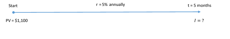


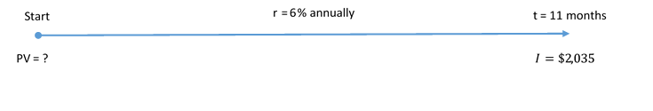


 or
or  of a year. However, if you use the exact number of days, the 31 days in July and 31 days in August total 62 days. In a 365-day year that is
  or t = 0.169863 of a year. Notice a difference of 0.003196 (0.169863 – 0.16) occurs. Therefore, to be precise in performing simple interest calculations, you must calculate the exact number of days involved in the transaction.

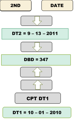

}")


\\ &=\$10,\!000 \times \left(0.07 \times \frac{11}{12}\right)\\ &=\$10,\!641.67 \end{align}")
 per year
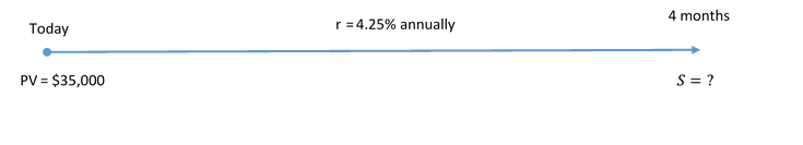
\\ &=\$35,\!000 \times \left(1+4\frac{1}{4}\% \times \frac{4}{12}\right)\\ &=\$35,\!000 \times (1+0.0425 \times 0.\overline{3})\\ &=\$35,\!495.83 \end{align}")
 that you must invest such that it will earn interest and end up at the $8,000 required for the tuition.
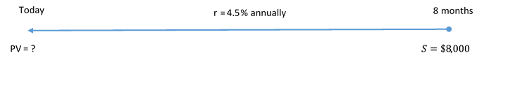
}\\ &=\frac{\$8,\!000}{(1+0.045 \times 0.\overline{6})}\\ &=\$7,\!766.99 \end{align}")


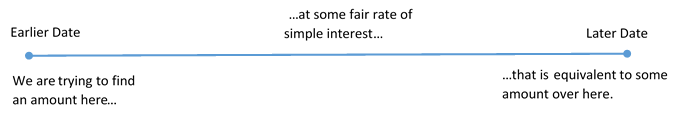

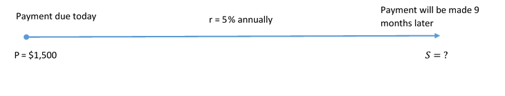
\\ S&=\$1,\!500 \times \left(1+5\% \times \frac{9}{12}\right)\\ &=\$1,\!500 \times (1+0.05 \times 0.75)\\ &=\$1,\!556.25 \end{align}")
 ).
).
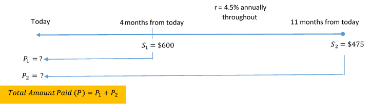
}\\ &=\$586.32 \end{align}")
}\\ &=\$446.36 \end{align}")


\left(\frac{4}{365}\right)=\$0.117808")

\left(\frac{7}{365}\right)=\$0.239726")
\left(\frac{7}{365}\right)=\$0.455479")

\left(\frac{7}{365}\right)=\$0.258904")


\left(\frac{14}{365}\right)=\$0.479452")

\left(\frac{14}{365}\right)=\$0.455479")

\left(\frac{3}{365}\right)=\$0.030821")

 and
and 
\left(\frac{364}{365}\right)\right)=\$10,\!074.79")
\left(\frac{182}{365}\right)\right)=\$10,\!034.90")
\left(\frac{182}{365}\right)\right)=\$10,\!069.93")
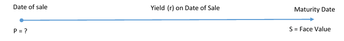
\left(\frac{182}{365}\right)}\\ &=\$99,\!257.61 \end{align}")
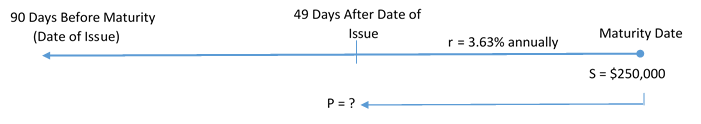
\left(\frac{41}{365}\right)}\\ &=\$248,\!984.76 \end{align}")
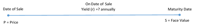
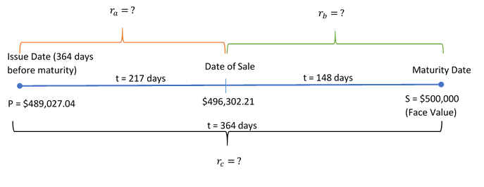
\left(\frac{217}{365}\right)}=2.50\% \end{align}")
\left(\frac{147}{365}\right)}=1.85\% \end{align}")
\left(\frac{364}{365}\right)}=2.25\% \end{align}")


")
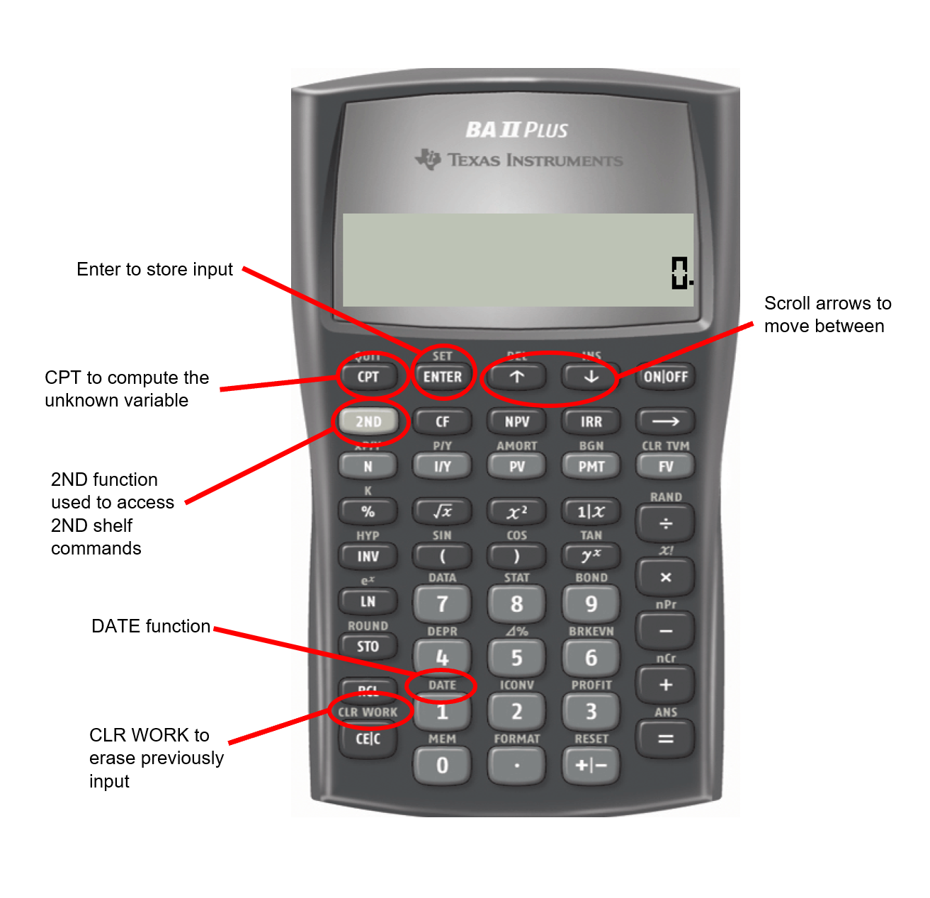
 and
and  to scroll through the display. The variables are:
}}{\text{Compounds per Year (C/Y)}}}")
 , for the following nominal interest rates:
}}{\text{Compounds per Year (C/Y)}}=\frac{9\%}{12}=0.75\%\;\text{per month}")
}}{\text{Compounds per Year (C/Y)}}=\frac{6\%}{4}=1.5\%\; \text{per quarter}")

 ;
; 
 per month is equal to a nominal interest rate of 7% compounded monthly.


\\ &=\$ 4,000+0.06(\$ 4,000)\\ &=\$ 4,000+\$ 240=\$ 4,240 \end{align} \nonumber")
") can be factored and rewritten as
can be factored and rewritten as ") .
.")
 =$4,200(1 + 0.06) = $4,240(1.06) = $4,494.40")
 is the result of the previous calculation where
  = $4,240") , the following algebraic substitution is possible:
, the following algebraic substitution is possible:(1 + i) = $4,000(1.06)(1.06) = $4200(1.06) = $4,494.40")
(1 + i) = PV(1 +i)^2")
")
}}")
 Value:}\;FV=PV \times (1+i)^n}")
 .
.}}{\text{Compounds per Year (C/Y)}}")
}")
^n")
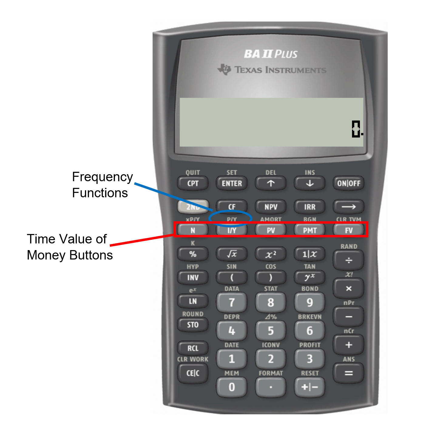
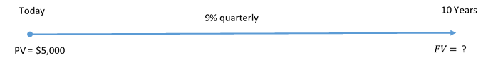

=4 \times 10=40")
^{40}=\$12,\!175.94")

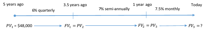

=4 \times 1.5=6")
^n\\ &= \$48,\!000 (1 + 0.015)^6\\ &= \$24,\!500(1.015)^6\\ &= \$52,\!485.27667 \end{align}")

= 2 \times 2.5=5")
^n\\ &= \$52,\!485.27667 (1+0.035)^5\\ &= \$62,\!336.04435 \end{align}")

= 12 \times 1=12")
^n\\ &= \$62,\!336.04435 (1+0.00325)^{12}\\ &= \$67,\!175.35 \end{align}")
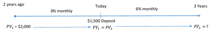

=12 \times 2=24")
^n\\ &= \$2,\!000 (1 + 0.005)^24\\ &= \$2,\!000(1.005)^24\\ &= \$2,\!254.319552 \end{align}")
}= 12 \times 3=36")
^n\\ &= \$3,\!754.319552 (1+0.005)^{36}\\ &= \$4,\!492.72 \end{align}")
:}\; PV=\frac{FV}{(1+i)^n}}")
")
^n}\end{align}")
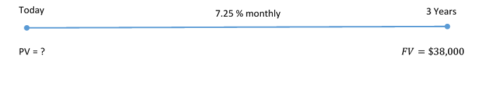

=3 \times 12=36")
^n}\\ &=\frac{38,\!000}{(1+0.006041\overline{6})^{36}}\\ &=30,\!592.06 \end{align}")
 key, then store the unrounded number back into the future value button by pressing FV. Change the N, I/Y, and C/Y as required for the next segment.
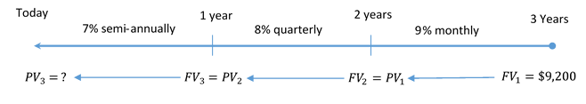

=1 \times 12=12")
^n}\\ &=\frac{9,\!200}{(1+0.0075)^{12}}\\ &=8,\!410.991026 \end{align}")

= 1 \times 4=4")
^n}\\ &=\frac{8,\!410.991026}{(1+0.02)^{4}}\\ &=7,\!770.455587 \end{align}")
= 1 \times 2=2")
^n}\\ &=\frac{7,\!770.455587}{(1+0.035)^{2}}\\ &=7,\!253.80 \end{align}")
{n_1}\times (1+i_2)^{n_2}\times (1+i_3)^{n_3}\times \ldots(1+i_n)^{n_n}}")

^{12}\times (1+0.02)^{4}\times (1+0.035)^{2}}=\$7,\!253.80")
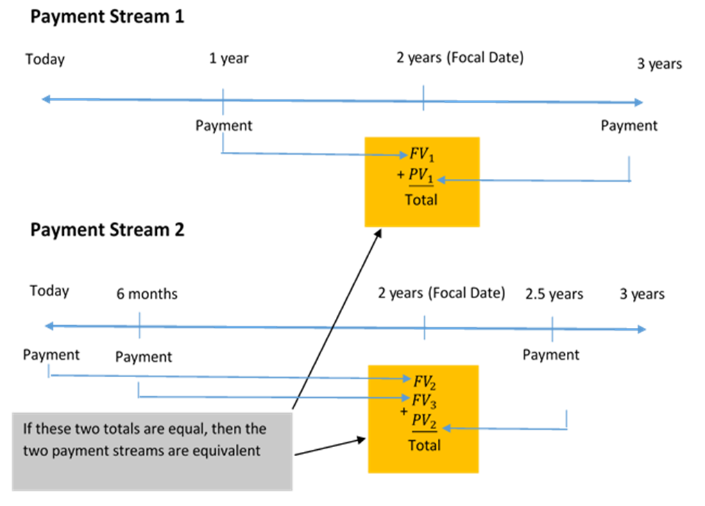
}}{\text{Compound per Year (C/Y)}}")
 \times (\text{Number of Years})")
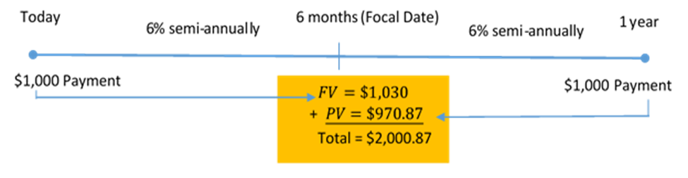
 .
.=2\times\frac{1}{2}=1") .
.^1=\$1,\!030") .
.^1}=\$970.87\end{align}") .
.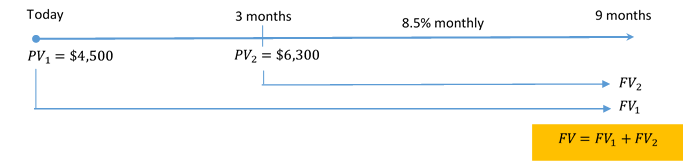
 .
.=12\times\frac{9}{12}=9") .
.=12\times\frac{6}{12}=6") .
.^9=\$4,\!795.138902") .
.^6=\$6,\!572.536425") .
.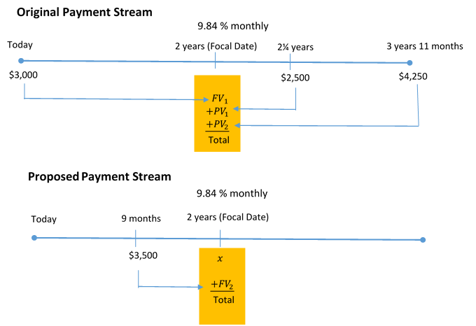
}}{\text{Compounds per Year (C/Y)}}=\frac{9.84\%}{12}=0.82\%\;\text{or}\;0.0082")
") .
. ;
; ^{24}=\$3,\!649.571607")
 ;
; 
 ;
; 
 ;
; ^{15}=\$3,\!956.110749")

}") .
.^{\frac{1}{n}}-1")
 rearrange, and solve for the nominal interest rate, I/Y.
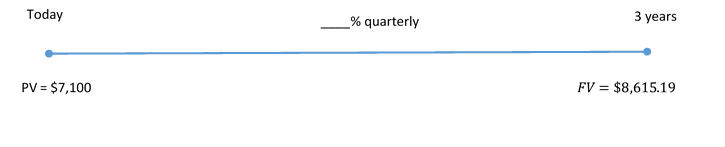
}=4 \times 3=12")
^n\\ \$8,\!615.19&=\$7,\!100(1+i)^{12}\\ 1.213407&=(1+i)^{12}\\ 1.213407^{\frac{1}{12}}&=1+i\\ 1.01624996&=1+i\\ i&=0.01624996 \end{align}")
} \end{align}")
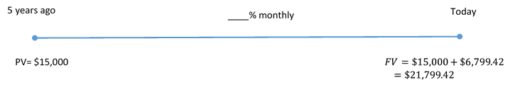
}=12 \times 5=60")
^n\\ \$21,\!799.42&=\$15,\!000(1+i)^{60}\\ 1.453294&=(1+i)^{60}\\ 1.453294^{\frac{1}{60}}&=1+i\\ 1.00625&=1+i\\ i&=0.00625 \end{align}")
} \end{align}")
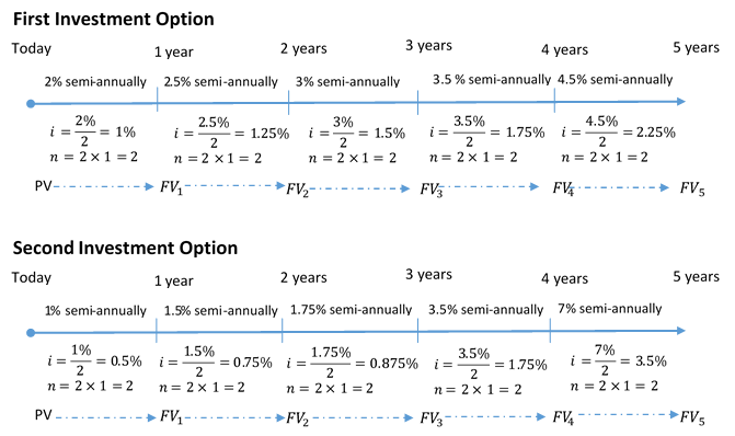

^{n_1} \times (1+i_2)^{n_2}\times \cdots \times (1+i_5)^{n_5}")
^{2} (1+0.0125)^{2}(1+0.015)^2(1+0.0175)^2(1+0.0225)^2\\ &=\$11,\!661.65972 \end{align}")
^{2} (1+0.0075)^{2}(1+0.00875)^2(1+0.0175)^2(1+0.035)^2\\ &=\$11,\!570.14666 \end{align}")

^{10}\\ 1.166165&=(1+i)^{10}\\ 1.166165^{\frac{1}{10}}&=1+i\\ 1.001549&=1+i\\ i&=0.001549 \end{align}")
^{10}\\ 1.157014&=(1+i)^{10}\\ 1.157015^{\frac{1}{10}}&=1+i\\ 1.014691&=1+i\\ i&=0.014691 \end{align}")


^{\frac{C/Y_{\text{Old}}}{C/Y _{\text{New}}}}-1 }")

^{\frac{C/Y_{\text{Old}}}{C/Y _{\text{New}}}}-1")


^{\frac{2}{1}}−1\\ &=6.7089 \end{align}")
^{\frac{4}{1}}−1\\ &=6.7336\end{align}")

}")


^{\frac{C/Y_{\text{Old}}}{C/Y _{\text{New}}}}-1\\ &=(1+0.00458\overline{3})^{\frac{12}{1}}-1\\ &=0.056408\;\text{or}\;5.6408\% \end{align}")
^{\frac{C/Y_{\text{Old}}}{C/Y _{\text{New}}}}-1\\ 0.0865&=(1+i_{\text{Old}})^{\frac{12}{1}}-1\\ 1.0865&=(1+i_{\text{Old}})^{12}\\ 1.0865^{\frac{1}{12}}&=1+i_{\text{Old}}\\ 1.006937&=1+i_{\text{Old}}\\ i_{\text{Old}}&=0.006937 \end{align}")

 ,
, 
^{\frac{C/Y_{\text{Old}}}{C/Y _{\text{New}}}}-1\\ &=(1+0.016425)^{\frac{4}{2}}-1\\ &=0.033119 \end{align}")


^{\frac{C/Y_{\text{Old}}}{C/Y _{\text{New}}}}-1\\ &=(1+0.01925)^{\frac{4}{2}}-1\\ &=0.038870 \end{align}")

 .
.
^n\\ \$67,\!113.46&=\$43,\!000(1+0.016625)^n\\ 1.560778&=1.016625^n\\ \ln(1.560778)&=\ln(1.016625)^n\;\text{(by taking ln of both sides)}\\ \ln(1.560778)&=n \ln(1.016625)\; \text{(by using the property} \ln(x)^n=n\ln(x))\\ n&=\frac{\ln(1.560778)}{\ln(1.016625)}\\ n&=\frac{0.445184}{0.016488}\\ n&=26.99996\;\text{or}\; 27\;\text{quarterly compounds} \end{align}")

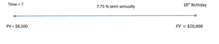

^n\\ \$20,\!000&=\$8,\!500(1+0.03875)^n\\ 2.352941&=1.03875^n\\ \ln(2.352941)&=\ln(1.03875)^n\;\text{(by taking ln of both sides)}\\ \ln(2.352941)&=n \ln(1.03875)\; \text{(by using the property} \ln(x)^n=n\ln(x))\\ n&=\frac{\ln(2.352941)}{\ln(1.03875)}\\ n&=\frac{0.855666}{0.038018}\\ n&=22.506828\;\text{semi-annual compounds} \end{align}")


}")
^{\frac{C/Y_{\text{Old}}}{C/Y_{New}}}-1")
 term in the formula. There is also no future value to calculate, just an interest amount. This changes

 = $5, and in the second year I = 1,000
  = $2.
= $2.

=2 \times 4=8")
 .
.^{n_1}(1+i_2)^{n_2} (1+i_3)^{n_3} \ldots")
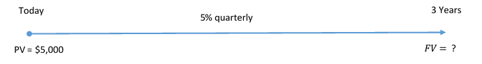

}=4 \times 3 =12")
^n\\ &=\$5,\!000(1+0.0125)^{12}\\ &=\$5,\!803.77 \end{align}")
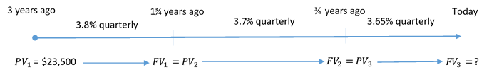

 years
years


^5=\$24,\!637.66119")
^4=\$25,\!561.98119")
^3=\$26,\!268.15")
^{n_1}(1+i_2)^{n_2} (1+i_3)^{n_3} \\ &=\$23,\!500(1+0.0095)^5(1+0.00925)^4(1+0.009125)^3\\ &=\$26,\!268.15 \end{align}")
}=4 \times 3=12")
^n\\ \$26,\!268.15&=\$23,\!500(1+i)^{12}\\ 1.117793&=(1+i)^{12}\\ 1.117793^{\frac{1}{12}}&=1+i\\ 1.009322&=1+i\\ i&=0.00932 \end{align}")

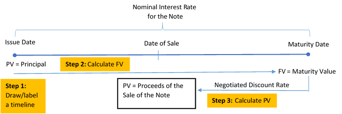
^n} \end{align}")
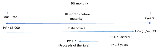

}=12 \times 3 =36")
^{36}=\$6,\!543.23")

}=4 \times 1.5 =36")
^n}\\ &=\frac{\$6,\!543.23}{(1+0.04)^6}\\ &=\$5,\!171.21 \end{align}")
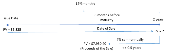


^{24}=\$8,\!665.94")
}=2 \times 0.5 =1")
^n\\ \$8,\!665.94&=\$7,\!950.40{(1+i)^1}\\ 1.090000&=1+i\\ i&=0.090000 \end{align}")

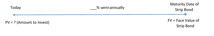
}}{\text{Compoundings per Year (C/Y)}}")
^n}\end{align}")

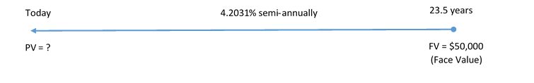

}=2 \times 23.5=47")
^n}\\ &=\frac{\$50,\!000}{(1+0.0210155)^{47}}\\ &=\$18,\!812.66 \end{align}")

}=2 \times 5=10")
^n\\ \$15,\!539.94&=\$10,\!772.52(1+i)^{10}\\ 1.442554&=(1+i){10}\\ 1.442554^{\frac{1}{10}}&=1+i\\ 1.037321&=1+i\\ i&=0.037321 \end{align}")


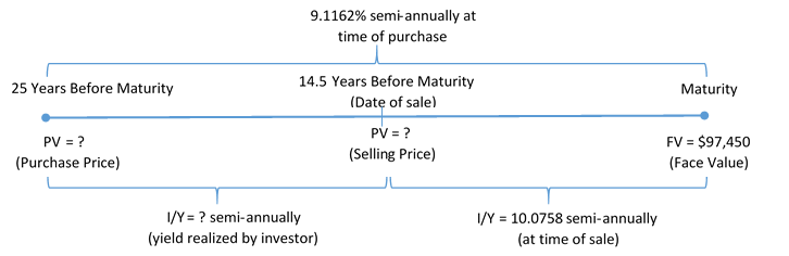

}=2 \times 25=50")
^{50}}\\ &=\$10,\!492.95 \end{align}")

}=2 \times 14.5=29")
^{29}}\\ &=\$23,\!428.63 \end{align}")
}=2 \times 10.5=21")
^n\\ \$23,\!428.63&=\$10,\!492.95(1+i)^{21}\\ 2.232797&=(1+i){21}\\ 2.232797^{\frac{1}{21}}&=1+i\\ 1.038991&=1+i\\ i&=0.038991 \end{align}")


![\colorbox{LightGray}{Formula 11.2A}\; \color{BlueViolet}{\text{Ordinary Annuity Future Value:}\; FV_{ORD}=PMT \left[\frac{(1+i)^n-1}{i}\right]}](https://jin71j2ebb.execute-api.ca-central-1.amazonaws.com/latest/latex?latex=%5Ccolorbox%7BLightGray%7D%7BFormula%2011.2A%7D%5C%3B%20%20%5Ccolor%7BBlueViolet%7D%7B%5Ctext%7BOrdinary%20Annuity%20Future%20Value%3A%7D%5C%3B%20FV_%7BORD%7D%3DPMT%20%5Cleft%5B%5Cfrac%7B%281%2Bi%29%5En-1%7D%7Bi%7D%5Cright%5D%7D&fg=000000&font=TeX&svg=1 "\colorbox{LightGray}{Formula 11.2A}\; \color{BlueViolet}{\text{Ordinary Annuity Future Value:}\; FV_{ORD}=PMT \left[\frac{(1+i)^n-1}{i}\right]}")
 C/Y) you need to calculate the equivalent periodic rate (ieq) per payment interval using the formula
^{\frac{C/Y}{P/Y}}-1")
![FV_{ORD}=PMT \left[\frac{(1+i_{eq})^n-1}{i_{eq}}\right]](https://jin71j2ebb.execute-api.ca-central-1.amazonaws.com/latest/latex?latex=FV_%7BORD%7D%3DPMT%20%5Cleft%5B%5Cfrac%7B%281%2Bi_%7Beq%7D%29%5En-1%7D%7Bi_%7Beq%7D%7D%5Cright%5D&fg=000000&font=TeX&svg=1 "FV_{ORD}=PMT \left[\frac{(1+i_{eq})^n-1}{i_{eq}}\right]")
}")
}=PV(1+i)^n")
")
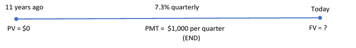

![\begin{align} FV_{ORD}&=PMT \left[ \frac{(1+i)^n-1}{i}\right]\\ &=\$1,\!000 \left[ \frac{(1+0.01825)^{44}-1}{0.01825}\right]\\ &=\$66,\!637.03 \end{align}](https://jin71j2ebb.execute-api.ca-central-1.amazonaws.com/latest/latex?latex=%5Cbegin%7Balign%7D%20%20FV_%7BORD%7D%26%3DPMT%20%5Cleft%5B%20%5Cfrac%7B%281%2Bi%29%5En-1%7D%7Bi%7D%5Cright%5D%5C%5C%20%20%26%3D%5C%241%2C%5C%21000%20%5Cleft%5B%20%5Cfrac%7B%281%2B0.01825%29%5E%7B44%7D-1%7D%7B0.01825%7D%5Cright%5D%5C%5C%20%20%26%3D%5C%2466%2C%5C%21637.03%20%20%5Cend%7Balign%7D&fg=000000&font=TeX&svg=1 "\begin{align} FV_{ORD}&=PMT \left[ \frac{(1+i)^n-1}{i}\right]\\ &=\$1,\!000 \left[ \frac{(1+0.01825)^{44}-1}{0.01825}\right]\\ &=\$66,\!637.03 \end{align}")
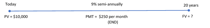

^{\frac{C/Y}{P/Y}}-1=(1+0.045)^{\frac{2}{12}}-1=0.007363123")
^{240}=\$58,\!163.64538")
![\begin{align} FV_{ORD}&=PMT \left[ \frac{(1+i_{eq})^n-1}{i_{eq}}\right]\\ &=\$250 \left[ \frac{(1+0.007363123)^{240}-1}{0.007363123}\right]\\ &=\$163,\!529.9486 \end{align}](https://jin71j2ebb.execute-api.ca-central-1.amazonaws.com/latest/latex?latex=%5Cbegin%7Balign%7D%20%20FV_%7BORD%7D%26%3DPMT%20%5Cleft%5B%20%5Cfrac%7B%281%2Bi_%7Beq%7D%29%5En-1%7D%7Bi_%7Beq%7D%7D%5Cright%5D%5C%5C%20%20%26%3D%5C%24250%20%5Cleft%5B%20%5Cfrac%7B%281%2B0.007363123%29%5E%7B240%7D-1%7D%7B0.007363123%7D%5Cright%5D%5C%5C%20%20%26%3D%5C%24163%2C%5C%21529.9486%20%20%5Cend%7Balign%7D&fg=000000&font=TeX&svg=1 "\begin{align} FV_{ORD}&=PMT \left[ \frac{(1+i_{eq})^n-1}{i_{eq}}\right]\\ &=\$250 \left[ \frac{(1+0.007363123)^{240}-1}{0.007363123}\right]\\ &=\$163,\!529.9486 \end{align}")
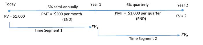

^{\frac{C/Y}{P/Y}}-1=(1+0.025)^{\frac{2}{12}}-1=0.004123915")
}=\$1,\!000(1+0.004123915)^{12}=\$1,\!050.625")
![\begin{align} FV_{ORD_1}&=PMT \left[ \frac{(1+i_{eq})^n-1}{i_{eq}}\right]\\ &=\$300 \left[ \frac{(1+0.004123915)^{12}-1}{0.004123915}\right]\\ &=\$3,\!682.786451 \end{align}](https://jin71j2ebb.execute-api.ca-central-1.amazonaws.com/latest/latex?latex=%5Cbegin%7Balign%7D%20%20FV_%7BORD_1%7D%26%3DPMT%20%5Cleft%5B%20%5Cfrac%7B%281%2Bi_%7Beq%7D%29%5En-1%7D%7Bi_%7Beq%7D%7D%5Cright%5D%5C%5C%20%20%26%3D%5C%24300%20%5Cleft%5B%20%5Cfrac%7B%281%2B0.004123915%29%5E%7B12%7D-1%7D%7B0.004123915%7D%5Cright%5D%5C%5C%20%20%26%3D%5C%243%2C%5C%21682.786451%20%20%5Cend%7Balign%7D&fg=000000&font=TeX&svg=1 "\begin{align} FV_{ORD_1}&=PMT \left[ \frac{(1+i_{eq})^n-1}{i_{eq}}\right]\\ &=\$300 \left[ \frac{(1+0.004123915)^{12}-1}{0.004123915}\right]\\ &=\$3,\!682.786451 \end{align}")
}=PV(1+i)^n=\$4,\!733.411442(1+0.015)^{4}=\$5,\!023.870384")
![\begin{align} FV_{ORD_2}&=PMT \left[ \frac{(1+i)^n-1}{i}\right]\\ &=\$1,\!000 \left[ \frac{(1+0.015)^{4}-1}{0.015}\right]\\ &=\$4,\!090.903375 \end{align}](https://jin71j2ebb.execute-api.ca-central-1.amazonaws.com/latest/latex?latex=%5Cbegin%7Balign%7D%20%20FV_%7BORD_2%7D%26%3DPMT%20%5Cleft%5B%20%5Cfrac%7B%281%2Bi%29%5En-1%7D%7Bi%7D%5Cright%5D%5C%5C%20%20%26%3D%5C%241%2C%5C%21000%20%5Cleft%5B%20%5Cfrac%7B%281%2B0.015%29%5E%7B4%7D-1%7D%7B0.015%7D%5Cright%5D%5C%5C%20%20%26%3D%5C%244%2C%5C%21090.903375%20%20%5Cend%7Balign%7D&fg=000000&font=TeX&svg=1 "\begin{align} FV_{ORD_2}&=PMT \left[ \frac{(1+i)^n-1}{i}\right]\\ &=\$1,\!000 \left[ \frac{(1+0.015)^{4}-1}{0.015}\right]\\ &=\$4,\!090.903375 \end{align}")
![\colorbox{LightGray}{Formula 11.2B}\; \color{BlueViolet}{\text{Annuity Due Future Value:}\; FV_{DUE}=PMT \left[\frac{(1+i)^n-1}{i}\right]\times(1+i)}](https://jin71j2ebb.execute-api.ca-central-1.amazonaws.com/latest/latex?latex=%5Ccolorbox%7BLightGray%7D%7BFormula%2011.2B%7D%5C%3B%20%20%5Ccolor%7BBlueViolet%7D%7B%5Ctext%7BAnnuity%20Due%20Future%20Value%3A%7D%5C%3B%20FV_%7BDUE%7D%3DPMT%20%5Cleft%5B%5Cfrac%7B%281%2Bi%29%5En-1%7D%7Bi%7D%5Cright%5D%5Ctimes%281%2Bi%29%7D&fg=000000&font=TeX&svg=1 "\colorbox{LightGray}{Formula 11.2B}\; \color{BlueViolet}{\text{Annuity Due Future Value:}\; FV_{DUE}=PMT \left[\frac{(1+i)^n-1}{i}\right]\times(1+i)}")
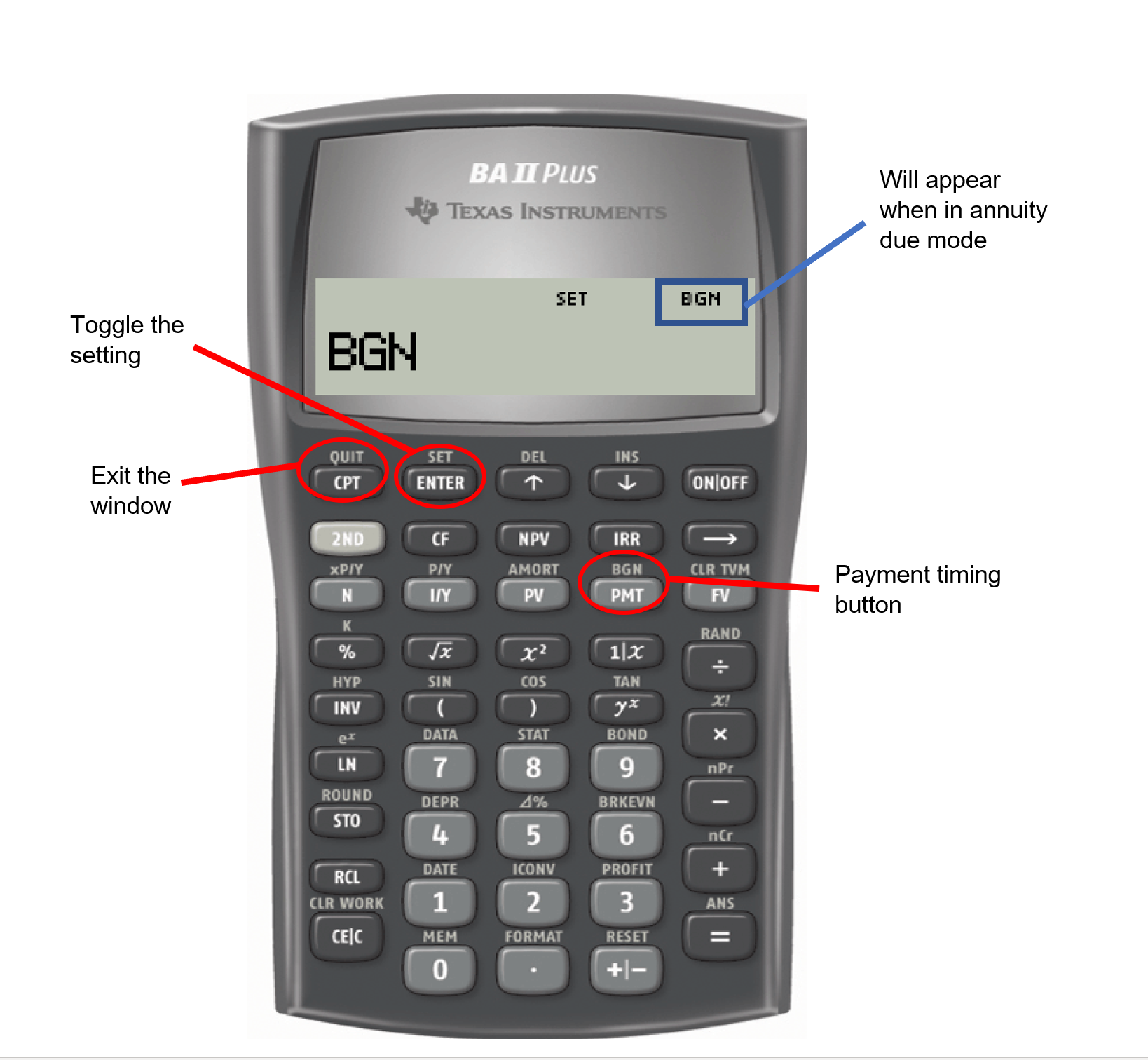
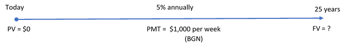

^{\frac{C/Y}{P/Y}}-1=(1+0.05)^{\frac{1}{52}}-1=0.000938713\;\text{per week}")
![\begin{align} FV_{DUE}&=PMT \left[ \frac{(1+i_{eq})^n-1}{i_{eq}}\right]\times(1+i_{eq})\\ &=\$1.\!000 \left[ \frac{(1+0.000938713)^{1300}-1}{0.000938713}\right](1+0.000938713)\\ &=\$2,\!544,\!543.218 \end{align}](https://jin71j2ebb.execute-api.ca-central-1.amazonaws.com/latest/latex?latex=%5Cbegin%7Balign%7D%20%20FV_%7BDUE%7D%26%3DPMT%20%5Cleft%5B%20%5Cfrac%7B%281%2Bi_%7Beq%7D%29%5En-1%7D%7Bi_%7Beq%7D%7D%5Cright%5D%5Ctimes%281%2Bi_%7Beq%7D%29%5C%5C%20%20%26%3D%5C%241.%5C%21000%20%5Cleft%5B%20%5Cfrac%7B%281%2B0.000938713%29%5E%7B1300%7D-1%7D%7B0.000938713%7D%5Cright%5D%281%2B0.000938713%29%5C%5C%20%20%26%3D%5C%242%2C%5C%21544%2C%5C%21543.218%20%20%5Cend%7Balign%7D&fg=000000&font=TeX&svg=1 "\begin{align} FV_{DUE}&=PMT \left[ \frac{(1+i_{eq})^n-1}{i_{eq}}\right]\times(1+i_{eq})\\ &=\$1.\!000 \left[ \frac{(1+0.000938713)^{1300}-1}{0.000938713}\right](1+0.000938713)\\ &=\$2,\!544,\!543.218 \end{align}")
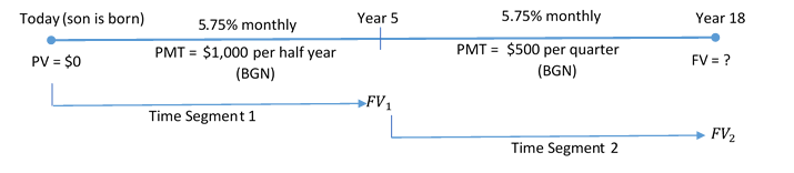

^{\frac{C/Y}{P/Y}}-1=(1+0.004719\overline{6})^{\frac{12}{2}}-1=0.029096609")
![\begin{align} FV_{DUE_1}&=PMT \left[ \frac{(1+i_{eq})^n-1}{i_{eq}}\right]\times(1+i_{eq})\\ &=\$1,\!000 \left[ \frac{(1+0.029096609)^{10}-1}{0.029096609}\right]\times(1+0.029096609)\\ &=\$11,\!748.47466=FV_1 \end{align}](https://jin71j2ebb.execute-api.ca-central-1.amazonaws.com/latest/latex?latex=%5Cbegin%7Balign%7D%20%20FV_%7BDUE_1%7D%26%3DPMT%20%5Cleft%5B%20%5Cfrac%7B%281%2Bi_%7Beq%7D%29%5En-1%7D%7Bi_%7Beq%7D%7D%5Cright%5D%5Ctimes%281%2Bi_%7Beq%7D%29%5C%5C%20%20%26%3D%5C%241%2C%5C%21000%20%5Cleft%5B%20%5Cfrac%7B%281%2B0.029096609%29%5E%7B10%7D-1%7D%7B0.029096609%7D%5Cright%5D%5Ctimes%281%2B0.029096609%29%5C%5C%20%20%26%3D%5C%2411%2C%5C%21748.47466%3DFV_1%20%20%5Cend%7Balign%7D&fg=000000&font=TeX&svg=1 "\begin{align} FV_{DUE_1}&=PMT \left[ \frac{(1+i_{eq})^n-1}{i_{eq}}\right]\times(1+i_{eq})\\ &=\$1,\!000 \left[ \frac{(1+0.029096609)^{10}-1}{0.029096609}\right]\times(1+0.029096609)\\ &=\$11,\!748.47466=FV_1 \end{align}")

^{\frac{C/Y}{P/Y}}-1=(1+0.004719\overline{6})^{\frac{12}{4}}-1=0.01444399")
}=PV(1+i_{eq})^n=\$11,\!748.47466(1+0.01444399)^{52}=\$24,\!765.17")
![\begin{align} FV_{DUE_2}&=PMT \left[ \frac{(1+i_{eq})^n-1}{i_{eq}}\right]\times(1+i_{eq})\\ &=\$500 \left[ \frac{(1+0.01444399)^{52}-1}{0.01444399}\right]\times(1+0.01444399)\\ &=\$38,\!907.21529 \end{align}](https://jin71j2ebb.execute-api.ca-central-1.amazonaws.com/latest/latex?latex=%5Cbegin%7Balign%7D%20%20FV_%7BDUE_2%7D%26%3DPMT%20%5Cleft%5B%20%5Cfrac%7B%281%2Bi_%7Beq%7D%29%5En-1%7D%7Bi_%7Beq%7D%7D%5Cright%5D%5Ctimes%281%2Bi_%7Beq%7D%29%5C%5C%20%20%26%3D%5C%24500%20%5Cleft%5B%20%5Cfrac%7B%281%2B0.01444399%29%5E%7B52%7D-1%7D%7B0.01444399%7D%5Cright%5D%5Ctimes%281%2B0.01444399%29%5C%5C%20%20%26%3D%5C%2438%2C%5C%21907.21529%20%20%5Cend%7Balign%7D&fg=000000&font=TeX&svg=1 "\begin{align} FV_{DUE_2}&=PMT \left[ \frac{(1+i_{eq})^n-1}{i_{eq}}\right]\times(1+i_{eq})\\ &=\$500 \left[ \frac{(1+0.01444399)^{52}-1}{0.01444399}\right]\times(1+0.01444399)\\ &=\$38,\!907.21529 \end{align}")
![\colorbox{LightGray}{Formula 11.3A}\; \color{BlueViolet}{\text{Ordinary Annuity Present Value:}\; PV_{ORD}=PMT \left[\frac{1-(1+i)^{-n}}{i}\right]}](https://jin71j2ebb.execute-api.ca-central-1.amazonaws.com/latest/latex?latex=%5Ccolorbox%7BLightGray%7D%7BFormula%2011.3A%7D%5C%3B%20%20%5Ccolor%7BBlueViolet%7D%7B%5Ctext%7BOrdinary%20Annuity%20Present%20Value%3A%7D%5C%3B%20PV_%7BORD%7D%3DPMT%20%5Cleft%5B%5Cfrac%7B1-%281%2Bi%29%5E%7B-n%7D%7D%7Bi%7D%5Cright%5D%7D&fg=000000&font=TeX&svg=1 "\colorbox{LightGray}{Formula 11.3A}\; \color{BlueViolet}{\text{Ordinary Annuity Present Value:}\; PV_{ORD}=PMT \left[\frac{1-(1+i)^{-n}}{i}\right]}")
![\colorbox{LightGray}{Formula 11.3B}\; \color{BlueViolet}{\text{Annuity Due Present Value:}\; PV_{DUE}=PMT \left[\frac{1-(1+i)^{-n}}{i}\right] \times(1+i)}](https://jin71j2ebb.execute-api.ca-central-1.amazonaws.com/latest/latex?latex=%5Ccolorbox%7BLightGray%7D%7BFormula%2011.3B%7D%5C%3B%20%20%5Ccolor%7BBlueViolet%7D%7B%5Ctext%7BAnnuity%20Due%20Present%20Value%3A%7D%5C%3B%20PV_%7BDUE%7D%3DPMT%20%5Cleft%5B%5Cfrac%7B1-%281%2Bi%29%5E%7B-n%7D%7D%7Bi%7D%5Cright%5D%20%5Ctimes%281%2Bi%29%7D&fg=000000&font=TeX&svg=1 "\colorbox{LightGray}{Formula 11.3B}\; \color{BlueViolet}{\text{Annuity Due Present Value:}\; PV_{DUE}=PMT \left[\frac{1-(1+i)^{-n}}{i}\right] \times(1+i)}")
^{\frac{C/Y}{P/Y}}-1")
![PV_{ORD}=PMT \left[\frac{1-(1+i_{eq})^{-n}}{i_{eq}}\right]](https://jin71j2ebb.execute-api.ca-central-1.amazonaws.com/latest/latex?latex=PV_%7BORD%7D%3DPMT%20%5Cleft%5B%5Cfrac%7B1-%281%2Bi_%7Beq%7D%29%5E%7B-n%7D%7D%7Bi_%7Beq%7D%7D%5Cright%5D&fg=000000&font=TeX&svg=1 "PV_{ORD}=PMT \left[\frac{1-(1+i_{eq})^{-n}}{i_{eq}}\right]")
![PV_{DUE}=PMT \left[\frac{1-(1+i_{eq})^{-n}}{i_{eq}}\right] \times(1+i_{eq})](https://jin71j2ebb.execute-api.ca-central-1.amazonaws.com/latest/latex?latex=PV_%7BDUE%7D%3DPMT%20%5Cleft%5B%5Cfrac%7B1-%281%2Bi_%7Beq%7D%29%5E%7B-n%7D%7D%7Bi_%7Beq%7D%7D%5Cright%5D%20%5Ctimes%281%2Bi_%7Beq%7D%29&fg=000000&font=TeX&svg=1 "PV_{DUE}=PMT \left[\frac{1-(1+i_{eq})^{-n}}{i_{eq}}\right] \times(1+i_{eq})")
^n}\end{align}")
-PV")
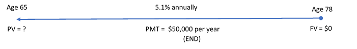

}=1 \times 13=13")
![\begin{align} PV_{ORD}&=PMT \left[\frac{1-(1+i)^{-n}}{i}\right]\\ &=\$50,\!000\left[\frac{1-(1+0.051)^{-13}}{0.051}\right]\\ &=\$50,\!000\left[\frac{0.476201}{0.051}\right]\\ &=\$466,\!863.69 \end{align}](https://jin71j2ebb.execute-api.ca-central-1.amazonaws.com/latest/latex?latex=%5Cbegin%7Balign%7D%20%20PV_%7BORD%7D%26%3DPMT%20%5Cleft%5B%5Cfrac%7B1-%281%2Bi%29%5E%7B-n%7D%7D%7Bi%7D%5Cright%5D%5C%5C%20%20%26%3D%5C%2450%2C%5C%21000%5Cleft%5B%5Cfrac%7B1-%281%2B0.051%29%5E%7B-13%7D%7D%7B0.051%7D%5Cright%5D%5C%5C%20%20%26%3D%5C%2450%2C%5C%21000%5Cleft%5B%5Cfrac%7B0.476201%7D%7B0.051%7D%5Cright%5D%5C%5C%20%20%26%3D%5C%24466%2C%5C%21863.69%20%20%5Cend%7Balign%7D&fg=000000&font=TeX&svg=1 "\begin{align} PV_{ORD}&=PMT \left[\frac{1-(1+i)^{-n}}{i}\right]\\ &=\$50,\!000\left[\frac{1-(1+0.051)^{-13}}{0.051}\right]\\ &=\$50,\!000\left[\frac{0.476201}{0.051}\right]\\ &=\$466,\!863.69 \end{align}")
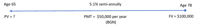

^{\frac{C/Y}{P/Y}}-1=(1+0.0255)^{\frac{2}{1}}-1=0.05165025\;\text{per year}")
}=1 \times 13=13")
^n}\\ &=\frac{\$100,\!000}{(1+0.05165025)^{13}}\\ &=\$51,\!960.42776 \end{align}")
![\begin{align} PV_{DUE}&=PMT \left[\frac{1-(1+i_{eq})^{-n}}{i_{eq}}\right] \times(1+i_{eq})\\ &=\$50,\!000 \left[\frac{1-(1+0.05165025)^{-13}}{0.05165025}\right] \times(1+0.05165025)\\ &=\$489,\!066.6372 \end{align}](https://jin71j2ebb.execute-api.ca-central-1.amazonaws.com/latest/latex?latex=%5Cbegin%7Balign%7D%20%20PV_%7BDUE%7D%26%3DPMT%20%5Cleft%5B%5Cfrac%7B1-%281%2Bi_%7Beq%7D%29%5E%7B-n%7D%7D%7Bi_%7Beq%7D%7D%5Cright%5D%20%5Ctimes%281%2Bi_%7Beq%7D%29%5C%5C%20%20%26%3D%5C%2450%2C%5C%21000%20%5Cleft%5B%5Cfrac%7B1-%281%2B0.05165025%29%5E%7B-13%7D%7D%7B0.05165025%7D%5Cright%5D%20%5Ctimes%281%2B0.05165025%29%5C%5C%20%20%26%3D%5C%24489%2C%5C%21066.6372%20%20%5Cend%7Balign%7D&fg=000000&font=TeX&svg=1 "\begin{align} PV_{DUE}&=PMT \left[\frac{1-(1+i_{eq})^{-n}}{i_{eq}}\right] \times(1+i_{eq})\\ &=\$50,\!000 \left[\frac{1-(1+0.05165025)^{-13}}{0.05165025}\right] \times(1+0.05165025)\\ &=\$489,\!066.6372 \end{align}")
-PV\\ &=(13 \times \$50,\!000+\$100,\!000)-\$541,\!027.07\\ &=\$750,\!000-\$541,\!027.07\\ &=\$208,\!972.93 \end{align}")
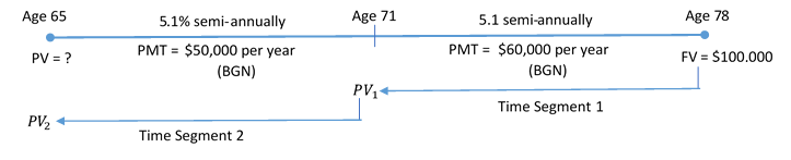
}=1 \times 7=7")
}&=\frac{FV}{(1+i_{eq})^n}\\ &=\frac{\$100,\!000}{(1+0.05165025)^{7}}\\ &=\$70,\!291.15736 \end{align}")
![\begin{align} PV_{DUE_1}&=PMT \left[\frac{1-(1+i_{eq})^{-n}}{i_{eq}}\right] \times(1+i_{eq})\\ &=\$60,\!000 \left[\frac{1-(1+0.05165025)^{-7}}{0.05165025}\right] \times(1+0.05165025)\\ &=\$362,\!940.8778 \end{align}](https://jin71j2ebb.execute-api.ca-central-1.amazonaws.com/latest/latex?latex=%5Cbegin%7Balign%7D%20%20PV_%7BDUE_1%7D%26%3DPMT%20%5Cleft%5B%5Cfrac%7B1-%281%2Bi_%7Beq%7D%29%5E%7B-n%7D%7D%7Bi_%7Beq%7D%7D%5Cright%5D%20%5Ctimes%281%2Bi_%7Beq%7D%29%5C%5C%20%20%26%3D%5C%2460%2C%5C%21000%20%5Cleft%5B%5Cfrac%7B1-%281%2B0.05165025%29%5E%7B-7%7D%7D%7B0.05165025%7D%5Cright%5D%20%5Ctimes%281%2B0.05165025%29%5C%5C%20%20%26%3D%5C%24362%2C%5C%21940.8778%20%20%5Cend%7Balign%7D&fg=000000&font=TeX&svg=1 "\begin{align} PV_{DUE_1}&=PMT \left[\frac{1-(1+i_{eq})^{-n}}{i_{eq}}\right] \times(1+i_{eq})\\ &=\$60,\!000 \left[\frac{1-(1+0.05165025)^{-7}}{0.05165025}\right] \times(1+0.05165025)\\ &=\$362,\!940.8778 \end{align}")
}=2 \times 6=6")
}&=\frac{FV_1}{(1+i_{eq})^n}\\ &=\frac{\$433,\!232.0352}{(1+0.05165025)^6}\\ &=\$320,\!252.5426 \end{align}")
![\begin{align} PV_{DUE_2}&=PMT \left[\frac{1-(1+i_{eq})^{-n}}{i_{eq}}\right] \times(1+i_{eq})\\ &=\$50,\!000 \left[\frac{1-(1+0.05165025)^{-6}}{0.05165025}\right] \times(1+0.05165025)\\ &=\$265,\!489.8749 \end{align}](https://jin71j2ebb.execute-api.ca-central-1.amazonaws.com/latest/latex?latex=%5Cbegin%7Balign%7D%20%20PV_%7BDUE_2%7D%26%3DPMT%20%5Cleft%5B%5Cfrac%7B1-%281%2Bi_%7Beq%7D%29%5E%7B-n%7D%7D%7Bi_%7Beq%7D%7D%5Cright%5D%20%5Ctimes%281%2Bi_%7Beq%7D%29%5C%5C%20%20%26%3D%5C%2450%2C%5C%21000%20%5Cleft%5B%5Cfrac%7B1-%281%2B0.05165025%29%5E%7B-6%7D%7D%7B0.05165025%7D%5Cright%5D%20%5Ctimes%281%2B0.05165025%29%5C%5C%20%20%26%3D%5C%24265%2C%5C%21489.8749%20%20%5Cend%7Balign%7D&fg=000000&font=TeX&svg=1 "\begin{align} PV_{DUE_2}&=PMT \left[\frac{1-(1+i_{eq})^{-n}}{i_{eq}}\right] \times(1+i_{eq})\\ &=\$50,\!000 \left[\frac{1-(1+0.05165025)^{-6}}{0.05165025}\right] \times(1+0.05165025)\\ &=\$265,\!489.8749 \end{align}")
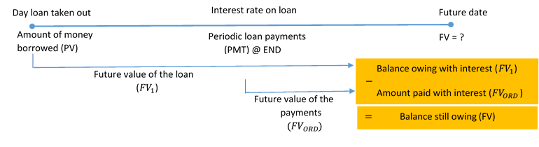
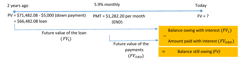

}=12 \times 2=24")
^n=\$66,\!482.08(1+0.00491\overline{6})^{24}=\$74,\!786.94231")
![\begin{align} FV_{ORD}&=PMT \left[ \frac{(1+i)^n-1}{i}\right]\\ &=\$1,\!282.20 \left[ \frac{(1+0.00491\overline{6})^{24}-1}{0.00491\overline{6}}\right]\\ &=\$32,\!577.13179 \end{align}](https://jin71j2ebb.execute-api.ca-central-1.amazonaws.com/latest/latex?latex=%5Cbegin%7Balign%7D%20%20FV_%7BORD%7D%26%3DPMT%20%5Cleft%5B%20%5Cfrac%7B%281%2Bi%29%5En-1%7D%7Bi%7D%5Cright%5D%5C%5C%20%20%26%3D%5C%241%2C%5C%21282.20%20%5Cleft%5B%20%5Cfrac%7B%281%2B0.00491%5Coverline%7B6%7D%29%5E%7B24%7D-1%7D%7B0.00491%5Coverline%7B6%7D%7D%5Cright%5D%5C%5C%20%20%26%3D%5C%2432%2C%5C%21577.13179%20%20%5Cend%7Balign%7D&fg=000000&font=TeX&svg=1 "\begin{align} FV_{ORD}&=PMT \left[ \frac{(1+i)^n-1}{i}\right]\\ &=\$1,\!282.20 \left[ \frac{(1+0.00491\overline{6})^{24}-1}{0.00491\overline{6}}\right]\\ &=\$32,\!577.13179 \end{align}")
-PV\\ &=(24 \times \$1,\!282.20+\$42,\!209.81)-\$66,\!482.08\\ &=\$72,\!982.61-\$66,\!482.08\\ &=\$6,\!500.53 \end{align}")
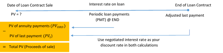
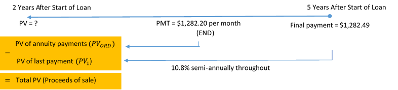

^{\frac{C/Y}{P/Y}}-1=(1+0.054)^{\frac{2}{12}}-1=0.008803937\;\text{per month}")
}=12 \times 3=36")
^n}\\ &=\frac{\$1,\!282.49}{(1+0.008803937)^{36}}\\ &=\$935.427906 \end{align}")
}=12 \times 3-1=35")
![\begin{align} PV_{ORD}&=PMT \left[\frac{1-(1+i_{eq})^{-n}}{i_{eq}}\right]\\ &=\$1,\!282.20\left[\frac{1-(1+0.008803937)^{-35}}{0.008803937}\right]\\ &=\$38,\!477.10711 \end{align}](https://jin71j2ebb.execute-api.ca-central-1.amazonaws.com/latest/latex?latex=%5Cbegin%7Balign%7D%20%20PV_%7BORD%7D%26%3DPMT%20%5Cleft%5B%5Cfrac%7B1-%281%2Bi_%7Beq%7D%29%5E%7B-n%7D%7D%7Bi_%7Beq%7D%7D%5Cright%5D%5C%5C%20%20%26%3D%5C%241%2C%5C%21282.20%5Cleft%5B%5Cfrac%7B1-%281%2B0.008803937%29%5E%7B-35%7D%7D%7B0.008803937%7D%5Cright%5D%5C%5C%20%20%26%3D%5C%2438%2C%5C%21477.10711%20%20%5Cend%7Balign%7D&fg=000000&font=TeX&svg=1 "\begin{align} PV_{ORD}&=PMT \left[\frac{1-(1+i_{eq})^{-n}}{i_{eq}}\right]\\ &=\$1,\!282.20\left[\frac{1-(1+0.008803937)^{-35}}{0.008803937}\right]\\ &=\$38,\!477.10711 \end{align}")


![\begin{align} PV_{ORD}&=PMT \left[\frac{1-(1+i)^{-n}}{i}\right]\\ \$25,\!000&=PMT\left[\frac{1-(1+0.0065)^{-36}}{0.0065}\right]\\ PMT&=\frac{\$25,\!000}{32.005957}=\$781.10 \end{align}](https://jin71j2ebb.execute-api.ca-central-1.amazonaws.com/latest/latex?latex=%5Cbegin%7Balign%7D%20%20PV_%7BORD%7D%26%3DPMT%20%5Cleft%5B%5Cfrac%7B1-%281%2Bi%29%5E%7B-n%7D%7D%7Bi%7D%5Cright%5D%5C%5C%20%20%5C%2425%2C%5C%21000%26%3DPMT%5Cleft%5B%5Cfrac%7B1-%281%2B0.0065%29%5E%7B-36%7D%7D%7B0.0065%7D%5Cright%5D%5C%5C%20%20PMT%26%3D%5Cfrac%7B%5C%2425%2C%5C%21000%7D%7B32.005957%7D%3D%5C%24781.10%20%20%5Cend%7Balign%7D&fg=000000&font=TeX&svg=1 "\begin{align} PV_{ORD}&=PMT \left[\frac{1-(1+i)^{-n}}{i}\right]\\ \$25,\!000&=PMT\left[\frac{1-(1+0.0065)^{-36}}{0.0065}\right]\\ PMT&=\frac{\$25,\!000}{32.005957}=\$781.10 \end{align}")
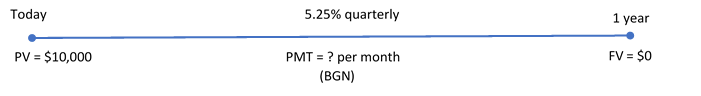

^{\frac{C/Y}{P/Y}}-1=(1+0.013125)^{\frac{4}{12}}-1=0.004355998\; \text{per month}")
}=12 \times 1=12")
![\begin{align} PV_{DUE}&=PMT \left[\frac{1-(1+i_{eq})^{-n}}{i_{eq}}\right] \times(1+i_{eq})\\ \$10,\!000&=PMT \left[\frac{1-(1+0.004355998)^{-12}}{0.004355998}\right] \times(1+0.004355998)\\ PMT&=\frac{\$10,\!000}{11.717849}=\$853.40 \end{align}](https://jin71j2ebb.execute-api.ca-central-1.amazonaws.com/latest/latex?latex=%5Cbegin%7Balign%7D%20%20PV_%7BDUE%7D%26%3DPMT%20%5Cleft%5B%5Cfrac%7B1-%281%2Bi_%7Beq%7D%29%5E%7B-n%7D%7D%7Bi_%7Beq%7D%7D%5Cright%5D%20%5Ctimes%281%2Bi_%7Beq%7D%29%5C%5C%20%20%5C%2410%2C%5C%21000%26%3DPMT%20%5Cleft%5B%5Cfrac%7B1-%281%2B0.004355998%29%5E%7B-12%7D%7D%7B0.004355998%7D%5Cright%5D%20%5Ctimes%281%2B0.004355998%29%5C%5C%20%20PMT%26%3D%5Cfrac%7B%5C%2410%2C%5C%21000%7D%7B11.717849%7D%3D%5C%24853.40%20%20%5Cend%7Balign%7D&fg=000000&font=TeX&svg=1 "\begin{align} PV_{DUE}&=PMT \left[\frac{1-(1+i_{eq})^{-n}}{i_{eq}}\right] \times(1+i_{eq})\\ \$10,\!000&=PMT \left[\frac{1-(1+0.004355998)^{-12}}{0.004355998}\right] \times(1+0.004355998)\\ PMT&=\frac{\$10,\!000}{11.717849}=\$853.40 \end{align}")
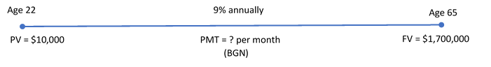

^{\frac{C/Y}{P/Y}}-1=(1+0.09)^{\frac{1}{12}}-1=0.007207323\; \text{per month}")
}=12 \times 43=516")
^n=\$10,\!000\times(1+0.007207323)^{516}=\$406,\!761.0984")

![\begin{align} FV_{DUE}&=PMT \left[ \frac{(1+i_{eq})^n-1}{i_{eq}}\right]\times(1+i_{eq})\\ \$1,\!293,\!238.902&=PMT \left[ \frac{(1+0.007207323)^{516}-1}{0.007207323}\right]\times(1+0.007207323)\\ PMT&=\frac{\$1,\!293,\!238.902}{5,\!544.647665}=\$233.24 \end{align}](https://jin71j2ebb.execute-api.ca-central-1.amazonaws.com/latest/latex?latex=%5Cbegin%7Balign%7D%20%20FV_%7BDUE%7D%26%3DPMT%20%5Cleft%5B%20%5Cfrac%7B%281%2Bi_%7Beq%7D%29%5En-1%7D%7Bi_%7Beq%7D%7D%5Cright%5D%5Ctimes%281%2Bi_%7Beq%7D%29%5C%5C%20%20%5C%241%2C%5C%21293%2C%5C%21238.902%26%3DPMT%20%5Cleft%5B%20%5Cfrac%7B%281%2B0.007207323%29%5E%7B516%7D-1%7D%7B0.007207323%7D%5Cright%5D%5Ctimes%281%2B0.007207323%29%5C%5C%20%20PMT%26%3D%5Cfrac%7B%5C%241%2C%5C%21293%2C%5C%21238.902%7D%7B5%2C%5C%21544.647665%7D%3D%5C%24233.24%20%20%5Cend%7Balign%7D&fg=000000&font=TeX&svg=1 "\begin{align} FV_{DUE}&=PMT \left[ \frac{(1+i_{eq})^n-1}{i_{eq}}\right]\times(1+i_{eq})\\ \$1,\!293,\!238.902&=PMT \left[ \frac{(1+0.007207323)^{516}-1}{0.007207323}\right]\times(1+0.007207323)\\ PMT&=\frac{\$1,\!293,\!238.902}{5,\!544.647665}=\$233.24 \end{align}")
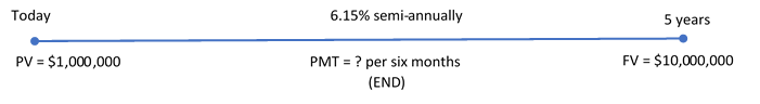

}=2 \times 5=10")
^n=\$1,000,\!000\times(1+0.03075)^{10}=\$1,\!353,\!734.306")

![\begin{align} FV_{ORD}&=PMT \left[\frac{(1+i)^n-1}{i}\right]\\ \$8,\!646,\!265.694&=PMT\left[\frac{(1+0.03075)^{10}-1}{0.03075}\right]\\ PMT&=\frac{\$8,\!646,\!265.694}{11.503554}=\$751,\!616.87 \end{align}](https://jin71j2ebb.execute-api.ca-central-1.amazonaws.com/latest/latex?latex=%5Cbegin%7Balign%7D%20%20FV_%7BORD%7D%26%3DPMT%20%5Cleft%5B%5Cfrac%7B%281%2Bi%29%5En-1%7D%7Bi%7D%5Cright%5D%5C%5C%20%20%5C%248%2C%5C%21646%2C%5C%21265.694%26%3DPMT%5Cleft%5B%5Cfrac%7B%281%2B0.03075%29%5E%7B10%7D-1%7D%7B0.03075%7D%5Cright%5D%5C%5C%20%20PMT%26%3D%5Cfrac%7B%5C%248%2C%5C%21646%2C%5C%21265.694%7D%7B11.503554%7D%3D%5C%24751%2C%5C%21616.87%20%20%5Cend%7Balign%7D&fg=000000&font=TeX&svg=1 "\begin{align} FV_{ORD}&=PMT \left[\frac{(1+i)^n-1}{i}\right]\\ \$8,\!646,\!265.694&=PMT\left[\frac{(1+0.03075)^{10}-1}{0.03075}\right]\\ PMT&=\frac{\$8,\!646,\!265.694}{11.503554}=\$751,\!616.87 \end{align}")


![\begin{align} PV_{DUE}&=PMT \left[\frac{1-(1+i)^{-n}}{i}\right] \times(1+i)\\ \$500,\!000&=\$3,\!000 \left[\frac{1-(1+0.004\overline{3})^{-n}}{0.004\overline{3}}\right]\times(1+0.004\overline{3})\\ 165.947560&=\frac{1-0.995685^n}{0.0043}\\ 0.995685^n&=0.280893\\ n\times \ln(0.995685)&=\ln(0.280893)\\ n&=\frac{-1.2697323}{-0.004323}\\ n&=293.660180 \end{align}](https://jin71j2ebb.execute-api.ca-central-1.amazonaws.com/latest/latex?latex=%5Cbegin%7Balign%7D%20%20PV_%7BDUE%7D%26%3DPMT%20%5Cleft%5B%5Cfrac%7B1-%281%2Bi%29%5E%7B-n%7D%7D%7Bi%7D%5Cright%5D%20%5Ctimes%281%2Bi%29%5C%5C%20%20%5C%24500%2C%5C%21000%26%3D%5C%243%2C%5C%21000%20%5Cleft%5B%5Cfrac%7B1-%281%2B0.004%5Coverline%7B3%7D%29%5E%7B-n%7D%7D%7B0.004%5Coverline%7B3%7D%7D%5Cright%5D%5Ctimes%281%2B0.004%5Coverline%7B3%7D%29%5C%5C%20%20165.947560%26%3D%5Cfrac%7B1-0.995685%5En%7D%7B0.0043%7D%5C%5C%20%200.995685%5En%26%3D0.280893%5C%5C%20%20n%5Ctimes%20%5Cln%280.995685%29%26%3D%5Cln%280.280893%29%5C%5C%20%20n%26%3D%5Cfrac%7B-1.2697323%7D%7B-0.004323%7D%5C%5C%20%20n%26%3D293.660180%20%20%5Cend%7Balign%7D&fg=000000&font=TeX&svg=1 "\begin{align} PV_{DUE}&=PMT \left[\frac{1-(1+i)^{-n}}{i}\right] \times(1+i)\\ \$500,\!000&=\$3,\!000 \left[\frac{1-(1+0.004\overline{3})^{-n}}{0.004\overline{3}}\right]\times(1+0.004\overline{3})\\ 165.947560&=\frac{1-0.995685^n}{0.0043}\\ 0.995685^n&=0.280893\\ n\times \ln(0.995685)&=\ln(0.280893)\\ n&=\frac{-1.2697323}{-0.004323}\\ n&=293.660180 \end{align}")


![\begin{align} PV_{ORD}&=PMT \left[\frac{1-(1+i)^{-n}}{i}\right]\\ \$47,\!604.41&=\$1,\!000 \left[\frac{1-(1+0.002)^{-n}}{0.002}\right]\\ 0.095208&=1-0.998003^n\\ 0.998003^n&=0.904791\\ n \times \ln(0.998003)&=\ln(0.904791)\\ n&=\frac{-0.100051}{-0.001998}\\ &=50.075560 \end{align}](https://jin71j2ebb.execute-api.ca-central-1.amazonaws.com/latest/latex?latex=%5Cbegin%7Balign%7D%20%20PV_%7BORD%7D%26%3DPMT%20%5Cleft%5B%5Cfrac%7B1-%281%2Bi%29%5E%7B-n%7D%7D%7Bi%7D%5Cright%5D%5C%5C%20%20%5C%2447%2C%5C%21604.41%26%3D%5C%241%2C%5C%21000%20%20%5Cleft%5B%5Cfrac%7B1-%281%2B0.002%29%5E%7B-n%7D%7D%7B0.002%7D%5Cright%5D%5C%5C%20%200.095208%26%3D1-0.998003%5En%5C%5C%20%200.998003%5En%26%3D0.904791%5C%5C%20%20n%20%5Ctimes%20%5Cln%280.998003%29%26%3D%5Cln%280.904791%29%5C%5C%20%20n%26%3D%5Cfrac%7B-0.100051%7D%7B-0.001998%7D%5C%5C%20%20%26%3D50.075560%20%20%5Cend%7Balign%7D&fg=000000&font=TeX&svg=1 "\begin{align} PV_{ORD}&=PMT \left[\frac{1-(1+i)^{-n}}{i}\right]\\ \$47,\!604.41&=\$1,\!000 \left[\frac{1-(1+0.002)^{-n}}{0.002}\right]\\ 0.095208&=1-0.998003^n\\ 0.998003^n&=0.904791\\ n \times \ln(0.998003)&=\ln(0.904791)\\ n&=\frac{-0.100051}{-0.001998}\\ &=50.075560 \end{align}")

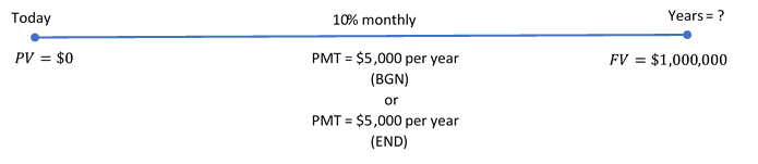

![\begin{align} FV_{ORD}&=PMT \left[\frac{(1+i)^n-1}{i}\right]\\ \$1,\!000,\!000&=\$5,\!000 \left[\frac{(1+0.008\overline{3})^n-1}{0.0088\overline{3}}\right]\\ 20.942613&=1.104713^n-1\\ 21.942613&=1.104713^n\\ \ln(21.942613)&=n \times\ln(1.104713)\\ n&=\frac{21.942613}{1.104713}\\ &=31.012812\; \text{or}\; 32\; \text{years} \end{align}](https://jin71j2ebb.execute-api.ca-central-1.amazonaws.com/latest/latex?latex=%5Cbegin%7Balign%7D%20%20FV_%7BORD%7D%26%3DPMT%20%5Cleft%5B%5Cfrac%7B%281%2Bi%29%5En-1%7D%7Bi%7D%5Cright%5D%5C%5C%20%20%5C%241%2C%5C%21000%2C%5C%21000%26%3D%5C%245%2C%5C%21000%20%5Cleft%5B%5Cfrac%7B%281%2B0.008%5Coverline%7B3%7D%29%5En-1%7D%7B0.0088%5Coverline%7B3%7D%7D%5Cright%5D%5C%5C%20%2020.942613%26%3D1.104713%5En-1%5C%5C%20%2021.942613%26%3D1.104713%5En%5C%5C%20%20%5Cln%2821.942613%29%26%3Dn%20%5Ctimes%5Cln%281.104713%29%5C%5C%20%20n%26%3D%5Cfrac%7B21.942613%7D%7B1.104713%7D%5C%5C%20%20%26%3D31.012812%5C%3B%20%5Ctext%7Bor%7D%5C%3B%2032%5C%3B%20%5Ctext%7Byears%7D%20%20%5Cend%7Balign%7D&fg=000000&font=TeX&svg=1 "\begin{align} FV_{ORD}&=PMT \left[\frac{(1+i)^n-1}{i}\right]\\ \$1,\!000,\!000&=\$5,\!000 \left[\frac{(1+0.008\overline{3})^n-1}{0.0088\overline{3}}\right]\\ 20.942613&=1.104713^n-1\\ 21.942613&=1.104713^n\\ \ln(21.942613)&=n \times\ln(1.104713)\\ n&=\frac{21.942613}{1.104713}\\ &=31.012812\; \text{or}\; 32\; \text{years} \end{align}")
![\begin{align} FV_{DUE}&=PMT \left[\frac{(1+i)^n-1}{i}\right]\times(1+i)\\ \$1,\!000,\!000&=\$5,\!000 \left[\frac{(1+0.0088\overline{3})^n-1}{0.0088\overline{3}}\right]\times(1+0.0088\overline{3})\\ 18.957514&=1.104713^n-1\\ 19.957514&=1.104713^n\\ \ln(19.957514)&=n\times\ln(1.104713)\\ n&=\frac{19.957514}{1.104713}\\ &=30.060618\; \text{or}\; 31\; \text{years} \end{align}](https://jin71j2ebb.execute-api.ca-central-1.amazonaws.com/latest/latex?latex=%5Cbegin%7Balign%7D%20%20FV_%7BDUE%7D%26%3DPMT%20%5Cleft%5B%5Cfrac%7B%281%2Bi%29%5En-1%7D%7Bi%7D%5Cright%5D%5Ctimes%281%2Bi%29%5C%5C%20%20%5C%241%2C%5C%21000%2C%5C%21000%26%3D%5C%245%2C%5C%21000%20%5Cleft%5B%5Cfrac%7B%281%2B0.0088%5Coverline%7B3%7D%29%5En-1%7D%7B0.0088%5Coverline%7B3%7D%7D%5Cright%5D%5Ctimes%281%2B0.0088%5Coverline%7B3%7D%29%5C%5C%20%2018.957514%26%3D1.104713%5En-1%5C%5C%20%2019.957514%26%3D1.104713%5En%5C%5C%20%20%5Cln%2819.957514%29%26%3Dn%5Ctimes%5Cln%281.104713%29%5C%5C%20%20n%26%3D%5Cfrac%7B19.957514%7D%7B1.104713%7D%5C%5C%20%20%26%3D30.060618%5C%3B%20%5Ctext%7Bor%7D%5C%3B%2031%5C%3B%20%5Ctext%7Byears%7D%20%20%5Cend%7Balign%7D&fg=000000&font=TeX&svg=1 "\begin{align} FV_{DUE}&=PMT \left[\frac{(1+i)^n-1}{i}\right]\times(1+i)\\ \$1,\!000,\!000&=\$5,\!000 \left[\frac{(1+0.0088\overline{3})^n-1}{0.0088\overline{3}}\right]\times(1+0.0088\overline{3})\\ 18.957514&=1.104713^n-1\\ 19.957514&=1.104713^n\\ \ln(19.957514)&=n\times\ln(1.104713)\\ n&=\frac{19.957514}{1.104713}\\ &=30.060618\; \text{or}\; 31\; \text{years} \end{align}")
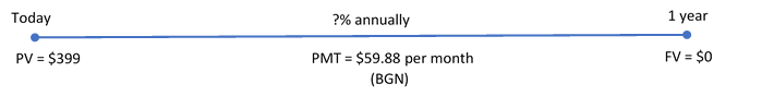
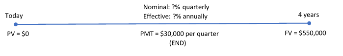
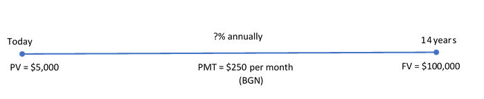
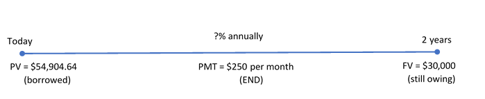


}")
![FV_{ORD}=PMT \left[\frac{(1+i)^n-1}{i}\right]](https://jin71j2ebb.execute-api.ca-central-1.amazonaws.com/latest/latex?latex=FV_%7BORD%7D%3DPMT%20%5Cleft%5B%5Cfrac%7B%281%2Bi%29%5En-1%7D%7Bi%7D%5Cright%5D&fg=000000&font=TeX&svg=1 "FV_{ORD}=PMT \left[\frac{(1+i)^n-1}{i}\right]")
![FV_{DUE}=PMT \left[\frac{(1+i)^n-1}{i}\right]\times(1+i)](https://jin71j2ebb.execute-api.ca-central-1.amazonaws.com/latest/latex?latex=FV_%7BDUE%7D%3DPMT%20%5Cleft%5B%5Cfrac%7B%281%2Bi%29%5En-1%7D%7Bi%7D%5Cright%5D%5Ctimes%281%2Bi%29&fg=000000&font=TeX&svg=1 "FV_{DUE}=PMT \left[\frac{(1+i)^n-1}{i}\right]\times(1+i)")
![PV_{ORD}=PMT \left[\frac{1-(1+i)^{-n}}{i}\right]](https://jin71j2ebb.execute-api.ca-central-1.amazonaws.com/latest/latex?latex=PV_%7BORD%7D%3DPMT%20%5Cleft%5B%5Cfrac%7B1-%281%2Bi%29%5E%7B-n%7D%7D%7Bi%7D%5Cright%5D&fg=000000&font=TeX&svg=1 "PV_{ORD}=PMT \left[\frac{1-(1+i)^{-n}}{i}\right]")
![PV_{DUE}=PMT \left[\frac{1-(1+i)^{-n}}{i}\right] \times(1+i)](https://jin71j2ebb.execute-api.ca-central-1.amazonaws.com/latest/latex?latex=PV_%7BDUE%7D%3DPMT%20%5Cleft%5B%5Cfrac%7B1-%281%2Bi%29%5E%7B-n%7D%7D%7Bi%7D%5Cright%5D%20%5Ctimes%281%2Bi%29&fg=000000&font=TeX&svg=1 "PV_{DUE}=PMT \left[\frac{1-(1+i)^{-n}}{i}\right] \times(1+i)")
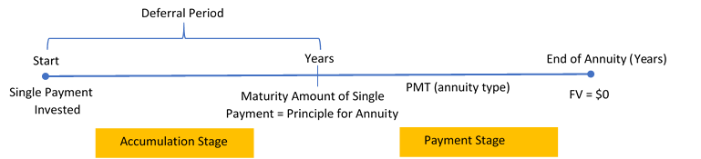
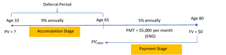
^{\frac{C/Y}{P/Y}}-1=(1+0.05)^{\frac{1}{12}}-1=0.004074124\;\text{per month}")
}=12 \times 15=180\;\text{payments}")
![\begin{align} PV_{ORD}&=PMT \left[\frac{1-(1+i)^{-n}}{i}\right]\\ &=\$5,\!000\left[\frac{1-(1+0.004074124)^{-180}}{0.004074124}\right]\\ &=\$5,\!000\left[\frac{0.518982921}{0.004074124}\right]\\ &=\$636,\!925.79 \end{align}](https://jin71j2ebb.execute-api.ca-central-1.amazonaws.com/latest/latex?latex=%5Cbegin%7Balign%7D%20%20PV_%7BORD%7D%26%3DPMT%20%5Cleft%5B%5Cfrac%7B1-%281%2Bi%29%5E%7B-n%7D%7D%7Bi%7D%5Cright%5D%5C%5C%20%20%26%3D%5C%245%2C%5C%21000%5Cleft%5B%5Cfrac%7B1-%281%2B0.004074124%29%5E%7B-180%7D%7D%7B0.004074124%7D%5Cright%5D%5C%5C%20%20%26%3D%5C%245%2C%5C%21000%5Cleft%5B%5Cfrac%7B0.518982921%7D%7B0.004074124%7D%5Cright%5D%5C%5C%20%20%26%3D%5C%24636%2C%5C%21925.79%20%20%5Cend%7Balign%7D&fg=000000&font=TeX&svg=1 "\begin{align} PV_{ORD}&=PMT \left[\frac{1-(1+i)^{-n}}{i}\right]\\ &=\$5,\!000\left[\frac{1-(1+0.004074124)^{-180}}{0.004074124}\right]\\ &=\$5,\!000\left[\frac{0.518982921}{0.004074124}\right]\\ &=\$636,\!925.79 \end{align}")

}=1 \times 32=32\;\text{compounds}")
^n}\\ &=\frac{\$636,\!925.79}{(1+0.09)^{32}}\\ &=\$40,\!405.54 \end{align}")
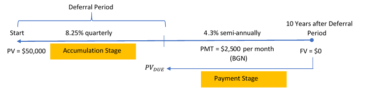

^{\frac{C/Y}{P/Y}}-1=(1+0.0205)^{\frac{2}{12}}-1=0.003551648\;\text{per month}")
}=12 \times 10=120\;\text{payments}")
![\begin{align} PV_{DUE}&=PMT \left[\frac{1-(1+i_{eq})^{-n}}{i_{eq}}\right] \times(1+i_{eq})\\ &=\$2,\!500 \left[\frac{1-(1+0.003551648)^{-120}}{0.003551648}\right] \times(1+0.003551648)\\ &=\$244,\!780.93 \end{align}](https://jin71j2ebb.execute-api.ca-central-1.amazonaws.com/latest/latex?latex=%5Cbegin%7Balign%7D%20%20PV_%7BDUE%7D%26%3DPMT%20%5Cleft%5B%5Cfrac%7B1-%281%2Bi_%7Beq%7D%29%5E%7B-n%7D%7D%7Bi_%7Beq%7D%7D%5Cright%5D%20%5Ctimes%281%2Bi_%7Beq%7D%29%5C%5C%20%20%26%3D%5C%242%2C%5C%21500%20%5Cleft%5B%5Cfrac%7B1-%281%2B0.003551648%29%5E%7B-120%7D%7D%7B0.003551648%7D%5Cright%5D%20%5Ctimes%281%2B0.003551648%29%5C%5C%20%20%26%3D%5C%24244%2C%5C%21780.93%20%20%5Cend%7Balign%7D&fg=000000&font=TeX&svg=1 "\begin{align} PV_{DUE}&=PMT \left[\frac{1-(1+i_{eq})^{-n}}{i_{eq}}\right] \times(1+i_{eq})\\ &=\$2,\!500 \left[\frac{1-(1+0.003551648)^{-120}}{0.003551648}\right] \times(1+0.003551648)\\ &=\$244,\!780.93 \end{align}")

^n\\ \$244,\!780.93&=\$50,\!000(1+0.020625)^n\\ 4.895618&=1.020625^n\\ \ln(4.85618)&=n \times \ln(1.020625)\\ n&=\frac{1.588340}{0.020415}\\ &=77.801923\;\text{quarterly compounds} \end{align}")


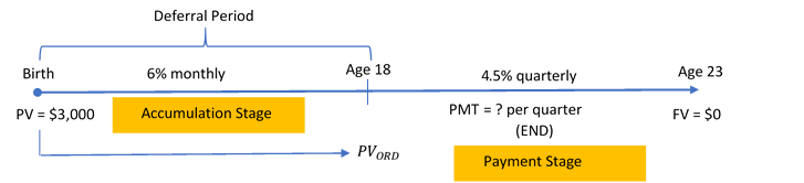
}=12 \times 18=216\;\text{compounds}")
^n\\ &=\$3,\!000(1+0.005)^{216}\\ &=\$8,\!810.30 \end{align}")

}=4 \times 5=20\;\text{payments}")
![\begin{align} PV_{ORD}&=PMT \left[\frac{1-(1+i)^{-n}}{i}\right]\\ \$8,\!810.30&=PMT\left[\frac{1-(1+0.01125)^{-20}}{0.01125}\right]\\ \$8,\!810.30&=PMT\left[\frac{0.200480}{0.01125}\right]\\ \$8,\!810.30&=PMT (17.820448)\\ PMT&=\frac{\$8,\!810.30}{17.820448}\\ &=\$494.39 \end{align}](https://jin71j2ebb.execute-api.ca-central-1.amazonaws.com/latest/latex?latex=%5Cbegin%7Balign%7D%20%20PV_%7BORD%7D%26%3DPMT%20%5Cleft%5B%5Cfrac%7B1-%281%2Bi%29%5E%7B-n%7D%7D%7Bi%7D%5Cright%5D%5C%5C%20%20%5C%248%2C%5C%21810.30%26%3DPMT%5Cleft%5B%5Cfrac%7B1-%281%2B0.01125%29%5E%7B-20%7D%7D%7B0.01125%7D%5Cright%5D%5C%5C%20%20%5C%248%2C%5C%21810.30%26%3DPMT%5Cleft%5B%5Cfrac%7B0.200480%7D%7B0.01125%7D%5Cright%5D%5C%5C%20%20%5C%248%2C%5C%21810.30%26%3DPMT%20%2817.820448%29%5C%5C%20%20PMT%26%3D%5Cfrac%7B%5C%248%2C%5C%21810.30%7D%7B17.820448%7D%5C%5C%20%20%26%3D%5C%24494.39%20%20%5Cend%7Balign%7D&fg=000000&font=TeX&svg=1 "\begin{align} PV_{ORD}&=PMT \left[\frac{1-(1+i)^{-n}}{i}\right]\\ \$8,\!810.30&=PMT\left[\frac{1-(1+0.01125)^{-20}}{0.01125}\right]\\ \$8,\!810.30&=PMT\left[\frac{0.200480}{0.01125}\right]\\ \$8,\!810.30&=PMT (17.820448)\\ PMT&=\frac{\$8,\!810.30}{17.820448}\\ &=\$494.39 \end{align}")
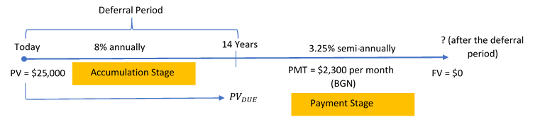

}=1 \times 14=14\;\text{compounds}")
^n\\ &=\$25,\!000(1+0.08)^{14}\\ &=\$73,\!429.84 \end{align}")

^{\frac{C/Y}{P/Y}}-1=(1+0.01625)^{\frac{2}{12}}-1=0.002690\;\text{per month}")
![\begin{align} PV_{DUE}&=PMT \left[\frac{1-(1+i_{eq})^{-n}}{i_{eq}}\right] \times(1+i_{eq})\\ 73,\!429.84&=\$2,\!300 \left[\frac{1-(1+0.002690)^{-n}}{0.002690}\right] \times(1+0.002690)\\ 31.840361&=\frac{1-0.997317^n}{0.002690}\\ 0.085656&=1-0.99730\\ \ln(0.997317)&=n \times \ln(0.914343)\\ n&=33.332019 =34\;\text{payments} \end{align}](https://jin71j2ebb.execute-api.ca-central-1.amazonaws.com/latest/latex?latex=%5Cbegin%7Balign%7D%20%20PV_%7BDUE%7D%26%3DPMT%20%5Cleft%5B%5Cfrac%7B1-%281%2Bi_%7Beq%7D%29%5E%7B-n%7D%7D%7Bi_%7Beq%7D%7D%5Cright%5D%20%5Ctimes%281%2Bi_%7Beq%7D%29%5C%5C%20%2073%2C%5C%21429.84%26%3D%5C%242%2C%5C%21300%20%5Cleft%5B%5Cfrac%7B1-%281%2B0.002690%29%5E%7B-n%7D%7D%7B0.002690%7D%5Cright%5D%20%5Ctimes%281%2B0.002690%29%5C%5C%20%2031.840361%26%3D%5Cfrac%7B1-0.997317%5En%7D%7B0.002690%7D%5C%5C%20%200.085656%26%3D1-0.99730%5C%5C%20%20%5Cln%280.997317%29%26%3Dn%20%5Ctimes%20%5Cln%280.914343%29%5C%5C%20%20n%26%3D33.332019%20%3D34%5C%3B%5Ctext%7Bpayments%7D%20%20%5Cend%7Balign%7D&fg=000000&font=TeX&svg=1 "\begin{align} PV_{DUE}&=PMT \left[\frac{1-(1+i_{eq})^{-n}}{i_{eq}}\right] \times(1+i_{eq})\\ 73,\!429.84&=\$2,\!300 \left[\frac{1-(1+0.002690)^{-n}}{0.002690}\right] \times(1+0.002690)\\ 31.840361&=\frac{1-0.997317^n}{0.002690}\\ 0.085656&=1-0.99730\\ \ln(0.997317)&=n \times \ln(0.914343)\\ n&=33.332019 =34\;\text{payments} \end{align}")


 , per payment interval using the formula
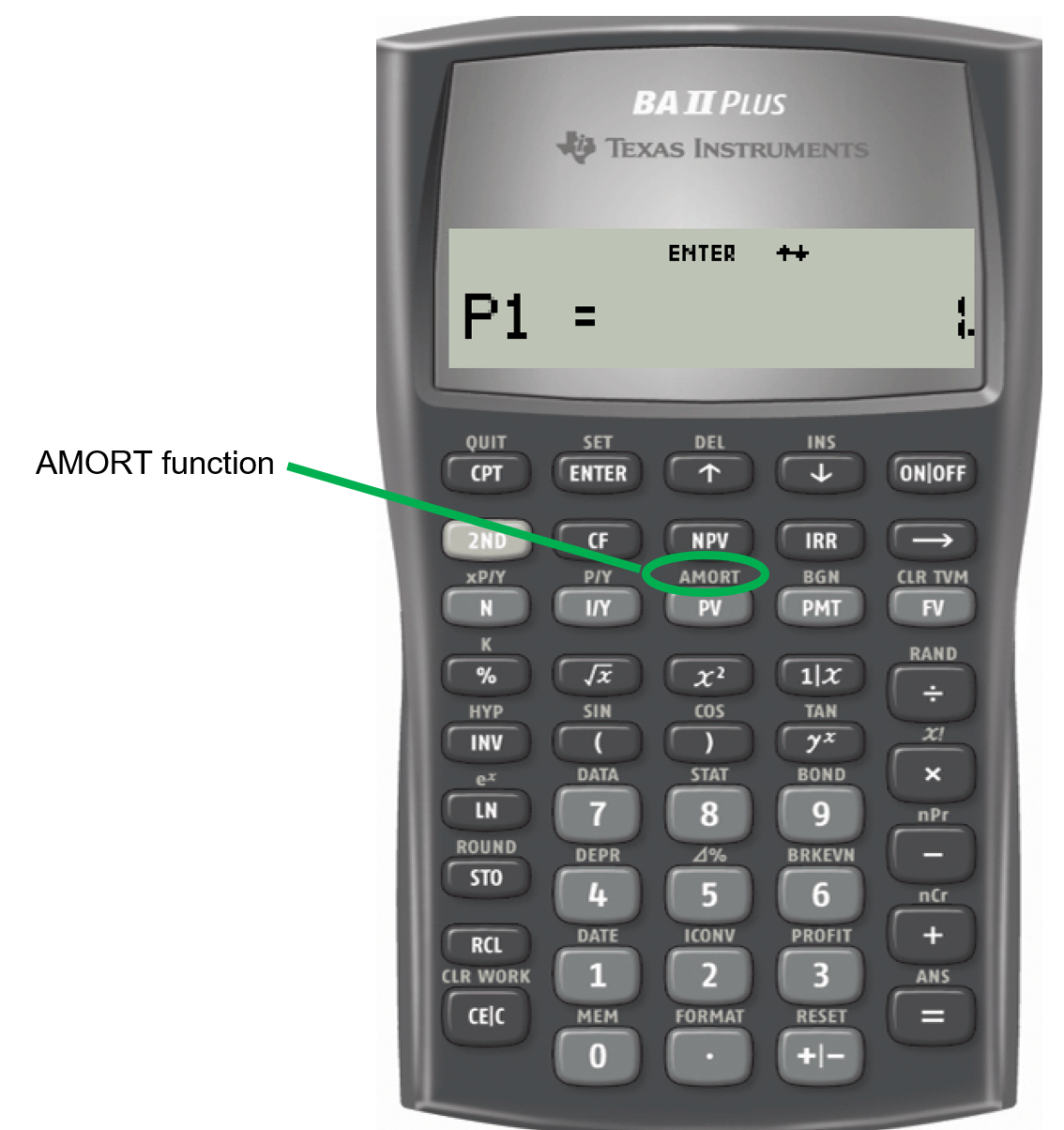
^{\frac{C/Y}{P/Y}}-1=(1+0.02)^{\frac{4}{12}}-1=0.00662271\; \text{per month}")
}=12 \times 2 =24")
![\begin{align} PV_{ORD}&=PMT \left[\frac{1-(1+i_{eq})^{-n}}{i_{eq}}\right]\\ \$10,\!000&=PMT\left[\frac{1-(1+0.00662271)^{-24}}{0.00662271}\right]\\ \$10,\!000&=PMT\left[\frac{0.146509}{0.00662271}\right]\\ \$10,\!000&=PMT (22.122213)\\ PMT&=\frac{\$10,\!000}{22.122213}=\$452.03 \end{align}](https://jin71j2ebb.execute-api.ca-central-1.amazonaws.com/latest/latex?latex=%5Cbegin%7Balign%7D%20%20PV_%7BORD%7D%26%3DPMT%20%5Cleft%5B%5Cfrac%7B1-%281%2Bi_%7Beq%7D%29%5E%7B-n%7D%7D%7Bi_%7Beq%7D%7D%5Cright%5D%5C%5C%20%20%5C%2410%2C%5C%21000%26%3DPMT%5Cleft%5B%5Cfrac%7B1-%281%2B0.00662271%29%5E%7B-24%7D%7D%7B0.00662271%7D%5Cright%5D%5C%5C%20%20%5C%2410%2C%5C%21000%26%3DPMT%5Cleft%5B%5Cfrac%7B0.146509%7D%7B0.00662271%7D%5Cright%5D%5C%5C%20%20%5C%2410%2C%5C%21000%26%3DPMT%20%2822.122213%29%5C%5C%20%20PMT%26%3D%5Cfrac%7B%5C%2410%2C%5C%21000%7D%7B22.122213%7D%3D%5C%24452.03%20%20%5Cend%7Balign%7D&fg=000000&font=TeX&svg=1 "\begin{align} PV_{ORD}&=PMT \left[\frac{1-(1+i_{eq})^{-n}}{i_{eq}}\right]\\ \$10,\!000&=PMT\left[\frac{1-(1+0.00662271)^{-24}}{0.00662271}\right]\\ \$10,\!000&=PMT\left[\frac{0.146509}{0.00662271}\right]\\ \$10,\!000&=PMT (22.122213)\\ PMT&=\frac{\$10,\!000}{22.122213}=\$452.03 \end{align}")
^n\\ &=\$10,\!000(1+0.00662271)^9\\ &=\$10,\!612.08 \end{align}")
![\begin{align} FV_{ORD}&=PMT \left[\frac{(1+i_{eq})^n-1}{i_{eq}}\right]\\ &=\$452.03\left[\frac{(1+0.00662271)^9-1}{0.00662271}\right]\\ &=\$4,\!177.723942 \end{align}](https://jin71j2ebb.execute-api.ca-central-1.amazonaws.com/latest/latex?latex=%5Cbegin%7Balign%7D%20%20FV_%7BORD%7D%26%3DPMT%20%5Cleft%5B%5Cfrac%7B%281%2Bi_%7Beq%7D%29%5En-1%7D%7Bi_%7Beq%7D%7D%5Cright%5D%5C%5C%20%20%26%3D%5C%24452.03%5Cleft%5B%5Cfrac%7B%281%2B0.00662271%29%5E9-1%7D%7B0.00662271%7D%5Cright%5D%5C%5C%20%20%26%3D%5C%244%2C%5C%21177.723942%20%20%5Cend%7Balign%7D&fg=000000&font=TeX&svg=1 "\begin{align} FV_{ORD}&=PMT \left[\frac{(1+i_{eq})^n-1}{i_{eq}}\right]\\ &=\$452.03\left[\frac{(1+0.00662271)^9-1}{0.00662271}\right]\\ &=\$4,\!177.723942 \end{align}")

}=4 \times 5 =20")
![\begin{align} PV_{ORD}&=PMT \left[\frac{1-(1+i)^{-n}}{i}\right]\\ \$50,\!000&=PMT\left[\frac{1-(1+0.0125)^{-20}}{0.0125}\right]\\ \$50,\!000&=PMT\left[\frac{0.219991452}{0.0125}\right]\\ \$50,\!000&=PMT (17.599316)\\ PMT&=\frac{\$50,\!000}{17.599316}=\$2,\!841.02 \end{align}](https://jin71j2ebb.execute-api.ca-central-1.amazonaws.com/latest/latex?latex=%5Cbegin%7Balign%7D%20%20PV_%7BORD%7D%26%3DPMT%20%5Cleft%5B%5Cfrac%7B1-%281%2Bi%29%5E%7B-n%7D%7D%7Bi%7D%5Cright%5D%5C%5C%20%20%5C%2450%2C%5C%21000%26%3DPMT%5Cleft%5B%5Cfrac%7B1-%281%2B0.0125%29%5E%7B-20%7D%7D%7B0.0125%7D%5Cright%5D%5C%5C%20%20%5C%2450%2C%5C%21000%26%3DPMT%5Cleft%5B%5Cfrac%7B0.219991452%7D%7B0.0125%7D%5Cright%5D%5C%5C%20%20%5C%2450%2C%5C%21000%26%3DPMT%20%2817.599316%29%5C%5C%20%20PMT%26%3D%5Cfrac%7B%5C%2450%2C%5C%21000%7D%7B17.599316%7D%3D%5C%242%2C%5C%21841.02%20%20%5Cend%7Balign%7D&fg=000000&font=TeX&svg=1 "\begin{align} PV_{ORD}&=PMT \left[\frac{1-(1+i)^{-n}}{i}\right]\\ \$50,\!000&=PMT\left[\frac{1-(1+0.0125)^{-20}}{0.0125}\right]\\ \$50,\!000&=PMT\left[\frac{0.219991452}{0.0125}\right]\\ \$50,\!000&=PMT (17.599316)\\ PMT&=\frac{\$50,\!000}{17.599316}=\$2,\!841.02 \end{align}")
^n\\ &=\$50,\!000(1+0.0125)^4\\ &=\$52,\!547.26685 \end{align}")
![\begin{align} FV_{ORD}&=PMT \left[\frac{(1+i)^n-1}{i_{eq}}\right]\\ &=\$2,\!841.02\left[\frac{(1+0.0125)^4-1}{0.0125}\right]\\ &=\$11,\!578.93769 \end{align}](https://jin71j2ebb.execute-api.ca-central-1.amazonaws.com/latest/latex?latex=%5Cbegin%7Balign%7D%20%20FV_%7BORD%7D%26%3DPMT%20%5Cleft%5B%5Cfrac%7B%281%2Bi%29%5En-1%7D%7Bi_%7Beq%7D%7D%5Cright%5D%5C%5C%20%20%26%3D%5C%242%2C%5C%21841.02%5Cleft%5B%5Cfrac%7B%281%2B0.0125%29%5E4-1%7D%7B0.0125%7D%5Cright%5D%5C%5C%20%20%26%3D%5C%2411%2C%5C%21578.93769%20%20%5Cend%7Balign%7D&fg=000000&font=TeX&svg=1 "\begin{align} FV_{ORD}&=PMT \left[\frac{(1+i)^n-1}{i_{eq}}\right]\\ &=\$2,\!841.02\left[\frac{(1+0.0125)^4-1}{0.0125}\right]\\ &=\$11,\!578.93769 \end{align}")


^n\\ &=\$10,\!000(1+0.00662271)^6\\ &=\$10,\!404.00 \end{align}")
![\begin{align} FV_{ORD}&=PMT \left[\frac{(1+i_{eq})^n-1}{i_{eq}}\right]\\ &=\$452.03\left[\frac{(1+0.00662271)^6-1}{0.00662271}\right]\\ &=\$2,\!757.483452 \end{align}](https://jin71j2ebb.execute-api.ca-central-1.amazonaws.com/latest/latex?latex=%5Cbegin%7Balign%7D%20%20FV_%7BORD%7D%26%3DPMT%20%5Cleft%5B%5Cfrac%7B%281%2Bi_%7Beq%7D%29%5En-1%7D%7Bi_%7Beq%7D%7D%5Cright%5D%5C%5C%20%26%3D%5C%24452.03%5Cleft%5B%5Cfrac%7B%281%2B0.00662271%29%5E6-1%7D%7B0.00662271%7D%5Cright%5D%5C%5C%20%26%3D%5C%242%2C%5C%21757.483452%20%20%5Cend%7Balign%7D&fg=000000&font=TeX&svg=1 "\begin{align} FV_{ORD}&=PMT \left[\frac{(1+i_{eq})^n-1}{i_{eq}}\right]\\ &=\$452.03\left[\frac{(1+0.00662271)^6-1}{0.00662271}\right]\\ &=\$2,\!757.483452 \end{align}")
^n\\ &=\$10,\!000(1+0.00662271)^{18}\\ &=\$11,\!261.62428 \end{align}")
![\begin{align} FV_{ORD}&=PMT \left[\frac{(1+i_{eq})^n-1}{i_{eq}}\right]\\ &=\$452.03\left[\frac{(1+0.00662271)^{18}-1}{0.00662271}\right]\\ &=\$8,\!611.1580 \end{align}](https://jin71j2ebb.execute-api.ca-central-1.amazonaws.com/latest/latex?latex=%5Cbegin%7Balign%7D%20%20FV_%7BORD%7D%26%3DPMT%20%5Cleft%5B%5Cfrac%7B%281%2Bi_%7Beq%7D%29%5En-1%7D%7Bi_%7Beq%7D%7D%5Cright%5D%5C%5C%20%20%26%3D%5C%24452.03%5Cleft%5B%5Cfrac%7B%281%2B0.00662271%29%5E%7B18%7D-1%7D%7B0.00662271%7D%5Cright%5D%5C%5C%20%20%26%3D%5C%248%2C%5C%21611.1580%20%20%5Cend%7Balign%7D&fg=000000&font=TeX&svg=1 "\begin{align} FV_{ORD}&=PMT \left[\frac{(1+i_{eq})^n-1}{i_{eq}}\right]\\ &=\$452.03\left[\frac{(1+0.00662271)^{18}-1}{0.00662271}\right]\\ &=\$8,\!611.1580 \end{align}")
^n\\ &=\$50,\!000(1+0.0125)^8\\ &=\$55,\!224.30506 \end{align}")
![\begin{align} FV_{ORD}&=PMT \left[\frac{(1+i)^n-1}{i}\right]\\ &=\$2,\!841.02\left[\frac{(1+0.0125)^8-1}{0.0125}\right]\\ &=\$23,\!747.76825 \end{align}](https://jin71j2ebb.execute-api.ca-central-1.amazonaws.com/latest/latex?latex=%5Cbegin%7Balign%7D%20%20FV_%7BORD%7D%26%3DPMT%20%5Cleft%5B%5Cfrac%7B%281%2Bi%29%5En-1%7D%7Bi%7D%5Cright%5D%5C%5C%20%20%26%3D%5C%242%2C%5C%21841.02%5Cleft%5B%5Cfrac%7B%281%2B0.0125%29%5E8-1%7D%7B0.0125%7D%5Cright%5D%5C%5C%20%20%26%3D%5C%2423%2C%5C%21747.76825%20%20%5Cend%7Balign%7D&fg=000000&font=TeX&svg=1 "\begin{align} FV_{ORD}&=PMT \left[\frac{(1+i)^n-1}{i}\right]\\ &=\$2,\!841.02\left[\frac{(1+0.0125)^8-1}{0.0125}\right]\\ &=\$23,\!747.76825 \end{align}")
^n\\ &=\$50,\!000(1+0.0125)^{12}\\ &=\$58,\!037.72589 \end{align}")
![\begin{align} FV_{ORD}&=PMT \left[\frac{(1+i)^n-1}{i_{eq}}\right]\\ &=\$2,\!841.02\left[\frac{(1+0.0125)^{12}-1}{0.0125}\right]\\ &=\$36,\!536.544 \end{align}](https://jin71j2ebb.execute-api.ca-central-1.amazonaws.com/latest/latex?latex=%5Cbegin%7Balign%7D%20%20FV_%7BORD%7D%26%3DPMT%20%5Cleft%5B%5Cfrac%7B%281%2Bi%29%5En-1%7D%7Bi_%7Beq%7D%7D%5Cright%5D%5C%5C%20%20%26%3D%5C%242%2C%5C%21841.02%5Cleft%5B%5Cfrac%7B%281%2B0.0125%29%5E%7B12%7D-1%7D%7B0.0125%7D%5Cright%5D%5C%5C%20%20%26%3D%5C%2436%2C%5C%21536.544%20%20%5Cend%7Balign%7D&fg=000000&font=TeX&svg=1 "\begin{align} FV_{ORD}&=PMT \left[\frac{(1+i)^n-1}{i_{eq}}\right]\\ &=\$2,\!841.02\left[\frac{(1+0.0125)^{12}-1}{0.0125}\right]\\ &=\$36,\!536.544 \end{align}")
^n\\ &=\$10,\!000(1+0.00662271)^{23}\\ &=\$11,\!639.50884 \end{align}")
![\begin{align} FV_{ORD}&=PMT \left[\frac{(1+i_{eq})^n-1}{i_{eq}}\right]\\ &=\$452.03\left[\frac{(1+0.00662271)^{23}-1}{0.00662271}\right]\\ &=\$11,\!190.39157 \end{align}](https://jin71j2ebb.execute-api.ca-central-1.amazonaws.com/latest/latex?latex=%5Cbegin%7Balign%7D%20%20FV_%7BORD%7D%26%3DPMT%20%5Cleft%5B%5Cfrac%7B%281%2Bi_%7Beq%7D%29%5En-1%7D%7Bi_%7Beq%7D%7D%5Cright%5D%5C%5C%20%20%26%3D%5C%24452.03%5Cleft%5B%5Cfrac%7B%281%2B0.00662271%29%5E%7B23%7D-1%7D%7B0.00662271%7D%5Cright%5D%5C%5C%20%20%26%3D%5C%2411%2C%5C%21190.39157%20%20%5Cend%7Balign%7D&fg=000000&font=TeX&svg=1 "\begin{align} FV_{ORD}&=PMT \left[\frac{(1+i_{eq})^n-1}{i_{eq}}\right]\\ &=\$452.03\left[\frac{(1+0.00662271)^{23}-1}{0.00662271}\right]\\ &=\$11,\!190.39157 \end{align}")
^n\\ &=\$50,\!000(1+0.0125)^{19}\\ &=\$63,\!310.48058 \end{align}")
![\begin{align} FV_{ORD}&=PMT \left[\frac{(1+i)^n-1}{i_{eq}}\right]\\ &=\$2,\!841.02\left[\frac{(1+0.0125)^{19}-1}{0.0125}\right]\\ &=\$60,\!504.54645 \end{align}](https://jin71j2ebb.execute-api.ca-central-1.amazonaws.com/latest/latex?latex=%5Cbegin%7Balign%7D%20%20FV_%7BORD%7D%26%3DPMT%20%5Cleft%5B%5Cfrac%7B%281%2Bi%29%5En-1%7D%7Bi_%7Beq%7D%7D%5Cright%5D%5C%5C%20%20%26%3D%5C%242%2C%5C%21841.02%5Cleft%5B%5Cfrac%7B%281%2B0.0125%29%5E%7B19%7D-1%7D%7B0.0125%7D%5Cright%5D%5C%5C%20%20%26%3D%5C%2460%2C%5C%21504.54645%20%20%5Cend%7Balign%7D&fg=000000&font=TeX&svg=1 "\begin{align} FV_{ORD}&=PMT \left[\frac{(1+i)^n-1}{i_{eq}}\right]\\ &=\$2,\!841.02\left[\frac{(1+0.0125)^{19}-1}{0.0125}\right]\\ &=\$60,\!504.54645 \end{align}")
^n\\ &=\$10,\!000(1+0.00662271)^{12}\\ &=\$10,\!824.32166 \end{align}")
![\begin{align} FV_{ORD}&=PMT \left[\frac{(1+i_{eq})^n-1}{i_{eq}}\right]\\ &=\$452.03\left[\frac{(1+0.00662271)^{12}-1}{0.00662271}\right]\\ &=\$5,\!626.369243 \end{align}](https://jin71j2ebb.execute-api.ca-central-1.amazonaws.com/latest/latex?latex=%5Cbegin%7Balign%7D%20%20FV_%7BORD%7D%26%3DPMT%20%5Cleft%5B%5Cfrac%7B%281%2Bi_%7Beq%7D%29%5En-1%7D%7Bi_%7Beq%7D%7D%5Cright%5D%5C%5C%20%20%26%3D%5C%24452.03%5Cleft%5B%5Cfrac%7B%281%2B0.00662271%29%5E%7B12%7D-1%7D%7B0.00662271%7D%5Cright%5D%5C%5C%20%20%26%3D%5C%245%2C%5C%21626.369243%20%20%5Cend%7Balign%7D&fg=000000&font=TeX&svg=1 "\begin{align} FV_{ORD}&=PMT \left[\frac{(1+i_{eq})^n-1}{i_{eq}}\right]\\ &=\$452.03\left[\frac{(1+0.00662271)^{12}-1}{0.00662271}\right]\\ &=\$5,\!626.369243 \end{align}")
^n\\ &=\$10,\!000(1+0.00662271)^{24}\\ &=\$11,\!716.59393 \end{align}")
![\begin{align} FV_{ORD}&=PMT \left[\frac{(1+i_{eq})^n-1}{i_{eq}}\right]\\ &=\$452.03\left[\frac{(1+0.00662271)^{24}-1}{0.00662271}\right]\\ &=\$11,\!716.53229 \end{align}](https://jin71j2ebb.execute-api.ca-central-1.amazonaws.com/latest/latex?latex=%5Cbegin%7Balign%7D%20%20FV_%7BORD%7D%26%3DPMT%20%5Cleft%5B%5Cfrac%7B%281%2Bi_%7Beq%7D%29%5En-1%7D%7Bi_%7Beq%7D%7D%5Cright%5D%5C%5C%20%20%26%3D%5C%24452.03%5Cleft%5B%5Cfrac%7B%281%2B0.00662271%29%5E%7B24%7D-1%7D%7B0.00662271%7D%5Cright%5D%5C%5C%20%20%26%3D%5C%2411%2C%5C%21716.53229%20%20%5Cend%7Balign%7D&fg=000000&font=TeX&svg=1 "\begin{align} FV_{ORD}&=PMT \left[\frac{(1+i_{eq})^n-1}{i_{eq}}\right]\\ &=\$452.03\left[\frac{(1+0.00662271)^{24}-1}{0.00662271}\right]\\ &=\$11,\!716.53229 \end{align}")
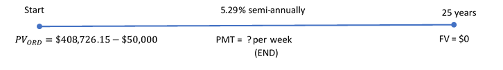
 find the equivalent rate
^{\frac{C/Y}{P/Y}}-1=(1+0.02645)^{\frac{2}{52}}-1=0.001004591\; \text{per week}")
=52 \times 25 =1,\!300")
![\begin{align} PV_{ORD}&=PMT \left[\frac{1-(1+i_{eq})^{-n}}{i_{eq}}\right]\\ $358,\!726.16&=PMT\left[\frac{1-(1+0.001004591)^{-1300}}{0.001004591}\right]\\ $358,\!726.16&=PMT \frac{0.728912263}{0.001004591}\\ $358,\!726.16&=PMT(725.5811199)\\ PMT&=\$494.40 \end{align}](https://jin71j2ebb.execute-api.ca-central-1.amazonaws.com/latest/latex?latex=%5Cbegin%7Balign%7D%20%20PV_%7BORD%7D%26%3DPMT%20%5Cleft%5B%5Cfrac%7B1-%281%2Bi_%7Beq%7D%29%5E%7B-n%7D%7D%7Bi_%7Beq%7D%7D%5Cright%5D%5C%5C%20%20%24358%2C%5C%21726.16%26%3DPMT%5Cleft%5B%5Cfrac%7B1-%281%2B0.001004591%29%5E%7B-1300%7D%7D%7B0.001004591%7D%5Cright%5D%5C%5C%20%20%24358%2C%5C%21726.16%26%3DPMT%20%5Cfrac%7B0.728912263%7D%7B0.001004591%7D%5C%5C%20%20%24358%2C%5C%21726.16%26%3DPMT%28725.5811199%29%5C%5C%20%20PMT%26%3D%5C%24494.40%20%20%5Cend%7Balign%7D&fg=000000&font=TeX&svg=1 "\begin{align} PV_{ORD}&=PMT \left[\frac{1-(1+i_{eq})^{-n}}{i_{eq}}\right]\\ $358,\!726.16&=PMT\left[\frac{1-(1+0.001004591)^{-1300}}{0.001004591}\right]\\ $358,\!726.16&=PMT \frac{0.728912263}{0.001004591}\\ $358,\!726.16&=PMT(725.5811199)\\ PMT&=\$494.40 \end{align}")

^{\frac{C/Y}{P/Y}}-1=(1+0.0245)^{\frac{2}{12}}-1=0.004042263\; \text{per month}")
=12 \times 20 =240")
![\begin{align} PV_{ORD}&=PMT \left[\frac{1-(1+i_{eq})^{-n}}{i_{eq}}\right]\\ $350,\!100&=PMT\left[\frac{1-(1+0.004042263)^{-240}}{0.004042263}\right]\\ $350,\!100&=PMT \frac{0.620229289}{0.004042263}\\ $350,\!100&=PMT(153.4361543)\\ PMT&=\$2,\!281.73 \end{align}](https://jin71j2ebb.execute-api.ca-central-1.amazonaws.com/latest/latex?latex=%5Cbegin%7Balign%7D%20%20PV_%7BORD%7D%26%3DPMT%20%5Cleft%5B%5Cfrac%7B1-%281%2Bi_%7Beq%7D%29%5E%7B-n%7D%7D%7Bi_%7Beq%7D%7D%5Cright%5D%5C%5C%20%20%24350%2C%5C%21100%26%3DPMT%5Cleft%5B%5Cfrac%7B1-%281%2B0.004042263%29%5E%7B-240%7D%7D%7B0.004042263%7D%5Cright%5D%5C%5C%20%20%24350%2C%5C%21100%26%3DPMT%20%5Cfrac%7B0.620229289%7D%7B0.004042263%7D%5C%5C%20%20%24350%2C%5C%21100%26%3DPMT%28153.4361543%29%5C%5C%20%20PMT%26%3D%5C%242%2C%5C%21281.73%20%20%5Cend%7Balign%7D&fg=000000&font=TeX&svg=1 "\begin{align} PV_{ORD}&=PMT \left[\frac{1-(1+i_{eq})^{-n}}{i_{eq}}\right]\\ $350,\!100&=PMT\left[\frac{1-(1+0.004042263)^{-240}}{0.004042263}\right]\\ $350,\!100&=PMT \frac{0.620229289}{0.004042263}\\ $350,\!100&=PMT(153.4361543)\\ PMT&=\$2,\!281.73 \end{align}")

^n\\ &=\$350,\!100(1+0.004042263)^{36}\\ &=\$404,\!821.7991 \end{align}")
![\begin{align} FV_{ORD}&=PMT \left[\frac{(1+i_{eq})^n-1}{i_{eq}}\right]\\ &=\$2,\!281.73\left[\frac{(1+0.004042263)^{36}-1}{0.004042263}\right]\\ &=\$88,\!228.30644 \end{align}](https://jin71j2ebb.execute-api.ca-central-1.amazonaws.com/latest/latex?latex=%5Cbegin%7Balign%7D%20%20FV_%7BORD%7D%26%3DPMT%20%5Cleft%5B%5Cfrac%7B%281%2Bi_%7Beq%7D%29%5En-1%7D%7Bi_%7Beq%7D%7D%5Cright%5D%5C%5C%20%20%26%3D%5C%242%2C%5C%21281.73%5Cleft%5B%5Cfrac%7B%281%2B0.004042263%29%5E%7B36%7D-1%7D%7B0.004042263%7D%5Cright%5D%5C%5C%20%20%26%3D%5C%2488%2C%5C%21228.30644%20%20%5Cend%7Balign%7D&fg=000000&font=TeX&svg=1 "\begin{align} FV_{ORD}&=PMT \left[\frac{(1+i_{eq})^n-1}{i_{eq}}\right]\\ &=\$2,\!281.73\left[\frac{(1+0.004042263)^{36}-1}{0.004042263}\right]\\ &=\$88,\!228.30644 \end{align}")

^{\frac{C/Y}{P/Y}}-1=(1+0.02925)^{\frac{2}{12}}-1=0.004816626\; \text{per month}")
=12 \times 17 =204\;\text{payments}")
![\begin{align} PV_{ORD}&=PMT \left[\frac{1-(1+i_{eq})^{-n}}{i_{eq}}\right]\\ $316,\!593.49&=PMT\left[\frac{1-(1+0.004816626)^{-204}}{0.004816626}\right]\\ $316,\!593.49&=PMT \frac{0.624776296}{0.004816626}\\ $316,\!593.49&=PMT(129.7124369)\\ PMT&=\$2,\!440.73 \end{align}](https://jin71j2ebb.execute-api.ca-central-1.amazonaws.com/latest/latex?latex=%5Cbegin%7Balign%7D%20%20PV_%7BORD%7D%26%3DPMT%20%5Cleft%5B%5Cfrac%7B1-%281%2Bi_%7Beq%7D%29%5E%7B-n%7D%7D%7Bi_%7Beq%7D%7D%5Cright%5D%5C%5C%20%20%24316%2C%5C%21593.49%26%3DPMT%5Cleft%5B%5Cfrac%7B1-%281%2B0.004816626%29%5E%7B-204%7D%7D%7B0.004816626%7D%5Cright%5D%5C%5C%20%20%24316%2C%5C%21593.49%26%3DPMT%20%5Cfrac%7B0.624776296%7D%7B0.004816626%7D%5C%5C%20%20%24316%2C%5C%21593.49%26%3DPMT%28129.7124369%29%5C%5C%20%20PMT%26%3D%5C%242%2C%5C%21440.73%20%20%5Cend%7Balign%7D&fg=000000&font=TeX&svg=1 "\begin{align} PV_{ORD}&=PMT \left[\frac{1-(1+i_{eq})^{-n}}{i_{eq}}\right]\\ $316,\!593.49&=PMT\left[\frac{1-(1+0.004816626)^{-204}}{0.004816626}\right]\\ $316,\!593.49&=PMT \frac{0.624776296}{0.004816626}\\ $316,\!593.49&=PMT(129.7124369)\\ PMT&=\$2,\!440.73 \end{align}")


 = interest portion of an ordinary single annuity payment or a series of annuity payments


 ;
;  ;
; 
}\\ &=\$34,\!285.71 \end{align}")
 ;
;  ;
; 

}\\ &=5\;\text{months} \end{align}")
 ;
;  ;
; 

}\\ &=0.04 \;\text{or}\;4\% \end{align}")
 ;
;  ;
; 


\left(\frac{197}{365}\right)\\ & = \$1,\!619.18 \end{align}")
 ;
;  ;
; 

}\\ &=146.995454\; \text{days}\;\rightarrow 147\; \text{days} \end{align}")
 ;
;  ;
; 


 ;
;  ;
; 


}\\ & = 0.078004 \;\text{or}\; 7.8004\% \end{align}")

 ;
; 
 ;
; 

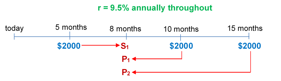

 .
.\\ & = \$2,\!000 \times \left(1 + 0.095 \times \frac{3}{12}\right)\\ & = \$2,\!000 \times 1.02375\\ &= \$2,\!047.50 \end{align}")

 .
.

 .
.


 ;
; 

 ;
; 
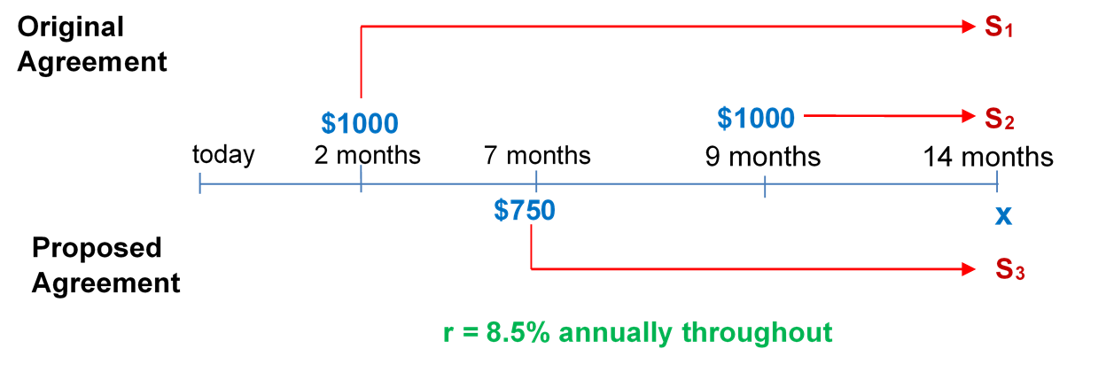

\\ & = \$1,\!000 \times (1 + 0.085 \times 1)\\ &= \$1,\!085 \end{align}")

 .
.\\ & = \$1,\!000 \times \left(1 + 0.085 \times \frac{5}{12}\right)\\ &= \$1,\!035.42 \end{align}")
 .
.\\ & = \$775 \times \left(1 + 0.085 \times \frac{7}{12}\right)\\ &= \$813.43 \end{align}")


\left(\frac{2}{365}\right)\\ &= \$31.356164 \end{align}")

\left(\frac{10}{365}\right)\\ &= \$286.232876 \end{align}")

\left(\frac{10}{365}\right)\\ &= \$32.876712 \end{align}")

\left(\frac{8}{365}\right)\\ &= \$171.452054 \end{align}")
\left(\frac{3}{365}\right)\\ &= \$85.869863 \end{align}")

\left(\frac{3}{365}\right)\\ &= \$23.013698 \end{align}")
\left(\frac{8}{365}\right)\\ &= \$228.986301 \end{align}")

\left(\frac{8}{365}\right)\\ &= \$8.767123 \end{align}")

 ;
;  ;
; 

\\ & = \$25,\!500 \times \left(1 + 0.0055 \times \frac{80}{365}\right)\\ &= \$25,\!530.74 \end{align}")
 ;
; 
 ;
; 
 ;
;  ;
; and
and 
\\ &= \$50,\!098.63 \end{align}")
\\ &= \$50,\!036.99 \end{align}")
 – (\text {S of}\; 90-\text{day GIC})")
 \end{align}")
}\\ & = 0.004995\;\text{or}\;0.4995\% \end{align}")
 ;
;  ;
; 

") ;
; 


") ;
; 


 ;
; 
\\ &= 3+25\\ &= 28 \;\text{days or}\; 28/365 \end{align}")

 ;
;  ;
; 


 ;
; 


 ;
; 


 \end{align}")
 \times (\text{Compounds Per Year})\\ &= 2.0875\% \times 4\\ &=8.35\%\; \text{compounded quarterly} \end{align}")

 \times (\text{Compounds Per Year})\\ &= 1.8\% \times 4\\ &=7.2\%\; \text{compounded quarterly} \end{align}")
 ;
;  ;
;  ;
; 
}}{\text{Compound per year (C/Y)}}=\frac{6\%}{12}=0.5\%")
 \times C/Y= \left(4\frac{3}{12}\right) \times 12=4.25 \times 12=51")
^{51}\\ &= \$53,\!000(1 + 0.005)^{51}\\ &= \$53,\!000(1.005)^{51}\\ &= \$68,\!351.02 \end{align}")
 .
.}}{\text{Compounds per Year (C/Y)}}=\frac{4.1\%}{1}=4.1\%")
 \times C/Y=4 \times 1=4")
^n\\ &= \$24,\!500 (1 + 0.041)^4\\ &= \$24,\!500(1.041)^4\\ &= \$28,\!771.93049\; \text{(This becomes PV for the next calculation in Step 2.)} \end{align}")
 .
.}}{\text{Compounds per Year (C/Y)}}=\frac{5.15\%}{4}=1.2875\%")
 \times C/Y= \left(1\frac{9}{12}\right) \times 4=1.75 \times 4=7")
^n\\ &= \$28,\!771.93049 (1.012875)^7\\ &= \$31,\!467.33516\; \text{(This becomes PV for the next calculation in Step 3.)} \end{align}")
 .
.}}{\text{Compounds per Year (C/Y)}}=\frac{5.35\%}{12}=0.4458\overline{3}\%")
 \times C/Y= \left(1\frac{3}{12}\right) \times 12=1.25 \times 12=15")
^n\\ &= \$31,\!467.33516 (1.004458\overline{3})^{15}\\ &= \$33,\!638.67 \end{align}")
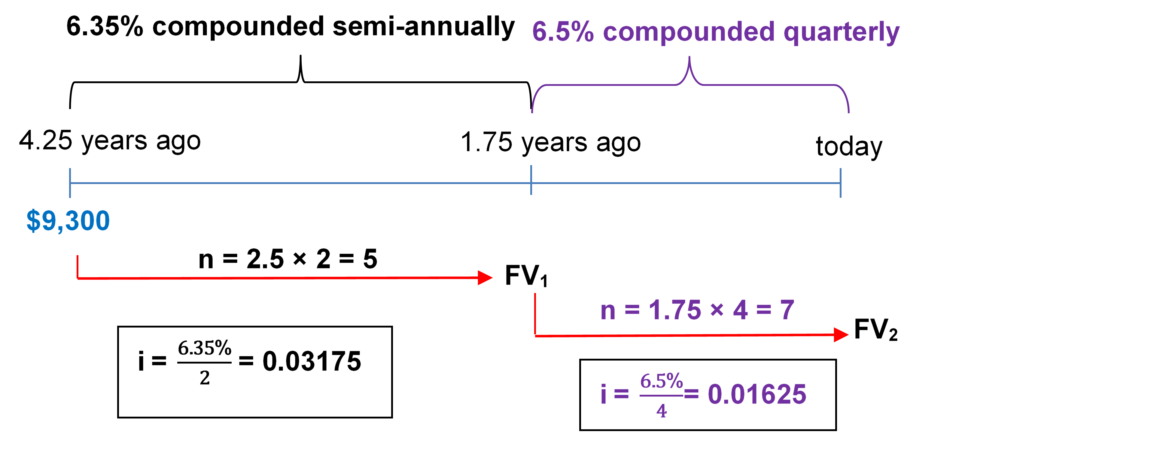
}}{\text{Compounds per Year (C/Y)}}=\frac{6.35\%}{2}=3.175\%")
 \times C/Y=2.5 \times 2=5")
^n\\ &= \$9,\!300(1. 03175)^5\\ &= \$10,\!873.14892\; \text{(This becomes PV for the next calculation in Step 2.)} \end{align}")
}}{\text{Compounds per Year (C/Y)}}=\frac{6.5\%}{4}=1.625\%")
 \times C/Y=1.75 \times 4=7")
^n\\ &= \$10,\!873.14892(1. 001625)^7\\ &= \$12,\!171.92\; \text{(Round at this step.)} \end{align}")
 ;
;  ;
;  ;
; .
.}}{\text{Compounds per Year (C/Y)}}=\frac{6.55\%}{4}=1.6375\%")
 \times C/Y=\frac{21}{12} \times 4=7")
^n}\\ &=\frac{\$37,\!000}{(1.016375)^7}\\ &=\$33,\!023.56 \end{align}")
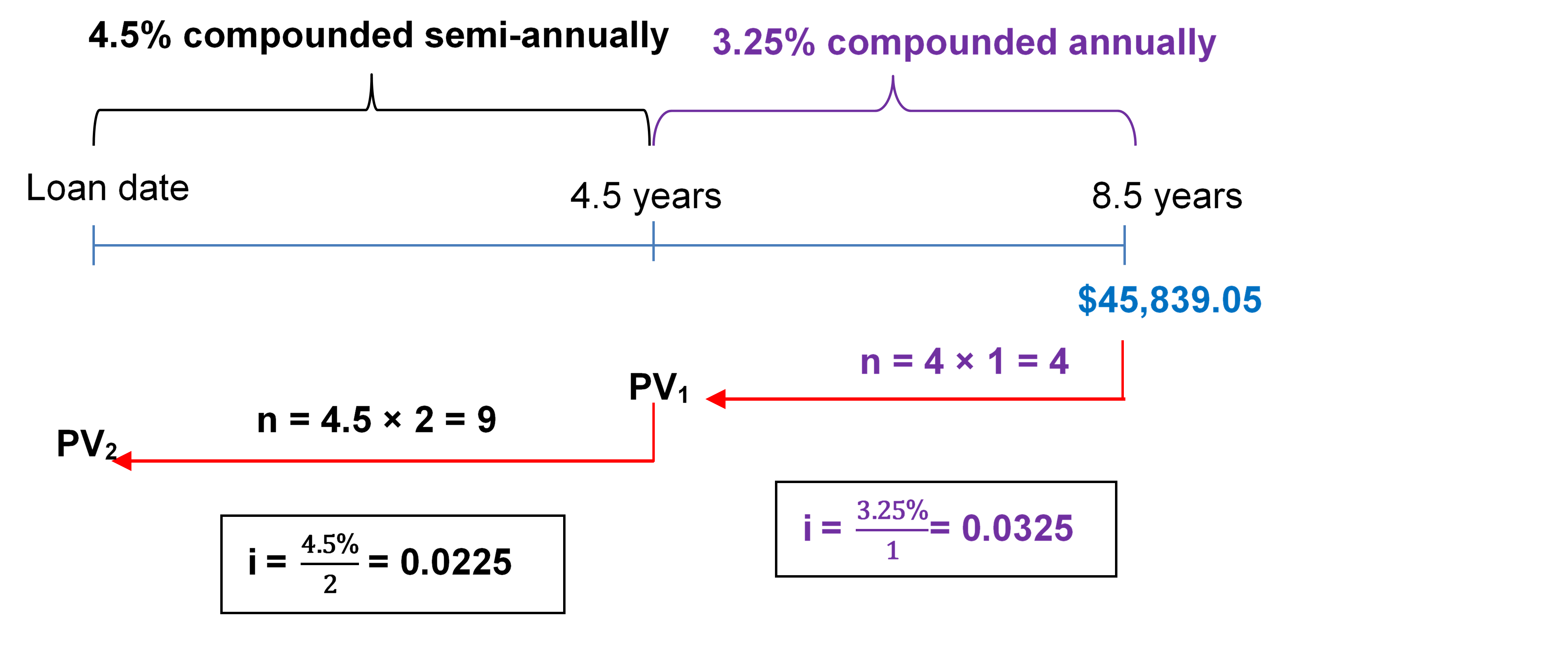
 .
.}}{\text{Compounds per Year (C/Y)}}=\frac{3.25\%}{1}=3.25\%")
} \times C/Y=4 \times 1=4")
^n}\\ &=\frac{\$45,\!839.05}{(1.0325)^4}\\ &=\$40,\!334.37829\;\text{(This becomes FV for the next calculation in Step 2.)} \end{align}")
 .
.}}{\text{Compounds per Year (C/Y)}}=\frac{4.5\%}{2}=2.25\%")
 \times C/Y=4.5 \times 2=9")
^n}\\ &=\frac{\$40,\!334.37829}{(1.0225)^9}\\ &=\$33,\!014.56\;\text{(Round at this step.)} \end{align}")
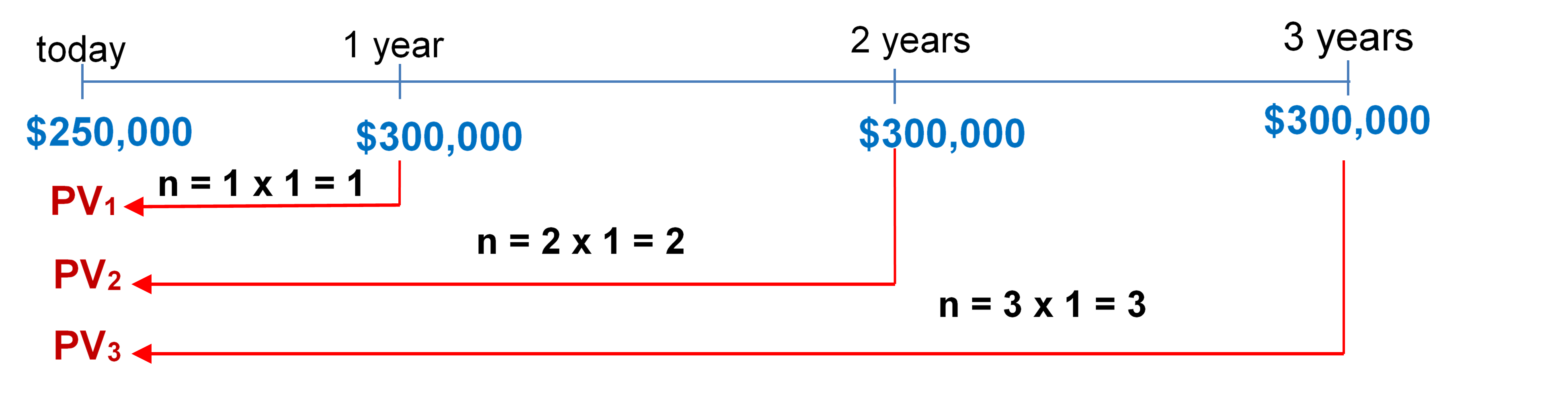

}}{\text{Compounds per Year (C/Y)}}=\frac{9\%}{1}=9\%")
 \times C/Y")


^n}\\ &=\frac{\$300,\!000}{(1.09)^1}\\ &=\$275,\!229.3578 \end{align}")
^n}\\ &=\frac{\$300,\!000}{(1.09)^2}\\ &=\$252,\!503.998 \end{align}")
^n}\\ &=\frac{\$300,\!000}{(1.09)^3}\\ &=\$231,\!655.044 \end{align}")

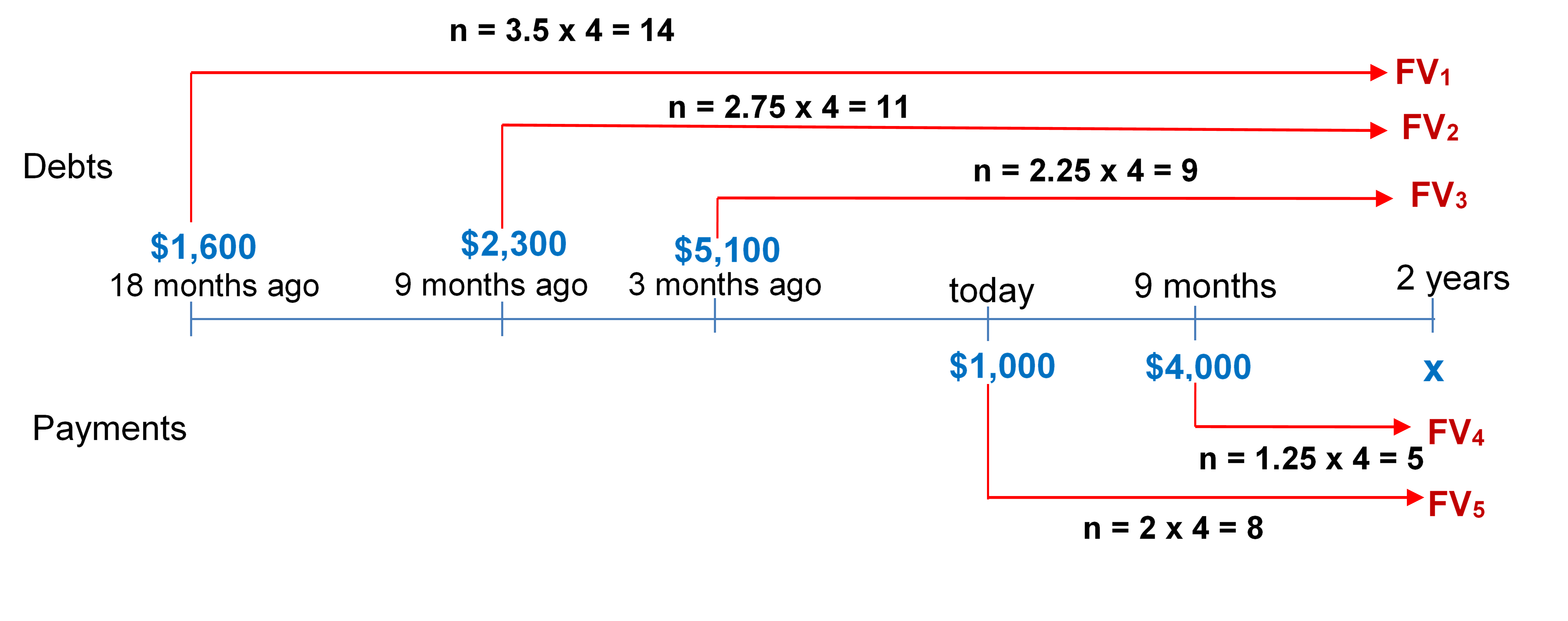

}}{\text{Compounds per Year (C/Y)}}=\frac{16.5\%}{4}=4.125\%")


^{14} = \$2,\!817.670366")
^{11} = \$3,\!587.839398")
^{9} = \$7,\!337.790461")
^{5} = \$4,\!895.928462")
^{8} = \$1,\!381.783859")

 \times C/Y=5 \times 4=20")
^n\\ & = \$5,\!000(1.02)^{20}\\ &=\$7,\!429.74\;\text{(Due in 1 year from today.)} \end{align}")
 \times C/Y=4 \times 12=48")
^n\\ & = \$2,\!500(1.005)^{48}\\ &=\$3,\!176.22\; \text{(Due in 2 year from today.)} \end{align}")
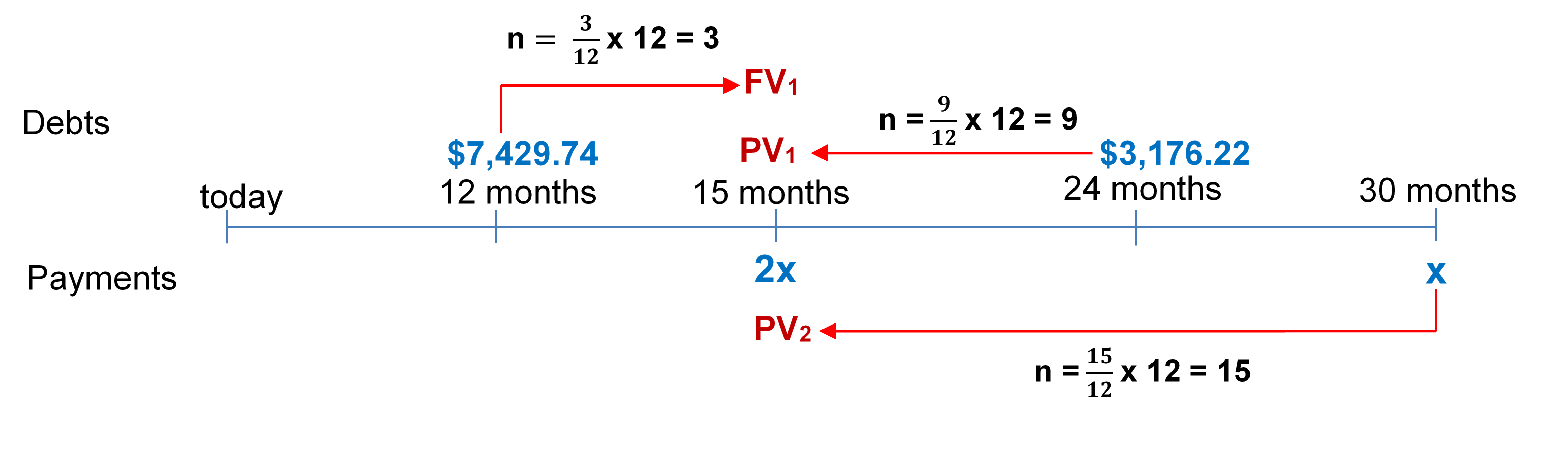

^3 +\frac{3,\!176.22}{(1.005225)^9} &= 2x + \frac{x}{(1.005225)^{15}}\\ 7,\!546.810744 + 3,\!030.686729 &= 2x + 0.924806x\\ \$10,\!577.49747 &= 2.924806x\\ x &= \$3,\!616.48\; \text{(second payment)}\\\\ 2x = 2(\$3,\!616.48) &= $7,\!232.96\; \text{(first payment)} \end{align}")
 ;
;  ;
;  \times C/Y=\frac{5}{12} \times 12=5")
^n\\ \$6,\!948.48 &= \$6,\!450(1 + i)^5\\ 1.077283 &= (1+i)^5\\ 1.077283^{\frac{1}{5}} &= (1+i)\\ 1.014999 &= 1 + i\\ i& = 0.014999 \end{align}")
} \end{align}")
 ;
; 
 \times C/Y=5 \times 12=60")
^n\\ \$20,\!000&= \$10,\!000(1 + i)^{60}\\ 2&= (1+i)^{60}\\ 2^{\frac{1}{60}}& = (1+i)\\ 1.011619 &= 1 + i\\ i& = 0.011619 \end{align}")

} \times C/Y=1 \times 2=2")


^2} = \$28,\!718.86385\end{align}")
^2} = \$27,\!401.82101\end{align}")
^2} = \$26,\!247.63224\end{align}")
^2} = \$25,\!203.68913\end{align}")
^2} = \$24,\!225\end{align}")
} \times C/Y= 5\times 4=20")
^n\\ \$30,\!320.12& = \$24,\!225(1+i)^{20}\\ 1.251604 &= (1+i)^{20}\\ 1.251604^{\frac{1}{20}}&= 1+i\\ 1.011284 &= 1+i\\ i &= 0.011284 \end{align}")

 ;
;  ;
; 

^{\frac{C/Y_{\text{Old}}}{C/Y _{\text{New}}}}-1\\ &=(1+0.02203890)^{\frac{12}{1}}-1\\ &=(1.02203890)^{12}-1\\ &=1.299-1\\ &=0.299 \end{align}")
 ;
; 
^{\frac{C/Y_{\text{Old}}}{C/Y _{\text{New}}}}-1\\ &=(1+0.00691\overline{6})^{\frac{12}{1}}-1\\ &=(1.00691\overline{6})^{12}-1\\ &=1.086231-1\\ &=0.086231 \end{align}")
 ;
;  ;
; 
^{\frac{C/Y_{\text{Old}}}{C/Y _{\text{New}}}}-1\\ &=(1+0.02085)^{\frac{4}{1}}-1\\ &=(1.02085)^{4}-1\\ &=1.086044-1\\ &=0.086045 \end{align}")
 ;
;  ;
; 
^{\frac{C/Y_{\text{Old}}}{C/Y _{\text{New}}}}-1\\ &=(1+0.04225)^{\frac{2}{1}}-1 \\ &=(1.04225)^{2}-1\\ &=1.086285-1\\ &=0.086285 \end{align}")
 ;
;  ;
; 
^{\frac{C/Y_{\text{Old}}}{C/Y _{\text{New}}}}-1\\ &=(1+0.00052238)^{\frac{365}{1}}-1\\ &=(1.00052238)^{365}-1\\ &=1.209999-1\\ &=0.21 \end{align}")
 ;
; ^{\frac{C/Y_{\text{Old}}}{C/Y _{\text{New}}}}-1\\ 0.22&=(1+i_{\text{Old}})^{\frac{365}{1}}-1\\ 1.22&=(1+i_{\text{Old}})^{365}\\ 1.22^{\frac{1}{365}}&=1+i_{\text{Old}}\\ 1.000544&=1+i_{\text{Old}}\\ i_{\text{Old}}&=0.000544 \end{align}")

 ;
;  ;
; 

^n\\ \$24,\!980.58 &= \$15,\!500(1+0.0057\overline{6})^n\\ 1.611650 &= (1.0057\overline{6})^n\\ \ln(1.611650) &= n \times \ln(1.0057\overline{6})\\ 0.477258 &= n \times 0.005750\\ n &= 83 \;\text{monthly compounds} \end{align}")

 ;
; 

 \times (\text{Compounds Per Year})\\ &= 1\frac{1}{12} \times 12\\ &= 1.08\overline{3} \times 12\\ &=13 \end{align}")
 \times (\text{Compounds Per Year})\\ &= 2\frac{3}{12} \times 12\\ &=2.25 \times 12\\ &= 27 \end{align}")
^{13}} = \$28,\!131.73574")
^{27}} = \$34,\!999.55193")

 ;
;  ;
;  ;
; 

^n\\ \$67,\!993.20 &= \$63,\!131.28768(1+0.004958)^n\\ 1.121112 &= (1.004958)^n\\ \ln(1.077012) &= n \times \ln(1.004958)\\ 0.074191 &= n \times 0.004946\\ n &= 15 \;\text{monthly compounds} \end{align}")

 ;
;  ;
; 


 \times (\text{Compounds Per Year})\\ &= 1\frac{1}{2} \times 12\\ &=1.5 \times 12\\ &= 18 \end{align}")

^{18}\\ PV&=\frac{$5,000}{(1.005208\overline{3})^{18}}\\ &= \$4,\!553.65956 \end{align}")
^n\\ PV&=\frac{\$6,000}{(1.005208\overline{3})^n} \end{align}")
^n}\\ \$4,\!946.34044&=\frac{\$6,\!000}{(1.005208\overline{3})^n}\\ (1.005208\overline{3})^n&=\frac{\$6,\!000}{\$4,\!946.34044}\\ (1.005208\overline{3})^n&= 1.213018\\ n \times \ln(1.005208) &= \ln(1.213018)\\ n \times 0.005194 &= 0.193111\\ n &= 37.173874\; \text{monthly compounds (round up to}\;38 \; \text{months}) \end{align}")

 ;
; ;
; .
.
 \times (\text{Compounds per Year})=5 \times 12=60")
^n\\ &= \$11,\!930(1+0.0035)^{60}\\ &= \$14,\!712.38405 \end{align}")


 \times (\text{Compounds Per Year})")

^2 = \$18,\!207.59513")
^2 = \$18,\!573.56779")
^2 = \$19,\!087.85247")
^2 = \$19,\!761.77296")
^2 = \$20,\!661.06")

 ;
;  .
.

^n\\ & = \$18,\!000(1+0.00225)^{60}\\ &= \$20,\!598.54 \end{align}")

 ;
;  ;
;  ;
; 


 ;
; ^n\\ &= \$15,\!000(1+0.0035)^{60}\\ &= \$18,\!498.39 \end{align}")


 \times (\text{Compounds Per Year}) = 1\frac{1}{2} \times 4 = 6")
^6 = \$15,\!899.16916")

 \times (\text{Compounds Per Year}) = 1\frac{3}{4} \times 4 = 7")
^7 = \$17,\!120.03668")

 \times (\text{Compounds Per Year}) = 0.75 \times 4 = 3")
^3 = \$17,\!658.44538")

 \times (\text{Compounds Per Year}) = 1 \times 4 = 4")
^4 = \$18,\!503.13505")

 \times (\text{Compounds Per Year}) = 1 \times 2 = 2")


^2 = \$15,\!188.08594")
^2 = \$15,\!493.36646")
^2 = \$16,\!040.37913")
^2 = \$16,\!868.86873")
^2 = \$18,\!201.54")

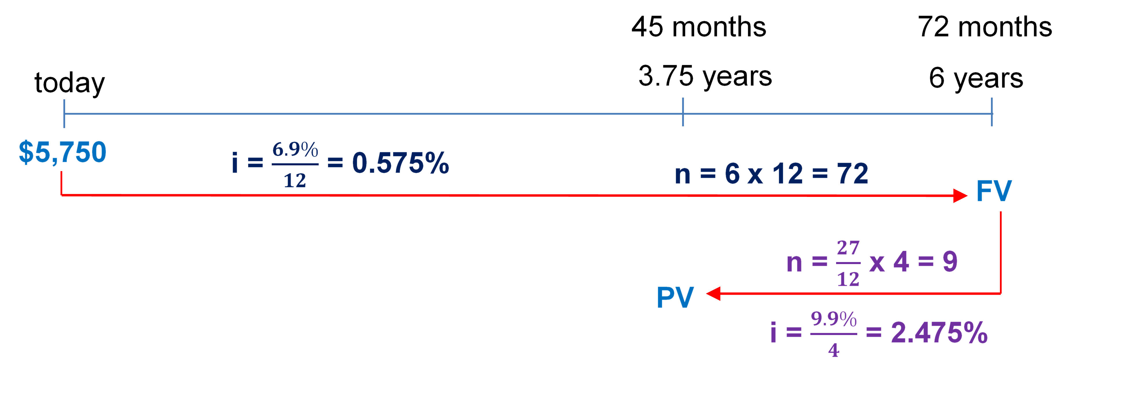

 \times (\text{Compounds Per Year}) = 6 \times 12 = 72")
^n\\ &= \$5,\!750(1+0.00575)^{72}\\ &= \$8,\!688.62 \end{align}")

 \times (\text{Compounds Per Year}) = \frac{27}{12} \times 4 = 9")
^n}\\ &=\frac{\$8,\!688.62}{(1.02475)^9}\\ &=\$6,\!972.52 \;\text{(Proceeds)} \end{align}")
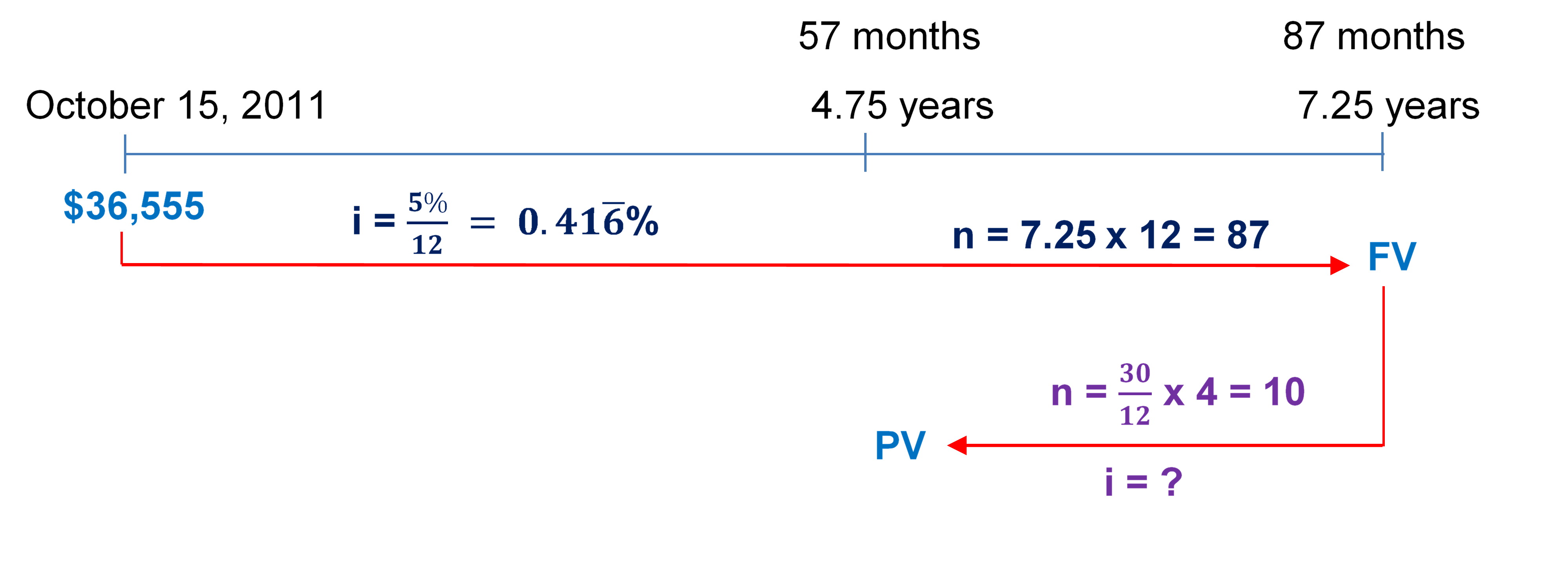

 \times (\text{Compounds Per Year}) = 7.25 \times 12 = 87")
^n\\ &= \$36,\!555(1+0.0041\overline{6})^{87}\\ &= \$52,\!486.97 \end{align}")
} \end{align}")
^n\\ \$52,\!486.97 &= \$40,\!753.56 (1+ i)^{10}\\ 1.287911 &= (1+ i)^{10}\\ (1.287911)^{(\frac{1}{10})} &= 1+ i\\ 1.025624 &= 1+ i\\ i &= 0.025624 \;\text{(rate per quarter)} \end{align}")
}\\ &= 0.025624 \times 4\\ &= 0.1025 \end{align}")

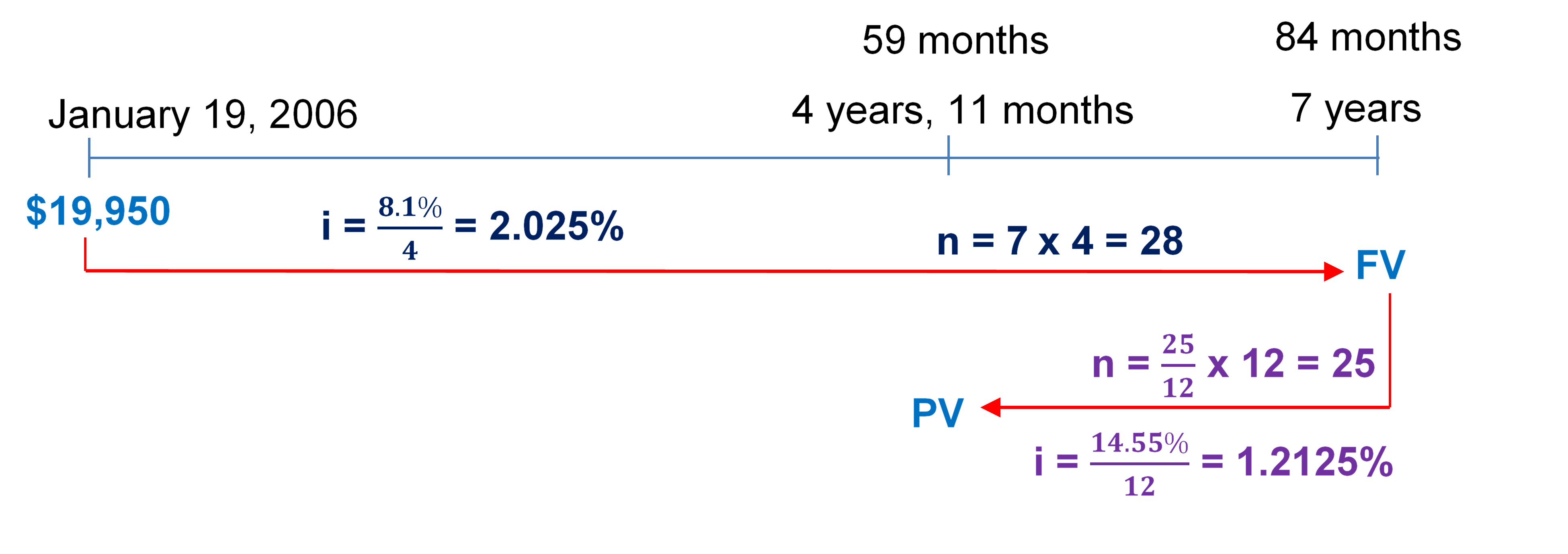

 \times (\text{Compounds Per Year}) = 7 \times 4= 28")
^n\\ &= \$19,\!950(1+0.02025)^{28}\\ &= \$34,\!972.59 \end{align}")
^n}\\ &=\frac{\$34,\!972.59}{(1.012125)^{25}}\\ &=\$25,\!874.62\;(\text{Proceeds}) \end{align}")

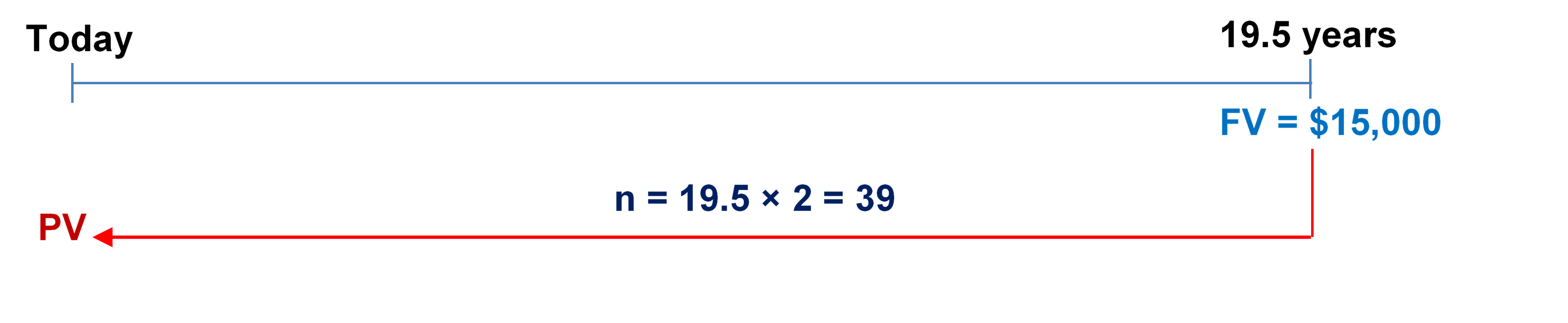
 ;
;  ;
;  ;
; 
 \times (\text{Compounds Per Year}) = 19.5 \times 2 = 39")

^n}\\ &=\frac{\$15,\!000}{(1.033661)^{39}}\\ &=\$4,\!124.24 \end{align}")
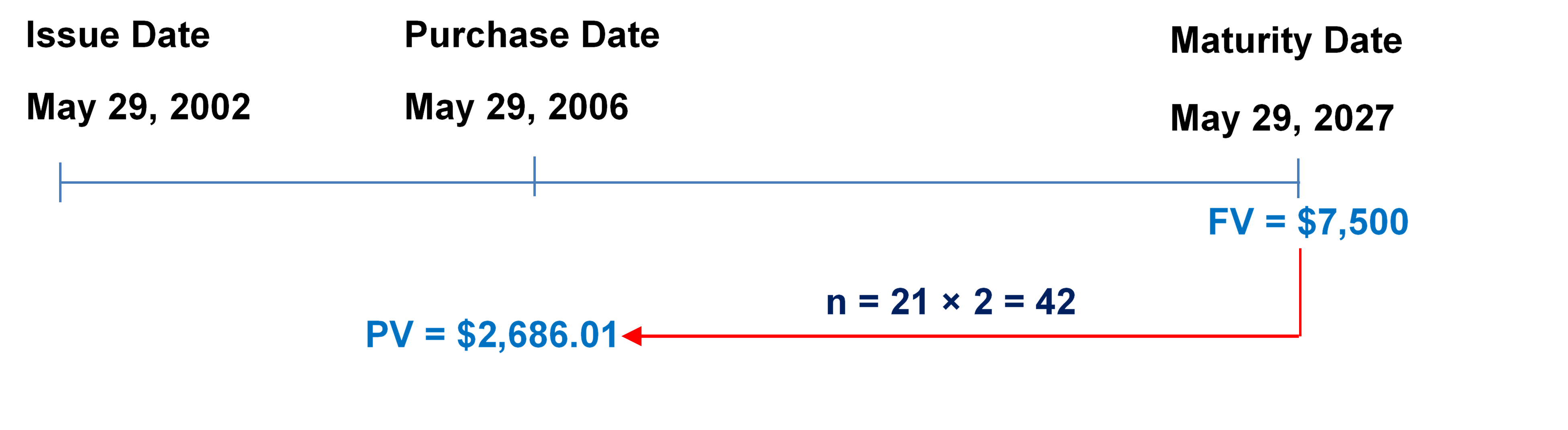
 ;
; 

^n\\ \$7,\!500 &= \$2,\!686.01 (1+ i)^{42}\\ 2.792246 &= (1+ i)^{42}\\ (2.792246)^{(\frac{1}{42})} &= 1+ i\\ 1.024750 &= 1+ i\\ i &= 0.024750 \;\text{(rate per half year)} \end{align}")
\\ &= 0.024750 \times 2\\ &= 0.0495 \end{align}")

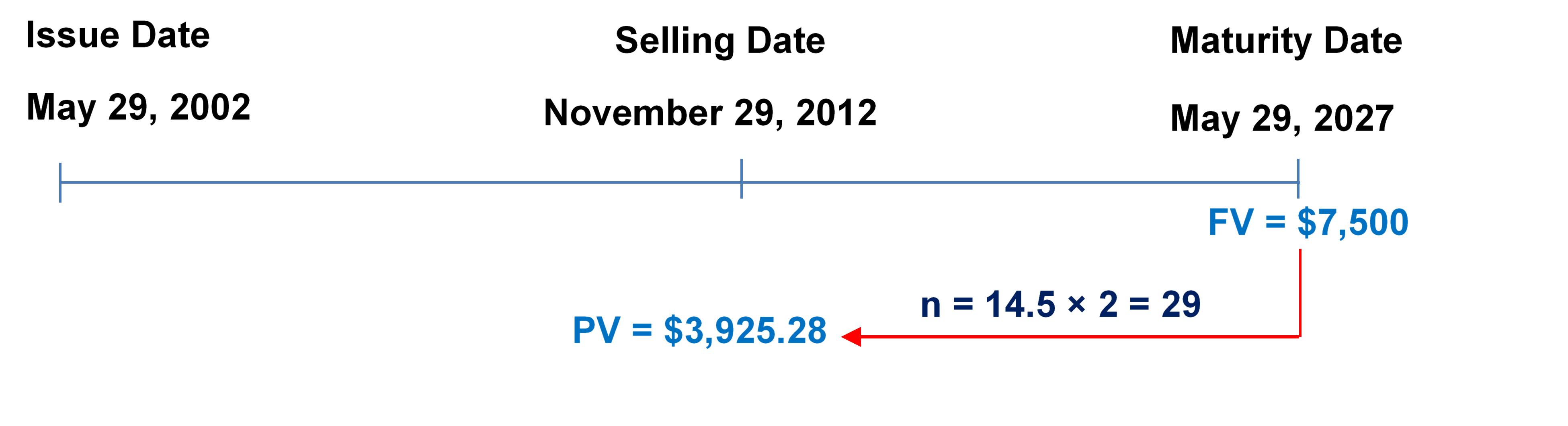
 ;
; 
^n\\ \$7,\!500 &= \$3,\!925.28 (1+ i)^{29}\\ i &= \left(\frac{\$7,\!500}{\$3,\!925.28}\right)^{\frac{1}{29}}-1\\ i &= 0.022577 \;\text{(rate per half year)} \end{align}")
\\ &= 0.022577 \times 2\\ &= 0.045155 \end{align}")

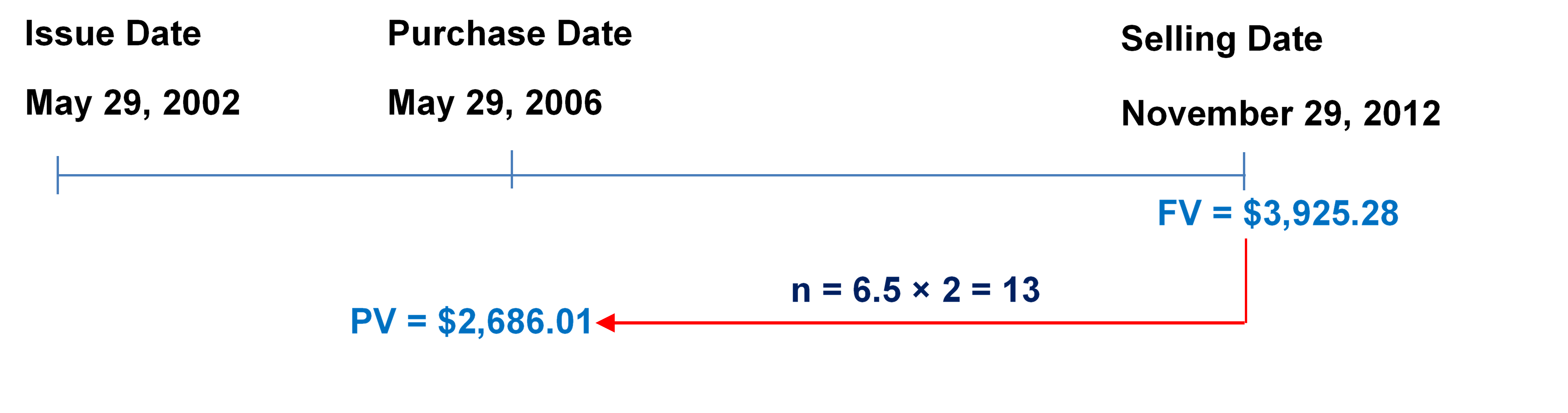


^n\\ \$3,\!925.28 &= \$2,\!686.01 (1+ i)^{13}\\ i &= \left(\frac{\$3,\!925.28}{\$2,\!686.01}\right)^{\frac{1}{13}}-1\\ i &= 0.029613 \;\text{(rate per half year)} \end{align}")
\\ &= 0.029613 \times 2\\ &= 0.059226 \end{align}")

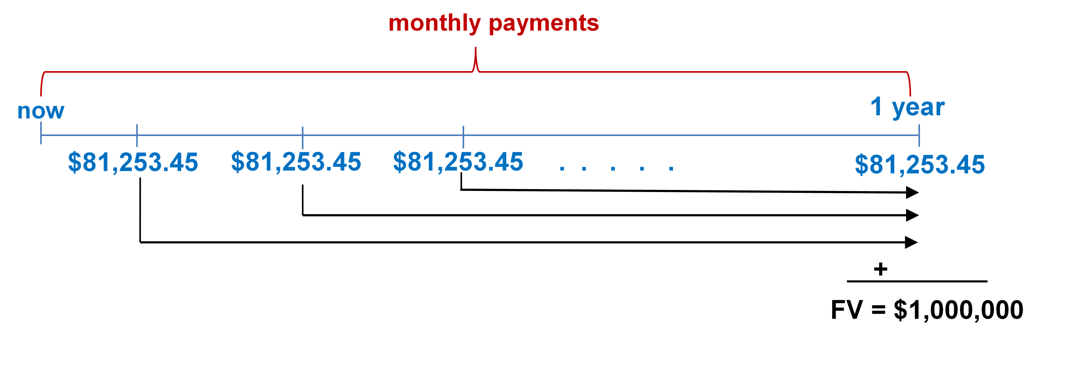
 ;
; 
 \times (\text{Payments Per Year})")

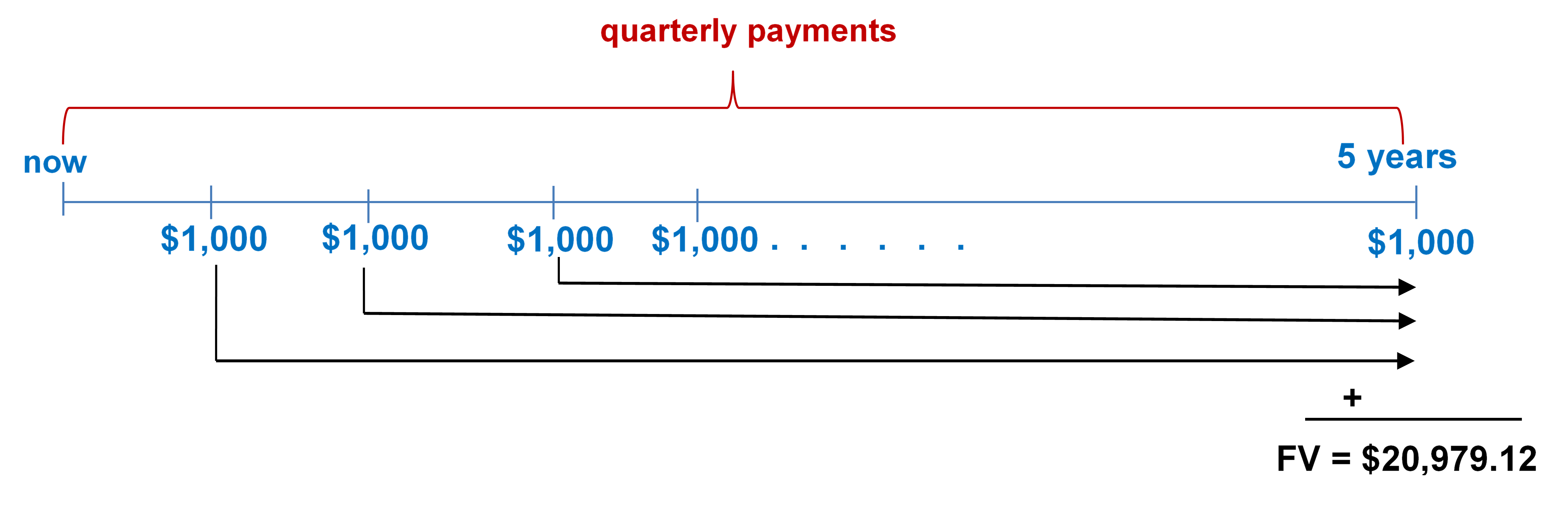
 ;
; 
 \times (\text{Payments Per Year})")

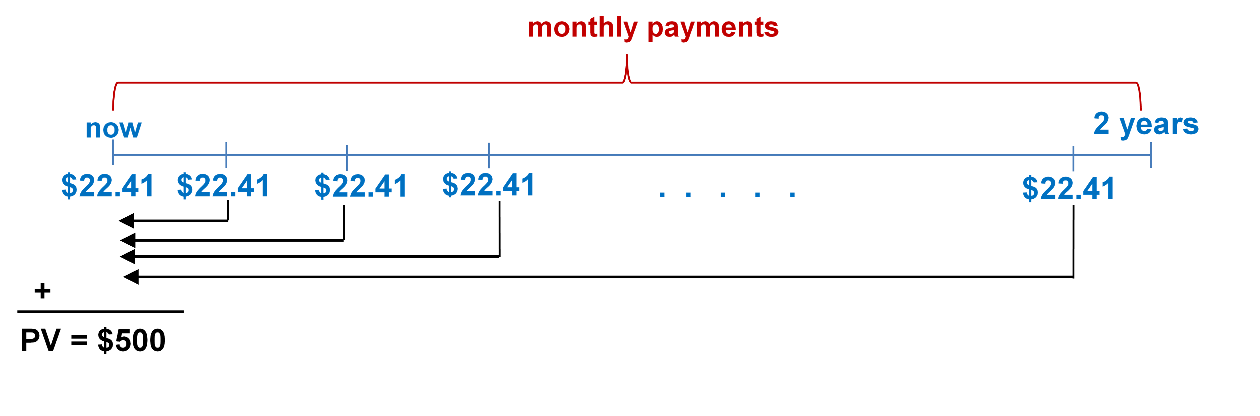
 ;
; 


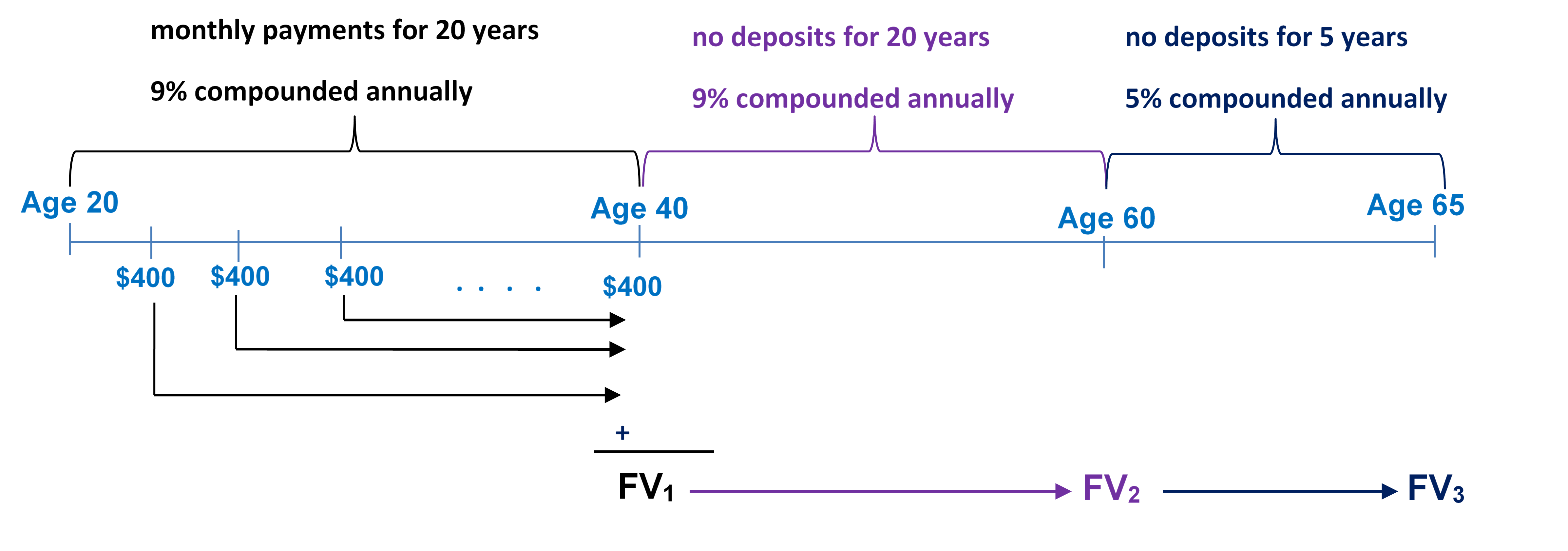


}")


}")


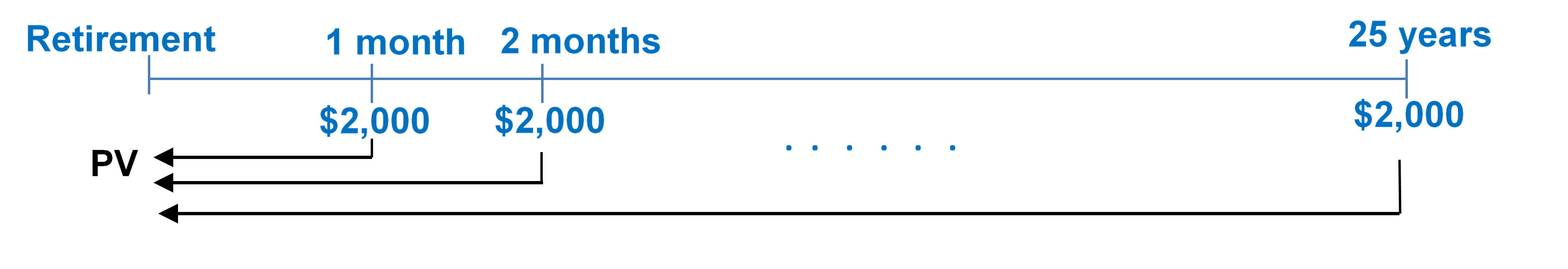


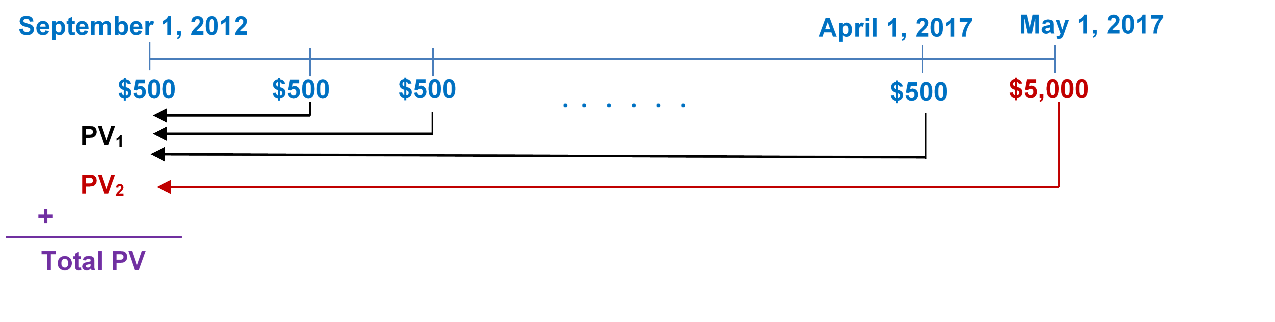
 – (\text{September}\; 1, 2012) = 4\frac{8}{12}")


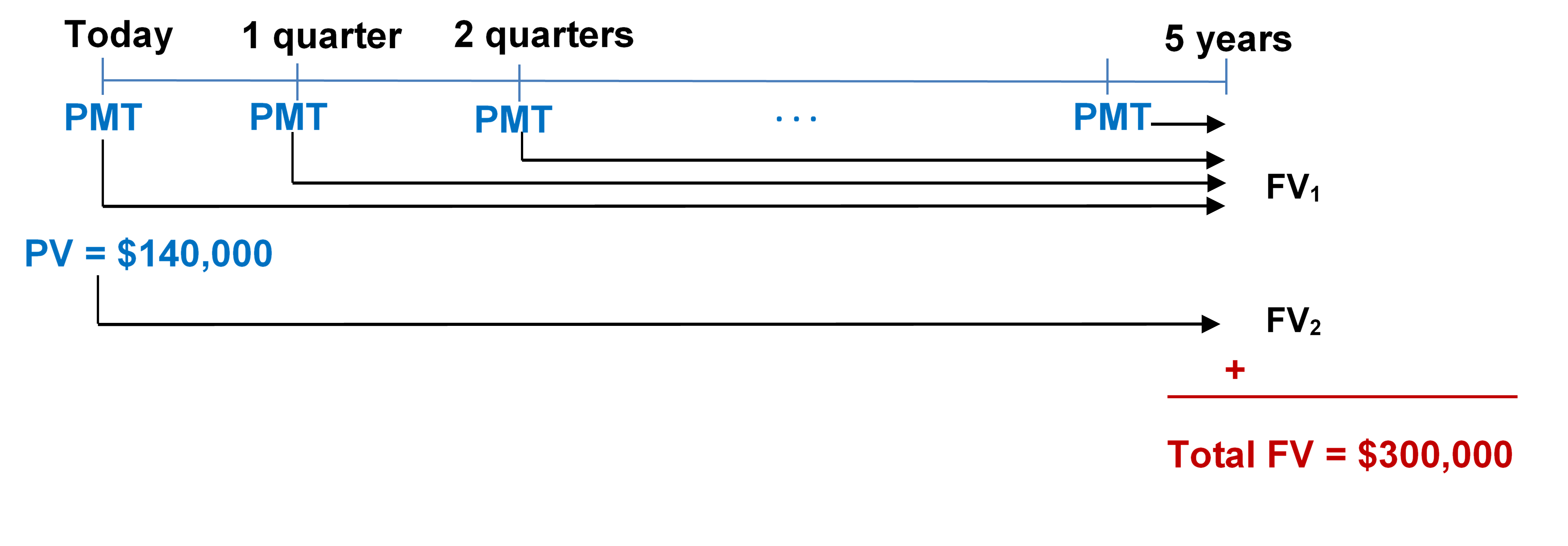


}")

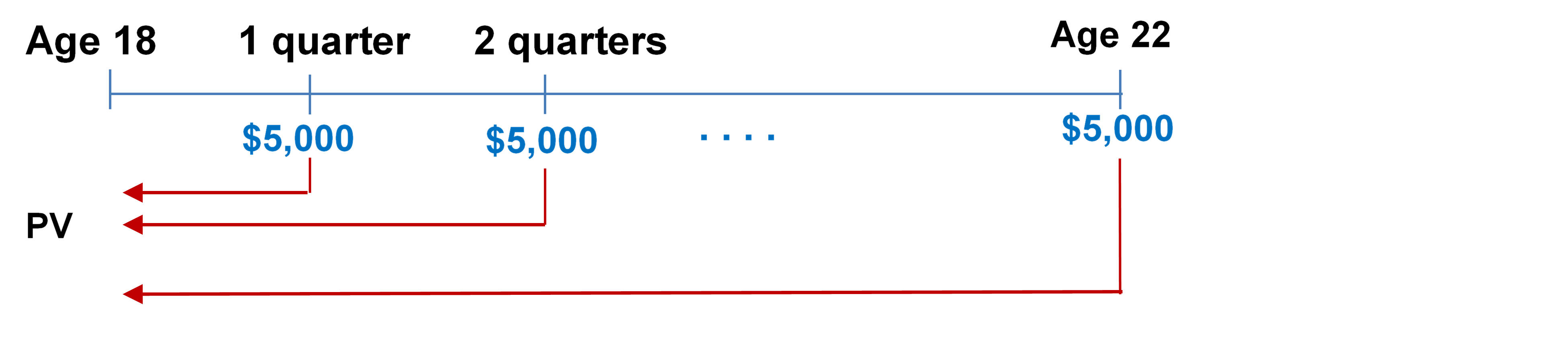


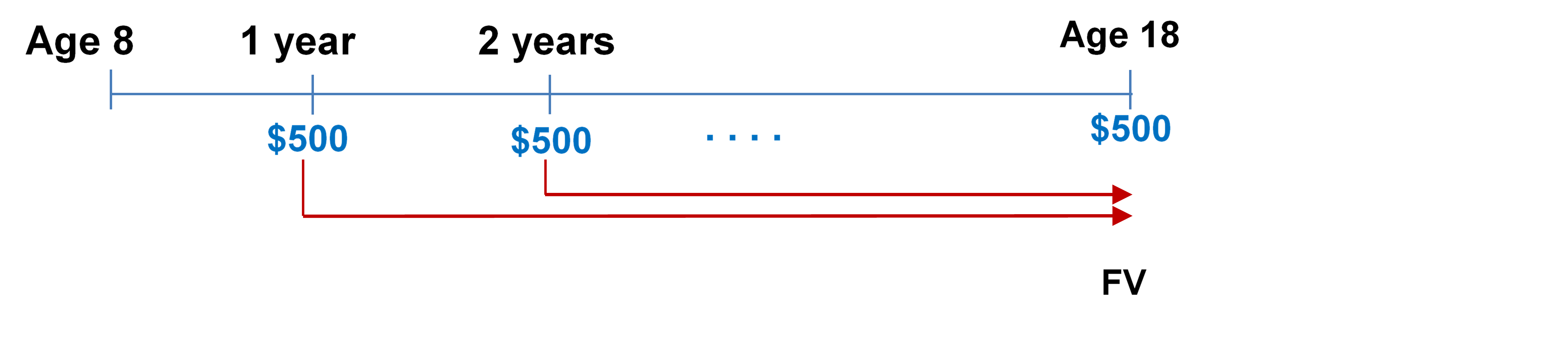


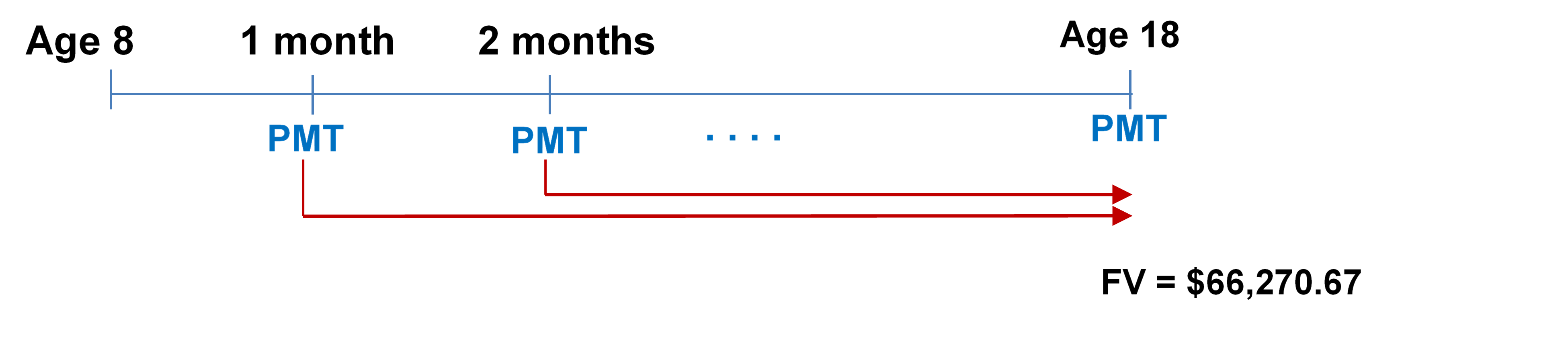


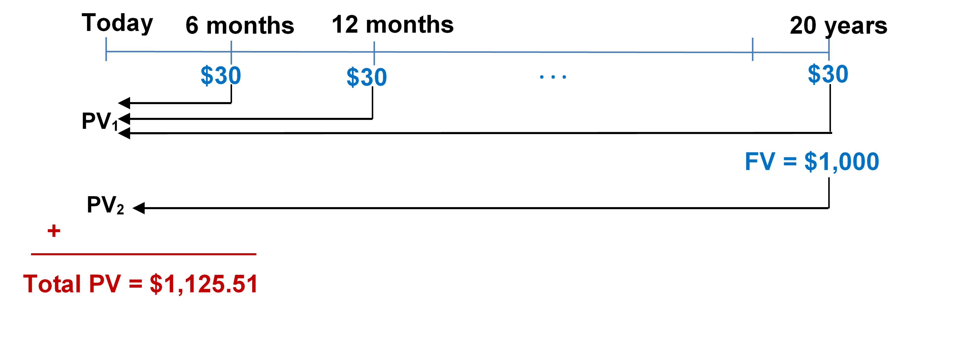


}")
}")


}")

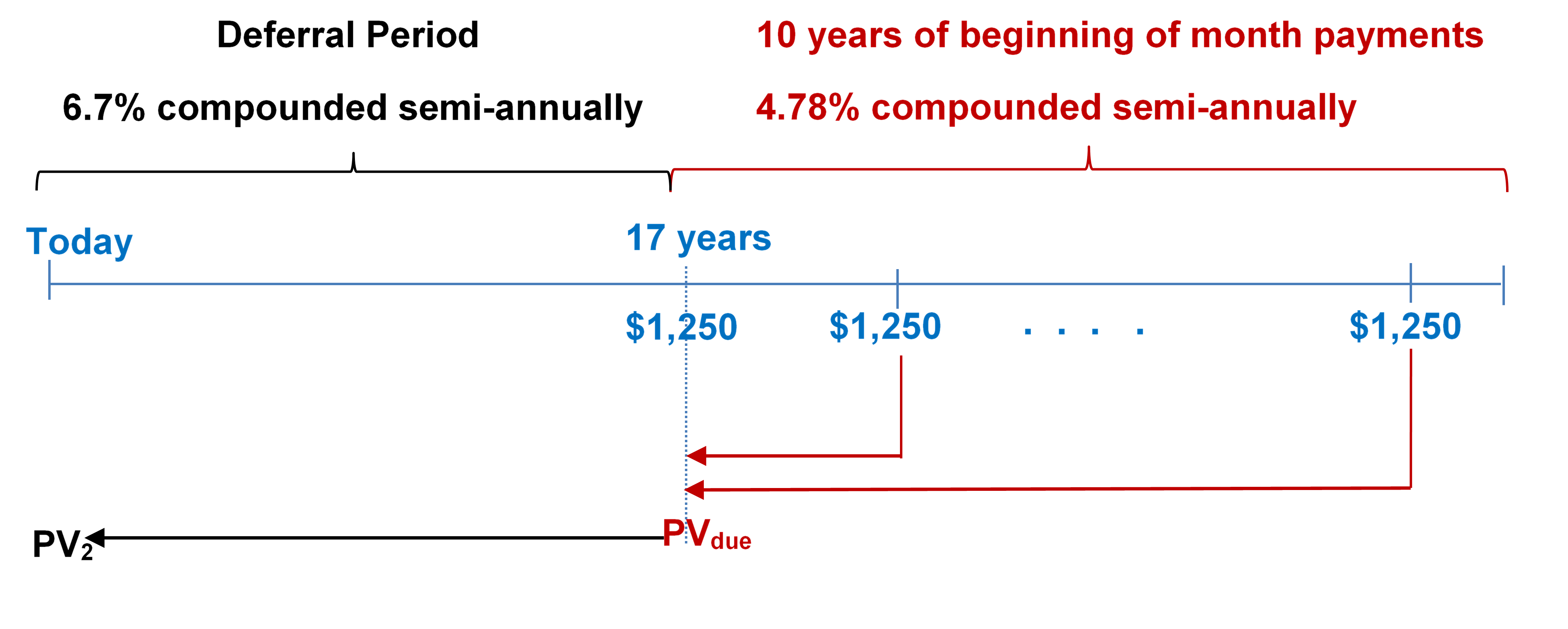
 .
.


}")
 .
.


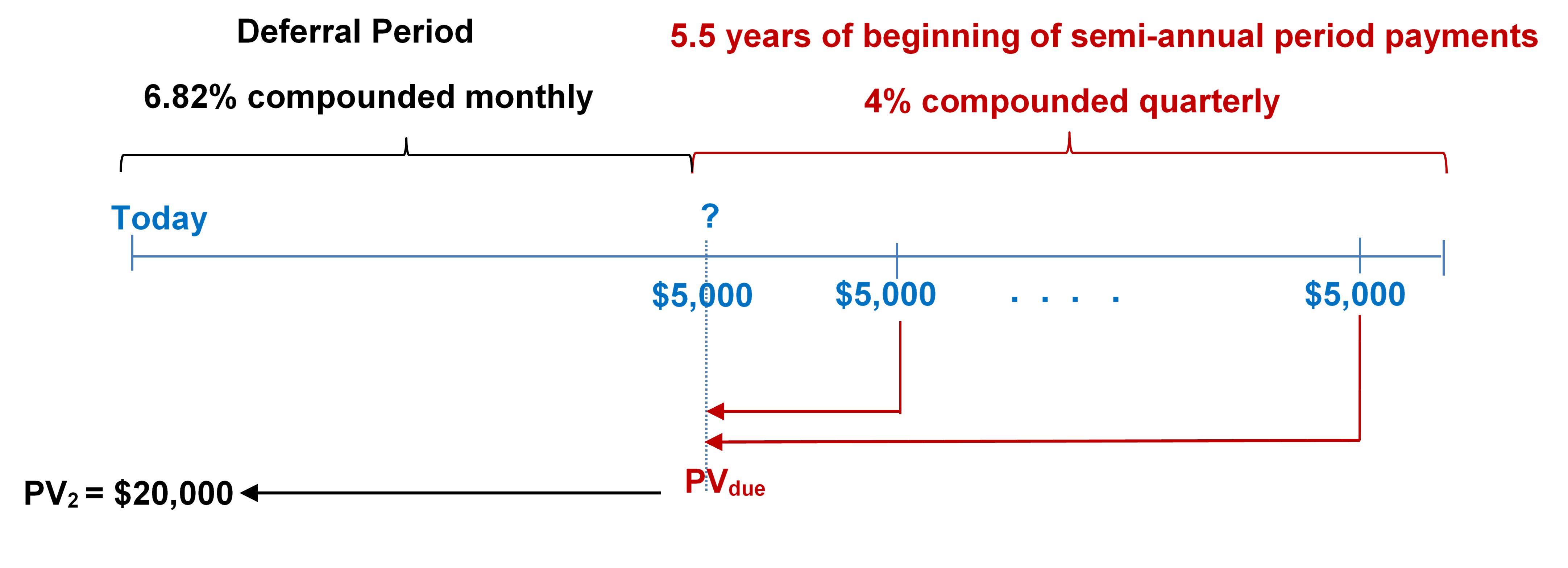


}")


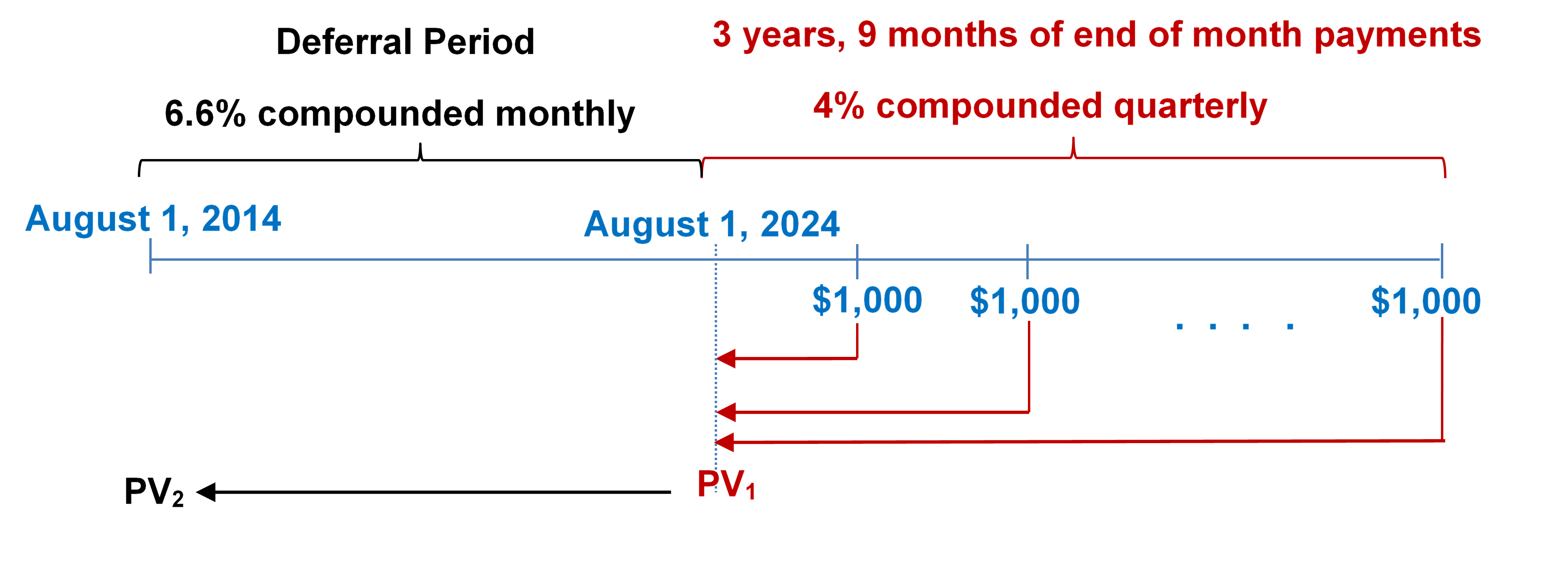


}")


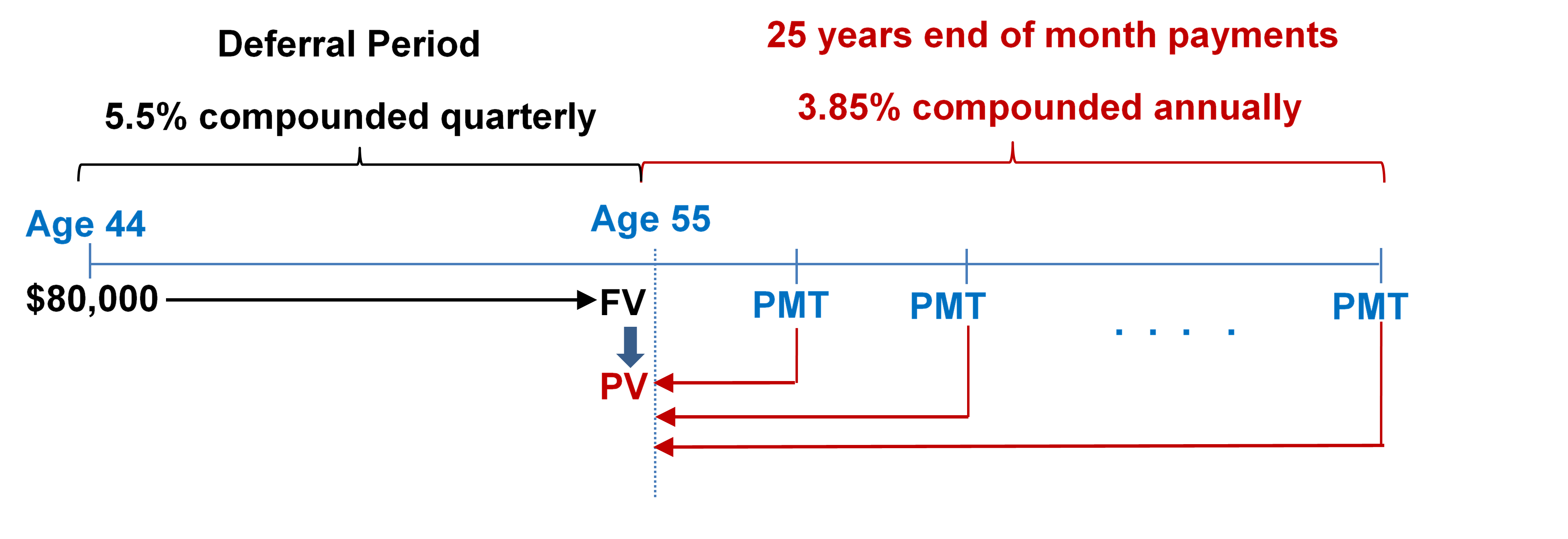


}")


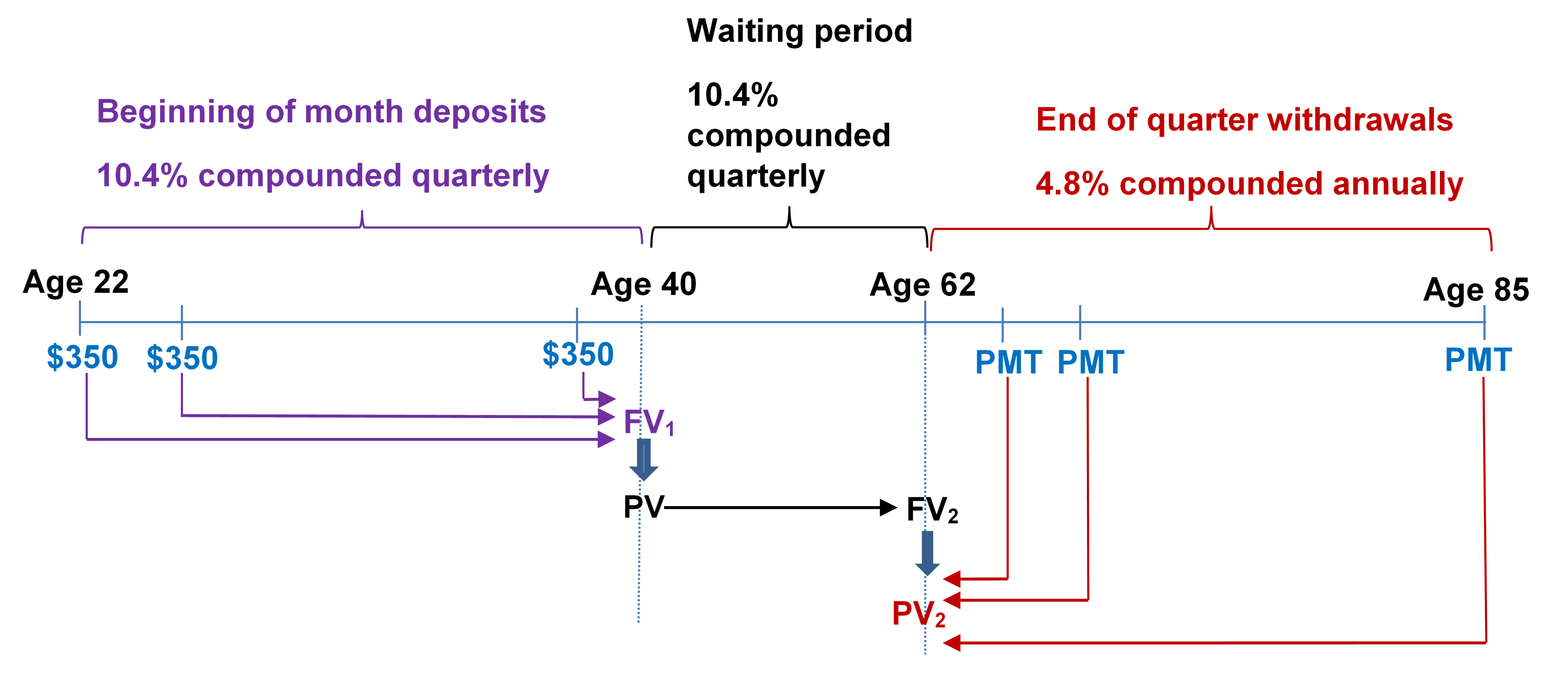


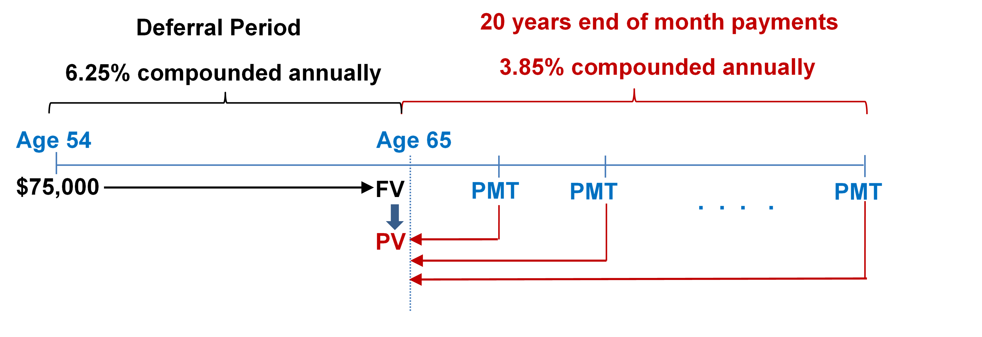


 + (60 \times 2,\!468.98) + (36 \times 2,\!953.71) - 188,\!321.26")
