Differential Equations

Amir Tavangar

eCampus Ontario

Differential Equations

Icon for the Creative Commons Attribution-NonCommercial-ShareAlike 4.0 International License

Preface

One or more interactive elements has been excluded from this version of the text. You can view them online here: https://ecampusontario.pressbooks.pub/diffeq/?p=4#oembed-3

About

This open-access textbook is designed to make the study of Differential Equations accessible and engaging for everyone. Differential Equations is a resource primarily intended for engineering students, but it’s versatile and beneficial for learners from any discipline. It serves as a comprehensive tool, whether you’re approaching differential equations for the first time or revisiting the topic for a refresher. Instead of delving into theorem proofs or formula derivations, the focus is on offering a step-by-step guide for solving differential equations.

Content and Format

Each chapter in this resource introduces essential concepts and provides illustrative examples with detailed solutions. Following these examples, there are ‘Try An Example’ questions to evaluate your comprehension. These questions are generated dynamically through MyOpenMath, enabling the generation of similar questions and providing immediate feedback to aid your learning process.

Incorporating interactive elements such as videos, dynamic problems, and graphs, the textbook is optimized for web viewing through Pressbook. This enables full interaction with its multimedia content, from watching instructional videos to engaging with dynamic graphs and problem sets. While a downloadable PDF version is available, it does not include the interactive features found in the web format.

Sponsor

This project has received support and funding from the Government of Ontario and eCampusOntario. The views expressed in this publication are the views of the author(s) and do not necessarily reflect those of the Government of Ontario.

Acknowledgements

I am grateful for the support and contributions that have made this resource possible. First and foremost, my thanks go to the Government of Ontario and eCampusOntario, whose funding and belief in the importance of accessible educational resources have been instrumental in bringing this project to fruition.

I am profoundly grateful to Dr. Mohammad Reza Peyghami for his expertise and thoughtful feedback, which have been instrumental in shaping this resource.

Special thanks are also due to two remarkable Engineering students, Jazel Paco and Minh Khanh Truong, for their keen insights and diligent review, which have significantly enhanced the quality and accuracy of this work.

I extend my gratitude to the myriad of scientists, mathematicians, and educators whose foundational work underpins the concepts and methods presented in this book. While citing all their contributions individually within the text is impractical, their collective efforts have been indispensable. The References section lists key resources that have been instrumental in shaping the content of this book.

Accessibility Statement

The web version of this textbook is fully compliant with the Accessibility for Ontarians with Disabilities Act (AODA) requirements and adheres to the Web Content Accessibility Guidelines (WCAG) 2.0, Level AA standards. Furthermore, it aligns with the comprehensive checklist provided in Appendix A: Checklist for Accessibility of the Accessibility Toolkit – 2nd Edition, ensuring it meets the highest standards of accessibility.

Designed with interactivity at its core, the textbook incorporates videos, dynamic problems, graphs, and simulations, making it ideally suited for online learning through Pressbook. Key accessibility features have been integrated into the web version to accommodate diverse learning needs:

The content is accessible to users of screen-reader technology, enhancing navigability and usability.
Keyboard navigation is supported throughout, allowing users to easily move through content without a mouse.
Formatting for links, headings, and tables is optimized for screen-reader compatibility.
Mathematical equations are presented in AsciiMath and rendered via MathJax to ensure they are accessible. The JAWS screen reader is recommended for the best experience in accessing these equations.
All images are accompanied by comprehensive descriptions, provided through text within the main content, alt-text, or detailed image descriptions. These extended alt-texts ensure that all visual information is conveyed clearly to users who rely on screen readers.
Color is not used as the sole means of conveying information, ensuring content is accessible to users with color vision deficiencies.
Video content includes captions to support users with hearing impairments.
The option to adjust font size is available, catering to users with visual impairments.
While a PDF version of the textbook is offered for download, it’s important to note that this format lacks the interactive elements present in the web version, which are central to the enhanced learning experience provided by the online resource.

This holistic approach to accessibility ensures that all learners, regardless of their physical abilities, can effectively engage with and benefit from the rich educational content provided in this textbook.

Introduction

Chapter Outline

This chapter provides an overview of fundamental concepts in differential equations along with an introduction to direction fields for first-order differential equations.

1.1 Introduction: This section covers basic definitions concerning differential equations, including their order, various classifications, and the nature of their solutions.

1.2 Direction Fields: This section briefly introduces direction fields, a tool for visually representing the behavior of solutions to first-order differential equations without needing an exact solution formula.

Pioneers of Progress

Madame Du Châtelet at her desk, detail — Émilie du Châtelet (1706 – 1749). Attribution: Maurice Quentin de La Tour, Public domain, via Wikimedia Common

Émilie du Châtelet, born in Paris in 1706, was a woman of exceptional intellect and determination who carved her unique path in the male-dominated world of science and mathematics during the Enlightenment. Despite societal norms restricting women’s access to formal education, Du Châtelet educated herself in mathematics and physics, often through creative means such as disguising herself as a man to attend lectures. Her most significant work, a translation and commentary on Isaac Newton’s ‘Principia Mathematica’, remains the standard French translation to this day. In it, she clarified Newton’s ideas and expanded on them, particularly in her elucidation of the principle of conservation of energy. Émilie du Châtelet’s work laid the groundwork for future developments in physics and mathematics, including those in differential equations. Her tenacity and brilliance broke through the constraints of her time, paving the way for future generations of women in science, and her legacy continues to inspire and challenge norms in the scientific community.

1.1 Introduction

A. Definitions

Differential equations (DEs) are mathematical equations that describe the relationship between a function and its derivatives, either ordinary derivatives or partial derivatives. In its simplest form, it describes the rate at which a quantity changes in terms of the quantity itself and its derivatives. Differential equations are powerful tools in mathematics and science as they enable the modeling of a wide range of real-world phenomena across various disciplines, including physics, engineering, biology, economics, and many others. Here are a few examples of differential equations.

Basic population growth: $(dP)/(dt)=aP$
Basic radioactive decay: $(dQ)/dt=-kQ$
Newton’s laws of cooling: $(dT)/(dt)=-k(T-T_m)$
Second Newton’s law of motion: $(d^2 y)/(dx^2 )=-g$
RL circuits: $L (dI)/(dt)+RI=E(t)$
RLC circuits: $L (d^2 I)/(dt^2 )+RI+1/C I=(dE)/dt$
Heat equation: $(del u)/(del t) =beta (del^2 u)/(del x^2)$

B. Order of Differential Equations

The order of a differential equation is the order of the highest derivative that appears in the equation. For example, if the highest derivative is a second derivative, the equation is of second order. Here are a few examples:

$dy/dx+3x^2=0$ (First Order)

$(d^2y)/dt^2 -2dy/dt + y= -5x$ (Second Order)

$x^2y'''+xy=cosx$ (Third Order)

$(del u)/(del t)=5(del^2 u)/(del t^2)$ (Second Order)

The order of a differential equation often determines the methods used to solve it. The order of a differential equation is independent of the type of derivatives involved, whether they are ordinary or partial derivatives.

Throughout this book, our focus will primarily be on first- and second-order differential equations. As you’ll discover, the methods used to solve second-order differential equations can often be easily extended to tackle higher-order equations.

Try an Example

One or more interactive elements has been excluded from this version of the text. You can view them online here: https://ecampusontario.pressbooks.pub/diffeq/?p=5

C. Ordinary and Partial Differential Equations

If an equation includes the derivative of one variable with respect to another, such as $dy/dt$ , then the variable whose derivative is taken (in this case, $y$ ) is known as the dependent variable. The variable with respect to which the derivative is taken (here, $t$ ) is called the independent variable.

An Ordinary Differential Equation (ODE) is a differential equation involving a function of one independent variable and its derivatives. All the above examples except the heat equation are ordinary differential equations.

A Partial Differential Equation (PDE) is a differential equation that contains unknown multivariable functions and their partial derivatives. PDEs are used to formulate problems involving functions of several variables.

In this textbook, our primary focus will be on ordinary differential equations, which involve functions of a single variable. We will only delve into partial differential equations in the final chapter.

D. Linear and nonlinear Differential Equations

A linear differential equation is one in which the dependent variable $y$ and its derivatives appear with the first power, are not multiplied together, and are not arguments of another function, e.g., $sin(y)$ or $ln(y')$ . The general form of a linear differential equation is

$a_n(x) (d^ny)/dx^n+a_(n-1)(x) (d^(n-1) y)/dx^(n-1)+$ $...+a_1(x) (dy)/dx+a_0(x)y=f(x)$

where $y$ is the dependent variable, $x$ is the independent variable, $a_i(x)$ are functions of $x$ (which can be constants or zeros), and $f(x)$ is a function of $x$ .

A nonlinear differential equation is one in which the dependent variable or its derivatives appear to a power greater than one, or they are multiplied together, or in any way that does not fit the linear form. For example, $dy/dx+3y^2=3x$ is nonlinear since $y^2$ has a power of 2.

Try an Example

One or more interactive elements has been excluded from this version of the text. You can view them online here: https://ecampusontario.pressbooks.pub/diffeq/?p=5

E. Homogeneous and Nonhomogeneous Differential Equations

A differential equation is termed homogeneous if every term in the equation is a function of the dependent variable and its derivatives. For linear differential equations, an equation is homogeneous if the function $f(x)$ on the right-hand side of the equation is zero.

$a_n(x) (d^ny)/dx^n+a_(n-1)(x) (d^(n-1) y)/dx^(n-1)+$ $...+a_1(x) (dy)/dx+a_0(x)y=0$

For example, the linear equation $(d^2 y)/(dx^2 )+3 (dy)/(dx)+2y=0$ is homogeneous because all terms are functions of $y$ and its derivatives, and the equation equals zero.

A differential equation is nonhomogeneous if it includes terms that are not solely functions of the dependent variable and its derivatives. For linear equations, this typically means there is a non-zero function on the right-hand side of the equation. For example, the linear equation $(d^2 y)/(dx^2 )+3 (dy)/(dx)+2y=xe^x$ is nonhomogeneous because of the presence of the term $xe^x$ , which is a function of the independent variable $x$

F. Solutions

A solution of a differential equation is a function that satisfies the equation on some open interval. This means that when the function and its derivatives are plugged into the differential equation, the equation holds true for all values within the interval. Often there are a set of solutions.

Example 1.1.1: Verify Solution

Verify $y = sin(2x) + x^2$ is a solution to $y'' + 4y = 2+4x^2$ .

Show/Hide Solution

First, we find $y''$ since it appears in the equation:

$y'=2cos(2x)+2x$ " title="->" class="asciimath mathjax"> $y''=-4sin(2x)+2$ .

By substituting $y''$ and $y$ into the left-hand side of the equation, we obtain

$LHS:$

$-4sin(2x)+2+4sin(2x)+4x^2$

$=2+4x^2$

which is equal to the right-hand side of the equation. Since the given $y$ satisfies the equation, it is a solution to the equation.

Try an Example

One or more interactive elements has been excluded from this version of the text. You can view them online here: https://ecampusontario.pressbooks.pub/diffeq/?p=5

Now, consider the differential equation $y' = 3x^2$ . We can easily solve this equation by integrating:

$dy/dx=3x^2$

$dy=3x^2dx$

$int dy=int3x^2dx$

$y=x^3+C$

$y=x^3+C$ , where $C$ is an arbitrary constant, represents a family of solutions to the given differential equation. Each distinct value of $C$ yields a unique particular solution, demonstrating how various initial conditions can be satisfied. This family of solutions, encompassing all possible solutions through the inclusion of the arbitrary constant $C$ , is known as the general solution of the differential equation.

An explicit solution explicitly expresses the dependent variable in terms of the independent variable(s). For example, $y=x^3+C$ is an explicit solution. On the other hand, an implicit solution, may not directly express the dependent variable explicitly but still satisfies the differential equation. An example is $y^2+x^2=C$ Note that finding an explicit solution is not always possible.

G. Initial Conditions

Initial condition(s) refer to the values specified for the dependent variable and possibly its derivatives at a specific point. Initial conditions are used to determine the specific (or particular) solution of a differential equation from the general solution, which typically contains arbitrary constants. For example, $y(t_0)=y_0$ states that at time $t_0$ , the value of $y$ is $y_0$ . The number of initial conditions required for a given differential equation depends on the order of the differential equation. Generally, an $nth$ order differential equation needs $n$ initial conditions. These conditions specify the values of the function and its derivatives up to the $(n-1)th$ order at a particular point. For example, a second-order differential equation requires two initial conditions. These are often the value of the function and the value of its first derivative at a specified point.

An Initial Value Problem (IVP) is a differential equation with initial condition(s) that nails down one particular solution. A solution might not be valid for all real numbers – there is the “interval of validity” or the domain of the solution.

Example 1.1.2: Inital Value Problem

$y'=3x^2$ , $y(1)=2$ is an initial value problem, where $x=1$ and $y=2$ can be substituted in the general solution of $y=x^3+C$ to find $C$ , which results in the particular solution of $y=x^3+1$ .

1.2 Direction Fields

Although having an explicit formula for the solution of a differential equation is useful for understanding the nature of the solution, determining where it increases or decreases, and identifying its maximum or minimum values, finding such a formula is often impossible for most real-world differential equations. Consequently, alternative methods are employed to gain insights into these questions. One effective approach for visualizing the solution of a first-order differential equation is to create a direction field for the equation. This method provides a graphical representation of the solution’s behavior without requiring an explicit formula.

We assume that the first-order differential equation $y'=f(x,y)$ has solutions. For this equation, function $f(x,y)$ gives the slope of the solution curve at any point $(x,y)$ in the XY-plane. In a direction field, these slopes are represented by small line segments or arrows, drawn at a selection of points in the plane. Each segment has a slope equal to the value of $f(x,y)$ at that point.

Example 1.2.1: Compute FV

For the equation $dy/dx=x+y$ , the graph of the solution passing through the point $(-1, 3)$ must have a slope of $dy/dx=-1+3=2$ .

The general solution of the equation is $y=-x-1+Ce^x$ . The direction field and some of the solutions of the equation for different values for constant $C$ are shown in Fig. 1.2.1.

One or more interactive elements has been excluded from this version of the text. You can view them online here: https://ecampusontario.pressbooks.pub/diffeq/?p=89

Figure 1.2.1 Direction field for and solutions to $y'=x+y$

The arrows in the direction fields represent tangents to the actual solutions of the differential equations. We can use these arrows as guides to sketch the graphs of the solutions to the differential equation, providing a visual representation of how the solutions behave. By following these arrows, we can visually trace the trajectory of a solution over time, which can indicate its long-term behavior.

First Order Differential Equations

Chapter Outline

This chapter delves into first-order differential equations, vital in science and engineering for modeling rates of change in numerous phenomena. It covers their structure, solution techniques, and real-world applications in fields like population dynamics, thermal processes, and electrical circuits.

2.1 Separable First-Order Differential Equations: This section addresses separable differential equations, a category of first-order equations where each variable can be separated on different sides of the equation.

2.2 Linear First-Order Differential Equations: This section covers the solution to first-order nonhomogeneous linear equations.

2.3 Exact Differential Equations: This part explains the criteria for an equation to be exact and outlines methods for solving these equations.

2.4 Integrating Factors: This section explores the techniques of utilizing integrating factors to transform a non-exact equation into an exact equation that can be solved.

2.5 Applications of First-Order Differential Equations: The final section illustrates the use of first-order differential equations in modeling growth and decay, substance mixing, temperature changes, motion under gravity, and circuit behaviors.

Pioneers of Progress

Mary Cartwright (1900-1998) Credit: Anitha Maria S, CC BY-SA 4.0 <https://creativecommons.org/licenses/by-sa/4.0>, via Wikimedia Commons

Mary Cartwright, born in 1900 in Aynho, Northamptonshire, England, emerged as a pioneering mathematician in an era when female academics were a rarity. Her journey in mathematics began at Oxford University, leading her to Cambridge, where she initially focused on classical analysis. However, it was during World War II, while investigating the problem of radio waves and their interference patterns, that Cartwright made a groundbreaking discovery. Collaborating with J.E. Littlewood, she delved into nonlinear differential equations, and their work laid the foundational stones for what would later be known as chaos theory. Cartwright’s foray into this field produced seminal results, including the Cartwright-Littlewood theorem and her study of the Van der Pol oscillator, a concept critical in the understanding of oscillatory systems. Her extraordinary contributions not only advanced the field of mathematics but also broke gender barriers, setting a precedent for women in STEM. Mary Cartwright’s life was a blend of intellectual rigor and quiet resilience, inspiring a legacy that continues to encourage mathematicians, especially women, to explore and reshape the boundaries of mathematical knowledge.

2.1 Separable Equations

Separable equations are a type of first-order differential equations that can be rearranged so all terms involving one variable are on one side of the equation and all terms involving the other variable are on the opposite side. This characteristic makes them easier to solve compared to other types of differential equations. Often, these equations represent nonlinear relationships.

Understanding and applying integration techniques is crucial for solving separable equations. Therefore, reviewing and familiarizing yourself with standard integration methods is recommended before attempting to solve these equations.

Solution to Separable Differential Equation

A first-order differential equation is called separable if it can be written in the form of

$dy/dx = g(x) p(y)$

where $g(x)$ is a function of $x$ only and $p(y)$ is a function of $y$ only. The right-hand side is a product of these two functions, allowing the separation of variables.

For example, the equation $y'=(x^2+x^2y)/y^2$ is separable as it can be factored in and written as $dy/dx=x^2((1+y)/y^2)=g(x)p(y)$ . However, the equation $y'=2-x^2y$ is not separable as the right-hand side cannot be factored into a product of the functions of $x$ and $y$ .

How to Solve Separable Equations

To solve the equation $dy/dx = g(x) p(y)$ ,

1. Separate variables: multiply both sides by $dx$ and by $h(y)=1/(p(y))$ " title="->" class="asciimath mathjax"> $h(y)dy=g(x)dx$

2. Integrate both sides: $inth(y)dy=intg(x)dx$ " title="->" class="asciimath mathjax"> $H(y)=G(x) +C$ where $C$ is the merged constant of integration.

3. Solve for $y$ : If possible, solve the resulting equation for $y$ to get the explicit solution. Some solutions cannot be rearranged and solved for $y$ , so the implicit form obtained in Step 2 may be the final solution.

Watch Video

One or more interactive elements has been excluded from this version of the text. You can view them online here: https://ecampusontario.pressbooks.pub/diffeq/?p=138#oembed-3

Example 2.1.1: Solve a Separable Equation

Solve the nonlinear equation

$y'=(x+4)/y^2$ .

Show/Hide Solution

1. Multiplying both sides by $dx$ and $y^2$ we get

$y^2dy=(x+4)dx$

2. Integrating both sides, we get

$inty^2dy=int(x+4)dx$

$y^3/3=x^2/2+4x+C_1$

3. Multiplying by 3 and taking the cubic root of both sides, we obtain

$y=((3x^2)/2+12x+3C_1)^(1//3)$

By substituting constant $C_2=3C_1$ , we’ll have the explicit solution

$y=((3x^2)/2+12x+C_2)^(1//3)$

Example 2.1.2: Solve a Separable Equation

Solve the differential equation

$dy/dx =6y tan^2(2x)$ .

Show/Hide Solution

This is a separable differential equation as it can be expressed in the form $h(y) dy=g(x) dx.$

1. Multiplying both sides by $dx$ and $1/y$ we obtain

$1/(y)dy = 6tan^2(2x)dx$

2. Integrating both sides, we get

$int 1/(y) dy= int 6 tan^2(2 x) dx$

$ln|y| = 3tan(2x)-6x+C_1$

3. Exponentiating both sides yields

$y= C_2e^(3tan(2x)-6x)$ where $C_2=e^(C_1)$

Try an Example

One or more interactive elements has been excluded from this version of the text. You can view them online here: https://ecampusontario.pressbooks.pub/diffeq/?p=138

When solving nonlinear differential equations using the separable method, it is crucial to consider the interval of validity, which is the range of the independent variable, typically $x$ , where the solution is defined and behaves appropriately. This interval is essential because solutions to nonlinear equations may not be valid across all $x$ values due to potential issues like division by zero, undefined logarithms of non-positive numbers, and other undefined operations.

Additionally, due to the nature of nonlinear equations, certain initial conditions might lead to no solution or multiple solutions, emphasizing the need to carefully select and verify the range of $x$ over which the solution is applicable. The interval of validity is not always immediately apparent from the equation itself and often depends on both the specific form of the solution and the initial conditions.

Example 2.1.3: Solve a Separable Equation with Initial Condition

Solve the initial value problem

$y'=14xy-2x$ , $y(0)=4.$

Show/Hide Solution

Find the general solution:

After factoring out $2x$ in the right-hand side, the equation can be expressed in the form $h(y) dy=g(x) dx.$

$(dy)/(dx)=2x(7y-1)$

1. Multiplying both sides by $dx$ and $1/(7y-1)$ we get

$dy/(7y-1)=2xdx$

2. Integrating both sides, we get

$intdy/(7y-1) =int2xdx$

$1/7ln|7y-1|=x^2+C_1$

3. Multiplying by 7 and exponentiating both sides, we obtain

$7y-1=e^(7x^2+7C_1)$

By rearranging the equation and substituting $C_2=e^(7C_1)$ , we’ll have the explicit solution

$y=1/7(C_2e^(7x^2)+1)$

Applying the initial condition:

$y(0)=4$

$1/7(C_2e^0+1)=4$

$C_2+1=28$

$C_2=27$

The solution to the IVP problem is then

$y=1/7(27e^(7x^2)+1)$

There is no restriction on the domain of $y$ , and therefore the solution is valid on $(-oo,oo)$ .

Try an Example

One or more interactive elements has been excluded from this version of the text. You can view them online here: https://ecampusontario.pressbooks.pub/diffeq/?p=138

Example 2.1.4: Solve a Separable Equation with Initial Condition

Solve the initial value problem and find the interval of validity of the solution.

$(dy)/(dx)=(5y^2)/(sqrt(x))$ , $y(4)=1/35.$

Show/Hide Solution

Find the general solution:

This is a separable differential equation as it can be expressed in the form $h(y) dy=g(x) dx.$

1. Multiplying both sides by $dx$ and $1/(y^2)$ we get

$1/(y^2)\ dy=5/(sqrt(x))\ dx$

2. Integrating both sides, we get

$inty^-2\ dy =5intx^(-1/2) \ dx$

$-y^-1=10x^(1/2)+C$

3. Multiplying by -1 and taking the reciprocal of both sides, we obtain the explicit solution

$y=-1/(10sqrt(x)+C)$

Applying the initial condition:

$y(4)=1/35$

$-1/(10sqrt(4)+C) =1/35$

$-1/(20+C) =1/35$

$20+C=-35$

$C=-55$

The solution to the IVP problem is then

$y=-1/(10sqrt(x)-55)$

Find the interval of validity:

To establish the interval of validity for the solution, we need to consider two constraints:

The expression within a square root must be positive. Therefore, the term under the square root, should be greater than or equal to 0 (=0" title="x>=0" class="asciimath mathjax">).
The denominator of any rational function should not equal zero to avoid undefined expressions. Given $10sqrt(x)-55!=0$ , it implies that $x!=+-30.25$ .

The interval of validity is the range of $x$ values that satisfy both conditions:

Try an Example

One or more interactive elements has been excluded from this version of the text. You can view them online here: https://ecampusontario.pressbooks.pub/diffeq/?p=138

Section 2.1 Exercises

Solve the differential equation: $dy/dx =4cos(3x) sqrt(1-y^2)$

Show/Hide Answer

$y(x)=sin(4/3sin(3x)+C)$
Solve the differential equation. Express $y$ explicitly as a function of $x$ .
$dy/dx =4 e^(5x) e^(4y)$

Show/Hide Answer

$y(x)=-1/4lnabs(-16/5 e^(5x)+C)$
Solve the initial value problem: $y' = 4x y-2x ,$ $y(0)=3$

Show/Hide Answer

$y(x)=(5 e^(2x^2)+1)/2$
Solve the initial value problem and find the interval of validity of the solution: $(dy)/(dx) = (3 y^2)/sqrt(x), \ \ \ y(4) = 1/42$

Show/Hide Answer

$y(x)=-1/(6 sqrt(x) -54)$

Interval of validity: $[0,81)uu(81,oo)$

2.2 Linear First-Order Differential Equations

A first-order differential equation is classified as linear if it can be written as

$y' + p(x) y = q(x)$ . (2.2.1)

A first-order differential equation that cannot be expressed in that form is called nonlinear. If $q(x)=0$ , the equation is said to be homogeneous. In contrast, if $q(x)$ is not zero, the equation is nonhomogeneous. Homogeneous equations always have the trivial solution $y=0$ . Solutions that are not zero are referred to as nontrivial solutions.

Some equations may not appear to be linear at first, such as $x^3 y' + ln(x) y = 2sin(x)$ but can be rearranged into the standard linear form:

$y'+ln(x)/x^3 y = (2sin(x))/x^3$ .

Theorem: If $p(x)$ and $q(x)$ in Equation 2.2.1 are continuous on some open interval (a,b), then there’s a unique formula $y = y(x,c)$ that is the general solution to the differential equation.

In our discussions within this text, we will not always explicitly mention the interval $(a,b)$ when seeking the general solution of a specific linear first-order equation. By default, this implies that we are looking for the general solution on every open interval where the functions $p(x)$ and $q(x)$ in the equation are continuous.

To solve Equation 2.2.1, we start by assuming that the solution can be expressed as , where is a known solution to the corresponding homogeneous equation (called complementary equation), and $v(x)$ is an unknown function we aim to determine. This approach is part of a technique called variation of parameters, which is particularly useful for finding solutions to nonhomogeneous differential equations. We will explore this technique more thoroughly in the context of second-order differential equations. Substituting the guessed solution into the equation yields

$v'y_1+y'_1v+p(x)(vy_1)=q(x)$

By simplifying and rearranging, we obtain

$v'y_1+v(y'_1+p(x)y_1)=q(x)$

Since is a solution to the complementary equation, , simplifying the expression to . Integrating both sides allows us to determine $v(x)=int(q(x))/(y_1(x))dx+C$ , leading to the solution for Equation 2.2.1 as

Now that we understand the derivation of the solution, let’s outline the solution process in the following steps.

How to Solve Linear First-Order Equations

1. Write the equation in the standard form.

$dy/dx + p(x) y = q(x)$

2. Calculate the integrating factor letting the constant of integration be zero for convenience.

$u(x)=e^(int p(x) dx)$

3. Integrate the right-hand side equation and simplify where possible. Ensure you properly deal with the constant of integration.

$y(x)=1/(u(x))[int u(x)q(x)dx+C]$

Occasionally, the function $u(x)$ may not be integrable in a straightforward manner. In that case, it is necessary to retain the function in its integral form instead of attempting to find an explicit solution.

Example 2.2.1: Solve a Linear Equation

Find the general solution to

$1/x dy/dx-(2y)/x^2=xcosx$ , 0" title="x>0" class="asciimath mathjax">

Show/Hide Solution

1. First, we multiply by $x$ to put the equation in the standard form:

$dy/dx-2/x y=x^2cosx$

So $p(x)=-2/x$ and $q(x)=x^2cosx$

2. Thus, the integrating factor is

$u(x)=e^(int p(x)dx)=e^(int -2/x dx)=e^(-2ln|x|)=x^-2$

3. Substituting into the general formula, we obtain

$y(x)=1/(u(x))[int u(x)q(x)dx+C]$

$=1/(x^-2)int x^-2. x^2 cosx dx$

$=x^2intcosx dx$

$=x^2(sinx +C)$

$=x^2sinx+Cx^2$

Figure 2.2.1 depicts the sketches of the solutions for various values of constant $C$ for the above example.

One or more interactive elements has been excluded from this version of the text. You can view them online here: https://ecampusontario.pressbooks.pub/diffeq/?p=144

Figure 2.2.1 Graph of $y=x^2 sinx+Cx^2$ for different values of constant $C$

Try an Example

One or more interactive elements has been excluded from this version of the text. You can view them online here: https://ecampusontario.pressbooks.pub/diffeq/?p=144

Theorem – Existence and Uniqueness of solution: If $p(x)$ and $q(x)$ are continuous on $(a,b)$ , then

a) The general solution to the nonhomogeneous equation is $y(x)=1/(u(x))[int u(x)q(x)dx+C]$

b) If $x_0$ is an arbitrary point in $(a,b)$ then the initial value problem has a unique solution on $(a,b)$

Example 2.2.2: Solve an IVP Problem

Solve the initial problem

$dy/dx=y/(x+1)+4x^2+4x$ , $y(1)=-6$

Show/Hide Solution

Find the general solution:

1. First, we rearrange the equation to put it in the standard form:

$dy/dx-1/(x+1)*y=4x^2+4x$

Therefore, $p(x)=-1/(x+1)$ and $q(x)=4x(x+1)$ .

2. The integrating factor is

$u(x)=e^(int p(x)dx)=e^(int -1/(x+1) dx)=e^(-ln|x+1|)=(x+1)^-1$

3. Substituting into the general formula for the solution, we obtain

$y(x)=1/(u(x))[int u(x)q(x)dx+C]$

$=1/((x+1)^-1)int (x+1)^-1. 4x(x+1)dx$

$=(x+1)int4x dx$

$=(x+1)(2x^2 +C)$

Apply the initial condition to find C:

$y(1)=-6$

$(1+1)(2(1^2)+C)=-6$

$2(2+C)=-6$

$2+C=-3$

$C=-5$

The solution to the IVP problem then is

$y(x)= (x+1)(2x^2 -5)$

Try an Example

One or more interactive elements has been excluded from this version of the text. You can view them online here: https://ecampusontario.pressbooks.pub/diffeq/?p=144

Section 2.2 Exercises

Find the simplest integrating factor $u (x)$ of equation $-x y' = (7x+5)y+xsec(x)$ .

Show/Hide Answer

$u(x)=x^5e^(7x)$
Find the general solution of the differential equation: $y' -2 y = e^(4 x)$

Show/Hide Answer

$y(x)=1/2 e^(4x)+Ce^(2x)$
Find the general solution of the differential equation: $dy/dt-4/t y = t^5$

Show/Hide Answer

$y(t)=1/2t^6+C t^(4)$
Solve the initial value problem: $xy'+2y=8x^2$ with the initial condition $y(1) = 3$

Show/Hide Answer

$y(x)=1/x^2(1+2x^4)$
Solve the initial value problem: $dy/dt=y/(t+1)+4t^2+4t\ ,$ $y(1)=7$

Show/Hide Answer

$y(t)=(2t^2+3/2)(t+1)$

2.3 Exact Differential Equations

A. Introduction

Exact differential equations are a class of first-order differential equations that can be solved using a particular integrability condition. This section will discuss what makes an equation exact, how to verify this condition, and the methodology for solving such equations.

We begin by introducing a foundational theorem followed by an illustrative example to demonstrate its application. Following that, we delve into the concept of exact equations and explore a method for solving them.

Theorem: If function $F(x,y)$ has continuous partial derivatives $F_x$ and $F_y$ , then the equation $F(x,y)=c$ is an implicit solution to the differential equation $F_x(x,y) dx + F_y(x,y) dy = 0$ .

The theorem can be proven by using implicit differentiation.

Example 2.3.1: Prove a Solution to a Differential Equation

Show that $x^2 y^3+xy^3+3xy=c$ is an implicit solution for the given differential equation.

$(2x y^3+y^3+3y)dx+(3x^2 y^2+3xy^2+3x)dy=0$

Show/Hide Solution

To apply the theorem effectively, we need to define $F(x,y)$ as the function given in the solution. Then, we show that the terms multiplied by dx and dy are, respectively, the partial derivatives $F_x$ and $F_y$ of $F$ with respect to $x$ and $y$ . This process involves finding these partial derivatives and confirming that they correspond to the respective terms in the given differential equation.

letting $F(x,y)=$ $x^2 y^3+xy^3+3xy$ , we find its partial derivatives:

$F_x=2xy^3+y^3+3y$

$F_y=3x^2y^2+3xy^2+3x$

We observe that $F_x$ and $F_y$ are equivalent to the expressions multiplied by $dx$ and $dy$ in the equation, respectively, which confirms that $F(x,y)=c$ is the solution to the given differential equation.

$underbrace((2x y^3+y^3+3y))_(F_x)dx+underbrace((3x^2 y^2+3xy^2+3x))_(F_y)dy=0$

B. Solution to Exact Equations

We now shift our focus to a broader understanding of exact differential equations. Consider a differential equation expressed as

$M(x,y)dx + N(x,y) dy = 0$

which can also be represented as

$M(x,y) + N(x,y) (dy)/(dx) = 0$ .

An equation of this form is called exact if there is a function $F(x,y)$ such that its partial derivatives $F_x$ and $F_y$ correspond to $M(x,y)$ and $N(x,y)$ , respectively. When such a function exists $, F(x,y)=c$ represents a solution to the differential equation.

For instance, the equations $4xy^2dx-7x^3ydy=0$ and $5ysinx-xycosx(dy)/(dx)=0$ are examples of equations in exact form.

Now the pertinent questions are

How can we determine whether a given differential equation is exact?
If it is exact, how do we find the function $F(x,y)$ and thus a solution?

To address the first question, let’s assume the given differential equation is exact, implying the existence of a function $F(x,y)$ with partial derivatives $F_x$ and $F_y$ that match $M(x,y)$ and $N(x,y)$ , respectively. If $F$ and its partial derivatives $M$ and $N$ are continuous, then the cross partial derivatives of $F$ must be equal:

$F_(xy)=$ $F_(yx)$

or equivalently,

$M_y=N_x$

This relationship is summarized in the theorem below.

1) Test for Exactness

Theorem. Consider that the first derivatives of $M(x,y)$ and $N(x,y$ $)$ are continuous within a rectangular region $RR$ . Then, the differential equation

$M(x,y)dx+N(x,y)dy=0$

is exact in $RR$ if, and only if, the following condition is satisfied for all $(x,y)$ in $RR$ :

$(delM)/(dely) (x,y)=(delN)/(delx) (x,y)$

To address the second question of solving an exact differential equation, follow the step-by-step procedure outlined below.

2) Method for Solving Exact Equations

1*. Find $F(x,y)$ : If the equation is exact, then $(delF)/(delx) (x,y)=M$ . Integrate this equation with respect to $x$ to find part of $F$ . Remember to include an arbitrary function of the other variable, in this case $y$ .

$F(x,y)=int M(x,y)dx+g(y)$

2. Determine the Arbitrary Function:

a. To find $g(y)$ , first determine $F_y$ from the expression obtained for F(x,y) in Step 1. Since $F_y$ must be equal to $N(x,y)$ from the exact differential equation, set $F_y$ equal to $N(x,y)$ and solve for $g'(y)$ .

b. After isolating $g'(y)$ , integrate it with respect to $y$ to obtain $g(y)$ . Set the constant of integration to zero. Substitute the determined $g(y)$ back into the expression for $F(x,y)$ to complete it.

3. Form the general Solution: The solution to $M(x,y)dx + N(x,y) dy = 0$ is given implicitly (not solved for $y$ ) by

$F(x,y)=C$

where $C$ is a constant. This equation represents the family of curves that are solutions to the differential equation.

*Note: As an alternative method, you might also start by integrating $(delF)/(dely) (x,y)=N$ with respect to $y$ and then use similar steps to find $F(x,y)$ if the integration seems to be easier.

Example 2.3.2: Solve an Exact Equation

Determine if the equation is exact and if so find the solution: $3y^3 dx + 9xy^2 dy = 0$

Show/Hide Solution

1) Test for Exactness:

$M=3y^3$ " title="->" class="asciimath mathjax"> $(delM)/(dely) (x,y)=9y^2$

$N=9xy^2$ " title="->" class="asciimath mathjax"> $(delN)/(delx) (x,y) = 9y^2$

Since $M_y=N_x$ , the equation is exact.

2) Find the solution:

1. We know $F_x = M=3y^3$ . We integrate with respect to $x$ :

$F(x,y)=int3y^3dx+g(y)$

$= 3xy^3 + g(y)$

2a. To find $g(y)$ , we take the partial derivative of above $F$ with respect to $y$ :

$F_y = 9xy^2 + g'(y)$

Since $F_y$ must be equal to $N(x,y)=9xy^2$ from the exact differential equation, set $F_y$ equal to $N(x,y)$ and solve for $g'(y)$ or determine it by comparing.

By comparing, we determine that $g'(y) = 0$ .

2b. By integrating $g'(y)$ with respect to y, we obtain $g(y)= C$ . Setting the constant of integration to zero gives $g(y)=0$ , resulting in $F = 3xy^3$ .

3. Thus, an implicit solution to the differential equation is

$3xy^3 = C$

Try an Example

One or more interactive elements has been excluded from this version of the text. You can view them online here: https://ecampusontario.pressbooks.pub/diffeq/?p=146

Try an Example

One or more interactive elements has been excluded from this version of the text. You can view them online here: https://ecampusontario.pressbooks.pub/diffeq/?p=146

Example 2.3.3: Solve an Exact Equation with Initial Condition

a) Solve the initial value problem and find the explicit solution $y=f(x)$ . b) Determine the interval of validity.

$(3y^3-1)e^x dx+9y^2(e^x-3)dy = 0,$ $y(0)=2$

Show/Hide Solution

1) Test for Exactness:

$M=(3y^3-1)e^x$ " title="->" class="asciimath mathjax"> $(delM)/(dely) (x,y)=9y^2e^x$

$N=9y^2(e^x-3)$ " title="->" class="asciimath mathjax"> $(delN)/(delx) (x,y) = 9y^2e^x$

Since $M_y=N_x$ , the equation is exact.

2) Find the general solution:

We have the option to integrate $M$ with respect to $x$ or integrate $N$ with respect to $y$ . Since both integrals are equally straightforward in this case, we integrate $N$ with respect to $y$ for variety, ensuring we provide examples of both methods.

$(delF)/(dely) = N$

$F(x,y)=int9y^2(e^x-3) dy+h(x)$

$= 3y^3(e^x-3) + h(x)$

It is important to note that we include an arbitrary function of $x$ , $h(x)$ , since we integrate with respect to $y$ this time.

2a. To find $h(x)$ , we take the partial derivative of above $F$ with respect to $x$ :

$F_x = 3y^3e^x + h'(x)$

Since $F_x$ must be equal to $M(x,y)=(3y^3-1)e^x$ from the exact differential equation, we set $F_x$ equal to $M(x,y)$ and solve for $h'(x)$ or determine it by comparing.

$F_x=M(x,y)$

$3y^3e^x + h'(x)=$ $(3y^3-1)e^x$

$h'(x)=-e^x$

2b. By integrating $h'(x)$ with respect to $x$ , we obtain $h(x)= -e^x+C_1$ . Setting the constant of integration to zero gives $h(x)=-e^x$ . Therefore,

$F(x,y)= 3y^3(e^x-3) -e^x$

3. Thus, an implicit solution to the differential equation is

$3y^3(e^x-3) -e^x = C$

Apply the initial condition:

$y(0)=2$

$3(2^3)(e^0-3) -e^0 = C$

$24(1-3)-1=C$

$C=-49$

The solution to the IVP problem then is

$3y^3(e^x-3) -e^x = -49$

We need to find the explicit solution, so we rearrange the equation to solve for $y$ :

$3y^3(e^x-3) = e^x-49$

$y^3= (e^x-49)/(3(e^x-3))$

$y=root(3)((e^x-49)/(3(e^x-3)) )$

b) Find the interval of validity:

To establish the interval of validity for the solution, we need to ensure the denominator of the rational function is not equal to zero to avoid undefined expressions:

$e^x-3!=0$

$x!=ln(3)$

Therefore, the interval of validity for the solution is

Try an Example

One or more interactive elements has been excluded from this version of the text. You can view them online here: https://ecampusontario.pressbooks.pub/diffeq/?p=146

Section 2.3 Exercises

Determine if the equation is exact and if so find the solution: $-x y^2-4x y+(-x^2y-2x^2+3)(dy)/(dx) = 0$ .

Show/Hide Answer

$-1/2x^2y^2-2x^2y+3y=C$
Solve the differential equation: $(dy)/(dx) = (-10 e^xcos(y)-3y^2/x)/(-10 e^xsin(y)+6yln(x)+2y^2)$ .

Show/Hide Answer

$10 e^xcos(y)+3y^2ln(x)+2/3y^3=C$
Solve the initial value problem. Give the explicit solution: $(2y^3-1)e^x dx+6y^2(e^x+3)dy = 0$ , $y(0)=-2$ .

Show/Hide Answer

$y = ((e^x-65)/(2 e^x+6))^(1/3)$

2.4 Integrating Factors

When faced with a non-exact first-order differential equation, the method of integrating factors provides a systematic way to transform it into an exact equation that can be solved. This section explores the techniques of utilizing integrating factors for solving differential equations.

Sometimes a differential equation that is not initially exact can be transformed into an exact one by multiplying through by an appropriate function, $mu(x, y)$ . Consider the equation

$(3x+2y^2)dx+2xydy=0$ .

It is not exact because $M_y = 4y$ and $N_x = 2y$ do not match. However, if we multiply the entire equation by a function $mu(x) = x$ , it becomes

$(3x^2+2xy^2)dx+2x^2ydy=0$ .

This equation is now exact as $M_y = N_x = 4xy$ . This modified equation can then be solved using the exact equation methods discussed in Section 2.3.

The function $mu(x, y)$ is known as an integrating factor for the equation if, when multiplied by the equation, it results in an exact equation. In formal terms, if multiplying the differential equation by $mu(x, y)$ as in

$mu(x, y)M(x, y)dx + mu(x, y)N(x, y)dy = 0$

makes it exact, then $mu(x, y)$ is the integrating factor.

Method for Finding the Special Integrating Factor

When you encounter a first-order differential equation in the form $Mdx + Ndy = 0$ that is neither separable nor linear, you can still potentially solve it by finding a special integrating factor. Follow these steps:

1. Compute partial derivatives: Compute $M_y$ and $N_x$ .

2. Check for exactness:

If $M_y=N_x$ , then the equation is already exact, and no integrating factor is needed.
If $M_y!=N_x$ , the equation is not exact, and you may proceed to find an integrating factor.

3. Find a special integrating factor:

Compute the expression $(M_y-N_x)/N$ (i). If (i) is a function of $x$ only, then an integrating factor is given by $mu(x)=e^(int (M_y-N_x)/N dx$ .
If (i) is not a function of $x$ only, compute the expression $(N_x-M_y)/M$ (ii). If (ii) is a function of $y$ only, then an integrating factor is given by $mu(y)=e^(int (N_x-M_y)/M dy$ .

4. Apply the integrating factor: Multiply the entire differential equation by the integrating factor $mu$ to transform it to an exact equation.

5. Solve the exact equation: Once the equation is made exact, solve it using the method outlined in Section 2.3 for exact equations.

Example 2.4.1: Solve an Equation Using Integrating factors

Solve $(2x^2+y)dx+(x^2y-x)dy=0$

Show/Hide Solution

A quick inspection shows that the equation is neither separable nor linear nor exact. Therefore, we check if a special integrating factor exists:

$(M_y-N_x)/N=(1-(2xy-1))/(x^2y-x)=(2(1-xy))/(-x(1-xy))=-2/x$

Since (i) is the function of only $x$ , an integrating factor is given by

$mu(x)=e^(int (M_y-N_x)/N dx$

$=e^(int -2/x dx$

$=x^(-2)$

Multiplying $mu(x)=x^(-2)$ by the original differential equation, we obtain the exact equation

$(2+yx^(-2))dx+(y-x^(-1))dy=0$

Solving the equation using the exact method, we get the implicit solution

$2x-yx^(-1)+(y^2)/2=C$

Try an Example

One or more interactive elements has been excluded from this version of the text. You can view them online here: https://ecampusontario.pressbooks.pub/diffeq/?p=148

Section 2.4 Exercises

1. Find an integrating factor for the following equation: $(xy + x + 2y +1)dx + (x+1)dy = 0$
  
  Show/Hide Answer
  
  $mu(x)=e^x$
2. For the given differential equation, a) Determine the integrating factor. b) Find a general solution.
  $(4x^2+y)dx+(x^2y-x)dy = 0$
  
  Show/Hide Answer
  
  a) $mu(x)=x^(-2)$
  
  b) $4x-y x^-1+1/2y^2=C$
3. Solve the differential equation: $(4x^2-y)dx+(-4x^2y+x)dy = 0$
  
  Show/Hide Answer
  
  $4x+y x^-1-2y^2=C$
4. For the given differential equation, a) Determine the integrating factor. b) Find a general solution.
  $ysin(y)dx+x(sin(y)-ycos(y))dy = 0$
  
  Show/Hide Answer
  
  a) $mu(y)=y/(sin(y)$
  
  b) $(xy)/(sin(y))=C$

2.5 Applications of First-Order ODE

A. Introduction

Mathematical modeling is the process of translating real-world problems into mathematical language. This involves formulating, developing, and rigorously testing models to represent and solve complex issues. Differential equations, including both ordinary and partial types, are instrumental in these models. They relate some function with its derivatives, representing rates of change. This makes them particularly suited to modeling dynamic systems where understanding how things evolve is crucial.

In this section, we will explore how first-order differential equations are applied across various domains, including growth and decay processes, substance mixing, Newton’s law of cooling, the dynamics of falling objects, and the analysis of electrical circuits.

B. Population Growth and Decay

One of the most common applications of first-order differential equations is in modeling population growth or decline. The models provide insights into how populations change over time due to births, deaths, immigration, and emigration. The simplest model for population growth is the Exponential Growth Model, which assumes an unlimited resource environment. It is represented by the differential equation:

$(dP)/(dt)=rP$

where $P$ is the population size, and $r$ is the constant of proportionality. The solution to this separable differential equation is

$P(t)=P_0e^(rt)$

where $P_0$ is the initial population at time $t=0$ .

If $rlt0$ the population decays exponentially and if 0" title="r>0" class="asciimath mathjax"> the population grows exponentially. This model implies that the population grows continuously and without bounds, which is unrealistic in the long term for any population due to limitations in resources, space, etc. However, it is a good approximation for populations with no significant constraints on resources or for short-term predictions.

When dealing with problems where there are different rates of population entering and exiting a region, the key is to understand that the overall rate of change of the population is the result of the difference between the rate of population entering (immigration or birth) and the rate of population leaving (emigration or death). This can be represented as a differential equation that models the net change in population over time. The general approach is to set up a balance equation reflecting these rates:

$(dP)/(dt)=R_("in")-R_("out")$

Here $R_("in")$ is the rate at which the population enters the region, and $R_("out")$ is the rate at which the population exits the region.

Example 2.5.1: Population Change

A fish population in a lake grows at a rate proportional to its current size. Without outside factors, the fish population doubles in 10 days. However, each day, 5 fish migrate into the area, 16 are caught by fishermen, and 7 die of natural causes. Determine if the population will survive over time and, if not, when the population will become extinct. The initial population is 200 fish.

Show/Hide Solution

Let P(t) be the population of fish at time t (in days). The growth rate is proportional to the population, which can be represented as rP(t), where r is the proportionality constant. The net migration and death rates contribute as constants to the population rate of change. The equation for the net change in population per day is:

$(dP)/(dt)=R_("in")-R_("out")$

$(dP)/(dt)=(rP(t)+5)-(16+7)$

So, the differential equation with the initial condition becomes:

$(dP)/(dt)=rP(t)-18,$ $P(0)=200$

Before we solve this IVP, we need to find $r$ using the information about doubling the population in 10 days without outside factors. If the initial population is 200, then in 10 days it will become 400.

$(dP)/(dt)=rP(t),$ $P(10)=400$

The general solution to this separable differential equation is

$P(t)=P_0e^(rt)$

Applying the initial condition, we obtain

$P(10)=400$

$200e^(10r)=400$

$e^(10r)=2$

$r=ln(2)/10$

Now, we return to the original differential equation.

$(dP)/(dt)=ln(2)/10 P-18,$ $P(0)=200$

This is a linear differential equation. we write it in standard form:

$(dP)/(dt)-ln(2)/10 P=-18$

The integrating factor is

$u(x)=e^(-int(ln(2))/10 dt)=e^(-(ln(2))/10 t)$

The general solution is

$P(t)=e^((ln(2))/10 t) [int -18 e^(-(ln(2))/10 t) dt+C]$

$P(t)=e^((ln(2))/10 t) [18(10/(ln(2)) )e^(-(ln(2))/10 t) +C]$

$P(t)=180/(ln(2)) +Ce^((ln(2))/10 t)$

Applying the initial condition gives

$P(0)=200$

$180/(ln(2)) +Ce^0=200$

$C~~-59.6851$

Thus the specific solution is

$P(t)=180/(ln(2)) -59.6851 e^((ln(2))/10 t)$

The exponential term has a positive exponent and thus grows exponentially. However, since the coefficient of the exponential term is negative, the whole population declines and becomes extinct eventually. To determine when the population will become extinct, we set $P=0$ and solve for $t$ .

$0=180/(ln(2)) -59.6851 e^((ln(2))/10 t)$

$t~~21.2132$ days

Try an Example

One or more interactive elements has been excluded from this version of the text. You can view them online here: https://ecampusontario.pressbooks.pub/diffeq/?p=150

C. Mixing Problems

Mixing problems involve combining substances or quantities and observing how they interact over time. This can refer to pollutants in a lake, different chemicals in a reactor, or even sugar dissolving in coffee. The common element in these scenarios is the change in concentration of substances in a mixture over time. Through differential equations, specifically first-order ones, we can model and solve these dynamic situations.

In mixing problems, $Q(t)$ represents the substance amount dissolved in the fluid, changing over time at a rate ( $(dQ)/(dt)$ ). The rate is influenced by the inflow and outflow of the substance.

For a typical mixing problem, you might have a tank that contains a certain amount of fluid into which another substance is being mixed. The concentration of the substance in the tank changes as more of the substance is added or removed. The general first-order differential equation for such a scenario is similar to what we discussed for the population change of a region.

$(dQ)/(dt)=R_("inflow")-R_("outflow")$

Here $R_("inflow")$ is the rate at which the substance enters the system, and $R_("outflow")$ is the rate at which the substance leaves the system.

Example 2.5.2: Mixing Problem with Same Rates of Inflow and Outflow

Consider a tank holding 2000 liters of fresh water. Starting at $t=0$ , water containing 0.1 kilograms of salt per liter is poured into the tank at the rate of $8 \ "liters/min"$ . The mixture is kept uniform by stirring and is drained from the tank at the same rate it is filled. a) Formulate a differential equation for the quantity of salt in the tank ( $Q(t)$ ) at any given time, and solve the equation to determine $Q(t)$ . b) Determine when the concentration of the salt in the tank will reach $0.04 \ "kg/L"$ .

Show/Hide Solution

Given information

The volume of water in the tank ( $V$ ) is constant since water inflow and outflow are equal: $V = 2000\ L$
Water inflow rate $= 8 \ "L/min"$
Water outflow rate $= 8 \ "L/min"$
Concentration of incoming salt: $0.1 \ "kg/L"$

a) Our task is to determine the rate at which salt enters the tank ( $R_("inflow")$ ) and the rate at which it leaves the system. Remember that the rate at which water enters and leaves the tank is different from the rate at which salt enters and leaves the tank.

$(dQ)/(dt)=R_("inflow")-R_("outflow")$

The rate at which salt enters the tank is the product of the salt concentration of the incoming water and the water inflow rate:

$R_("inflow") = (0.1 "kg/L")(8 "L/min")$

$=0.8 \ "kg/min"$

The rate at which salt leaves the tank is the concentration of salt in the tank (ratio of the salt in the tank to the volume of water in the tank), multiplied by the water outflow rate. At any time, the quantity of salt in the tank is $Q(t)$ .

$R_"outflow" = "Concentration"xx"Water outflow rate"$

$R_"outflow" = ((Q(t))/2000 \ "kg/L")*(8 \ "L/min")$

$=(Q(t))/250$

The tank initially has pure fresh water without any salt, so $Q(0)=0$ . Therefore, the differential equation with an initial condition becomes

$(dQ)/(dt)=R_("inflow")-R_("outflow")$

$(dQ)/(dt)=0.8-(Q(t))/250$ , $Q(0)=0$

The differential equation is separable (and linear) and can be solved easily. The solution to the IVP is

$Q(t)=200(1-e^(-t/250))$

This equation gives us the amount of salt in the tank $Q(t)$ in kilograms at any time t after the process starts.

b) To determine when the concentration of salt in the tank reaches $0.04 \ "kg/L"$ , we first need to find an equation for the concentration in terms of time. Concentration is the ratio of the salt quantity and the volume of the water. The volume remains constant at 2000 liters. Therefore, the concentration $C(t)$ at time t is the amount of salt divided by the total volume $V$ :

$C(t)=(Q(t))/V \ "kg/L"$

$C(t)=200/2000(1-e^(-t/250))$

$=0.1(1-e^(-t/250))$

Now, we need to solve for t when $C(t)=0.04 \ "kg/L"$ .

$C(t)=0.04$

$0.1(1-e^(-t/250))=0.04$

$e^(-t/250)=1.4$

$t = -250ln(0.6)$

$~~127.71 min$

The concentration of salt in the tank will reach 0.04 kg/L approximately at $t~~127.71$ minutes after the process starts.

Try an Example

One or more interactive elements has been excluded from this version of the text. You can view them online here: https://ecampusontario.pressbooks.pub/diffeq/?p=150

D. Newton’s Law of Cooling

Newton’s Law of Cooling describes the rate at which an object’s temperature changes when it is exposed to a surrounding environment with a different, constant temperature. The fundamental principle is that the rate of change of temperature ( $(dT)/(dt)$ ) is proportional to the difference between the object’s temperature ( $T$ ) and the surrounding temperature ( $T_s$ ). Therefore, the differential equation representing Newton’s Law of Cooling is

$(dT)/(dt)=-k(T-T_s)$

Here, $T$ represents the object’s temperature at any time $t$ , $T_s$ is the constant surrounding temperature, $k$ is a positive constant dependent on the characteristics of the object and its environment, and $(dT)/(dt)$ is the rate of change of temperature. When the initial temperature is denoted by $T_0$ , the initial value problem is

$(dT)/(dt)=-k(T-T_s), \ \ T(0)=T_0$

This differential equation is separable (and linear), which has the solution

$T(t) = T_s +(T_0-T_s)e^(-kt)$ (2.5.1)

The negative sign in the exponent indicates that the temperature difference between the object and its surroundings decreases exponentially over time. This formula applies whether the object is initially hotter or cooler than the surroundings, depicting both cooling and warming processes under the law’s assumptions.

Example 2.5.3: Newton’s Law of Cooling

Consider a microprocessor that operates in an environment where the room temperature is constant at 25 ^◦C. After a long period of operation, the microprocessor’s temperature is at 75 ^◦C. Once the device is turned off, the microprocessor begins to cool down to room temperature. Suppose the characteristic cooling constant $k$ for this scenario, which depends on the heat transfer properties of the microprocessor and its cooling system, is 0.07/min. a) Find the equation of the microprocessor’s temperature. b) What will be the temperature of the microprocessor 10 minutes after the device is turned off? c) How long will it take for the microprocessor to cool down to 35 ^◦C?

Show/Hide Solution

Given information:

Surrounding temperature: $T_s=25^@C$
Initial temperature of the microprocessor: $T_0=75^@C$
Cooling constant: $k=0.07 \ "min"^-1$

a) Plugging the given values into the solution to Newton’s Law of Cooling equation, Equation 2.5.1, gives the formula for $T(t)$ .

$T(t) = T_s +(T_0-T_s)e^(-kt)$

$T(t) = 25 +(75-25)e^(-0.07t)$

b) To find the temperature of the microprocessor 10 minutes after the device is turned off, plug in $t=10$ minutes into $T(t)$ .

$T(10) = 25 +(75-25)e^(-0.07(10))$

$~~49.83^@C$

c) To find the time when the temperature is 35 ^◦C, rearrange the formula when $T(t)=35^@C$ .

$25 +(75-25)e^(-0.07t)=35$

$e^(-0.07t)=1/5$

$t=ln(5)/0.07$

$t~~23$ minutes

It takes 23 minutes for the microprocessor to cool down to 35 ^◦C.

Try an Example

One or more interactive elements has been excluded from this version of the text. You can view them online here: https://ecampusontario.pressbooks.pub/diffeq/?p=150

E. Dynamics of Falling Objects

The dynamics of falling objects represent a classic example of how differential equations model real-world situations. This phenomenon is directly connected to Newton’s Second Law of Motion, which states that the force acting on an object is equal to the mass of the object times its acceleration.

$F=ma$

In this equation, the force may depend on time ( $t$ ), displacement ( $y$ ), and velocity ( $v$ ). To focus on first-order differential equations, we typically consider problems where $F$ doesn’t depend on $y$ , as inclusion often leads to higher-order equations. Given that the object’s acceleration ( $a$ ) is $dv//dt$ , the equation for Newton’s Second Law of Motion becomes

$mv'=F(t,v)$ .

Solving this equation yields $v$ as a function of time.

Basic Model

The simplest model of a falling object applies Newton’s Second Law by considering gravity as the only force acting on the object. Here, the force due to gravity is, leading to the differential equation

where is the acceleration due to gravity, and the mass is assumed to be constant. This model assumes no air resistance and that the gravitational field is uniform. The approximate value of $g$ are $g=9.8 \ "m"//"s"^2$ (metric unit) or $g=32 \ "ft"//"s"^2$ (British unit). Depending on the direction convention you set for a problem, the sign of $F_g$ changes. For example, if you decide that the upward direction is positive, then since the force due to gravity is downward the equation is simplified to

Including Air resistance

In reality, as an object falls, it encounters air resistance, which opposes the motion of the object. The net force on the object then becomes a combination of gravity and air resistance, modifying the equation to

$mv'=F_g+F_A$ (2.5.2)

where $F_A$ is the force of air resistance.

The force of air resistance is often proportional to the velocity of the object and thus $F_A=-kv$ , where $k$ is a constant of proportionality (a positive value) that represents the coefficient of air resistance. When solving problems involving forces and motions, it is important to ensure consistent conventions for positive and negative directions.

As the object falls, air resistance increases with velocity until it balances the gravitational force. At this equilibrium point, the net force is zero, and the object no longer accelerates, reaching a constant velocity, known as terminal velocity.

Example 2.5.4 Falling Object with Air Resistance

Consider an object that has a mass of 25 kg and is initially moving downward with a velocity of -29 m/s. The object is falling through the atmosphere, which exerts a resistive force against its motion. This resistive force is proportional to the object’s velocity. Specifically, when the object’s velocity is 2 m/s, the resistive force is known to be 20 N. a) Write the differential equation that describes the motion of the object in terms of its velocity and time. b) Solve the differential equation to find the velocity of the object as a function of time, $v(t)$ . c) Determine the terminal velocity of the object

Show/Hide Solution

Given information

mass of the object: $m=25 \ "kg"$
Initial velocity: $v_0=-29 \ "m/s"$
The acceleration due to gravity: $g=9.8 \ "m"//"s"^2$

a) Downward velocity is expressed as a negative value. Therefore, the upward direction is positive and the downward direction is negative.

Schematic of forces acting on the mass. The displacement and velocity are positive upward.

Two primary forces acting on the object are gravity and air resistance. The force of gravity always acts downward, which we consider negative in our coordinate system, and is given by $-mg$ .

On the other hand, air resistance acts in the opposite direction of the object’s motion, providing an upward force when the object is falling downward. This force is represented as $-kv$ . The negative sign in $-kv$ ensures that the air resistance force always opposes the motion: it is positive (upward) when the object is falling ( $v$ is negative), and negative (downward) when the object is moving upward ( $v$ is positive).

Combining these forces, the equation of motion is

$mv'=-F_g+F_A$

$mv'=-mg-kv$

we can use the information about the magnitude of air resistance to be $20 \ "N"$ when velocity is $2 \ "m/s"$ to find $k$ :

$F_A=k|v|$

$k=F_A/|v|$

$k=20/2=10\ "kg"//"s"$

Plugging in the values with initial condition $v(0)=-29\ "m/s"$ , we obtain the IVP

$25v'=-245-10v, v(0)=-29$

b) This is a separable (and linear) differential equation. The general solution of the equation is

$v(t)=1/2(Ce^(-2/5t)-49)$

Applying the initial condition yields

$v(t)=1/2(-9e^(-2/5t)-49)$

c) The terminal velocity is

oo)v(t)=-49/2 \ "m/s"" title="lim_(x->oo)v(t)=-49/2 \ "m/s"" class="asciimath mathjax">

Try an Example

One or more interactive elements has been excluded from this version of the text. You can view them online here: https://ecampusontario.pressbooks.pub/diffeq/?p=150

F. Electrical Circuits: RL and RC

Electrical circuits are integral to technological advancements, functioning based on the interplay of components such as resistors, inductors, and capacitors. In this section, we specifically discuss the application of first-order differential equations to analyze electrical circuits composed of a voltage source with either a resistor and inductor (RL) or a resistor and capacitor (RC), as illustrated in Fig. 2.5.1 Circuits containing both an inductor and a capacitor, known as RLC circuits, are governed by second-order differential equations, a topic we will revisit in the following chapter.

(a) (b)

Figure 2.5.1 (a) RL Series circuit and (b) RC series circuit

Kirchhoff’s laws—current law and voltage law—form the foundational principles governing electrical circuits. Kirchhoff’s current law states that the total current entering a junction must equal the total current leaving, implying that the algebraic sum of currents in a node is zero. Kirchhoff’s voltage law asserts that the algebraic sum of all voltages around any closed loop in a circuit must equal zero.

Kirchhoff’s current law implies that the same current passes through all elements in circuits in Figure 2.5.1. To apply Kirchhoff’s voltage law, understanding the voltage drop across each component is crucial:

a) Ohm’s law dictates that the voltage drop $E_R$ across a resistor is proportional to the current I flowing through it, expressed as $E_R=RI$ , where $R$ is the resistance.

b) Faraday’s law, complemented by Lenz’s law, describes that the voltage drop $E_L$ across an inductor is proportional to the rate of change of current, given as $E_L=L(dI)/(dt)$ , where $L$ is the inductance.

c) The voltage drop $E_C$ across a capacitor is proportional to the electric charge q stored on it, represented as $E_C=1/Cq$ , with $C$ being the capacitance

RL Circuit Model

In this section, we derive the mathematical model for an RL circuit as shown in Figure 2.5.1, while the model derivation for an RC circuit is left as an exercise. Consider $E(t)$ to be the voltage source for the RL circuit. By applying Kirchhoff’s voltage law, we have

$V_L+V_R=E(t)$

$E_L+E_R=E(t)$

where $E_L=L (dI)/dt$ is the voltage across the inductor and $E_R=RI$ is the voltage across the resistor. Substituting these into the equation yields a first-order linear differential equation

$L (dI)/dt+RI=E(t)$

or in the standard form

$(dI)/dt+R/L I=(E(t))/L$

To solve this linear differential equation. we use an integrating factor

$u(x)=e^(int R/L dt)=e^(Rt//L)$

The general solution for the current $I(t)$ is then:

$I(t)=e^(-Rt//L)[int e^(Rt//L) \ (E(t))/L dt +C]$ (2.5.3)

With specific $E(t)$ and an initial condition, such as $I(0)$ , one can determine the current I(t) using the above equation. Once $I(t)$ is known, the voltage across the resistor and inductor can be determined.

Example 2.5.5: RL Series Circuit

Consider an RL circuit with a resistor of $3\ Omega$ and an inductor of $0.01\ H$ , powered by a voltage $E(t)=sin(10t)\ V$ voltage source. Initially, the current through the resistor, $I(0)$ , is 0 A. Calculate the following: a) The current $I(t)$ in the circuit as a function of time. b) The voltage across the inductor as a function of time. c) The voltage across the resistor as a function of time.

Show/Hide Solution

Given information:

Resistor: $R=3\ Omega$
Inductor: $L=0.01 \ H$
Voltage source: $E(t)=sin(10t)\ V$
Initial condition: $I(0)=0 \ A$

a) Finding the current $I(t)$

The differential equation for an RL series circuit using Kirchhoff’s voltage law is

$V_L+V_R=E(t)$

$L (dI)/dt+RI=E(t)$

Plugging in the given values, we obtain

$0.01 (dI)/dt+3I=sin(10t)$

This is a first-order linear non-homogeneous differential equation.

$u(t)=e^(int 3/0.01 dt)=e^300t$

Equation 2.5.3 gives the solution to this differential equation.

$I(t)=e^(-300t)[100int e^(300t) \ sin(10t) dt +C]$

The right-hand side involves an integral with the exponential and sinusoidal terms that is typically solved using integration by parts. We only provide the final solution of the integral, leaving the detailed integration steps as an exercise for further exploration.

$I(t)=e^(-300t)[-10/901e^(300t)cos(10t)+300/901e^(300t)sin(10t)+C]$

Which further simplifies to

$I(t)=-10/901cos(10t)+300/901sin(10t)+Ce^(-300t)$

Applying the initial condition yields

$I(0)=0$

$-10/901cos(0)+300/901sin(0)+Ce^(0) =0$

$-10/901+C=0$

$C=10/901$

Therefore, the current is

$I(t)=-10/901cos(10t)+300/901sin(10t)+10/901e^(-300t)$

b) Finding the voltage across the inductor $V_L(t)$

To find the voltage across the inductor, we first need to differentiate $I(t)$ .

$(dI)/(dt)=100/901sin(10t)+3000/901cos(10t)-3000/901e^(-300t)$

Therefore, the voltage across the inductor is

$V_L=L (dI)/dt$

$V_L(t)=0.01[100/901sin(10t)+3000/901cos(10t)-3000/901e^(-300t) ]$

$V_L(t)=1/901sin(10t)+30/901cos(10t)-30/901e^(-300t)$

c) Finding the voltage across the resistor $V_R(t)$

Similarly, the voltage across the resistor is found by

$V_R=RI$

$V_R(t)=3[-10/901cos(10t)+300/901sin(10t)+10/901e^(-300t) ]$

$V_R(t)=-30/901cos(10t)+900/901sin(10t)+30/901e^(-300t)$

Try an Example

One or more interactive elements has been excluded from this version of the text. You can view them online here: https://ecampusontario.pressbooks.pub/diffeq/?p=150

Section 2.5 Exercises

A tank initially contains a solution of 11 kilograms of salt in 2400 liters of water. Water with 0.2 kilograms of salt per liter is added to the tank at 11 L/min, and the resulting solution leaves at the same rate. Let $Q(t)$ denote the quantity (kg) of salt at time $t$ (min). a) Write a differential equation for $Q(t)$ . b) Find the quantity $Q(t)$ of salt in the tank at time $t$ . c) Determine when the concentration of the salt in the tank will reach 0.1 kg/L. Round to the nearest minute.

Show/Hide Answer

a) $Q'(t)=2.2-11/2400Q(t)$

b) $Q(t)=480 -469 e^(-11/2400 t)$

c) 146 min
A fluid initially at 135 ^◦C is placed outside on a day when the temperature is -30 ^◦C, and the temperature of the fluid drops 30 ^◦C in one minute. Let $T(t)$ denote the temperature, in Celsius, at time $t$ , in minutes. (a) Find the temperature $T(t)$ of the fluid for 0" title="t > 0" class="asciimath mathjax">. (b) Find the temperature of the fluid 15 minutes after it is placed outside. Round your answer to two decimal places.

Show/Hide Answer

a) $T(t)=-30+165 (9/11)^t$

b) $T(15)=-21.87^@C$
An object with mass $32 \ "kg"$ has an initial downward velocity of $-69 \ "m/s"$ . Assume that the atmosphere exerts a resistive force with a magnitude proportional to the speed. The resistance is $20 \ "N"$ when the velocity is $4 \ "m/s"$ . Use $g = 10 \ "m/"s"^2$ . a) Write a differential equation in terms of the velocity $v$ , and acceleration $v'$ . b) Find the velocity $v(t)$ of the object.

Show/Hide Answer

a) $32v'=-320-5v$

b) $v(t) = -64-5e^(-5/32*t)$
Suppose an RL circuit with a $3\Omega$ resistor and a $1 H$ inductor is driven by the voltage $E(t)=e^(4 t) \ V$ . If the initial resistor current is $I(0)=0 A$ , find the current $I$ , the voltages across the inductor $E_L$ and the resistor $E_R$ in terms of time $t$ . Find the current $I(t)$ .

Show/Hide Answer

$I(t)=1/(7)(e^(4t)-e^(-3t))$

Second Order Differential Equations

III

Chapter Outline

This chapter discusses linear second-order differential equations, a fundamental class of equations in the study of mathematics, physics, and engineering. It explores their structure and techniques for solving them and discusses how they model real-world systems such as mechanical vibratory systems and electrical circuits.

3.1. Homogeneous Equations: This section discusses homogeneous linear second-order differential equations, where there is no external forcing function. The general solution involves finding two linearly independent solutions, which form the foundation of all possible solutions.

3.2 Constant Coefficient Equations: This section focuses on constant coefficient homogeneous equations.

3.3. Non-Homogeneous Equations: This section explores nonhomogeneous equations, which model systems influenced by external forces or inputs.

The chapter proceeds to introduce various methods for solving equations with variable coefficients and nonhomogeneous structures.

3.4 Method of Undetermined Coefficients: This method is effective for non-homogeneous equations with constant coefficients.

3.5 Variation of Parameters: A versatile technique for more general cases.

3.6 Reduction of Order: Useful for finding a second solution when one solution is already known.

3.7 Cauchy-Euler Equation: Specifically for equations with variable coefficients in a particular form.

The chapter concludes by applying these concepts to physical and engineering scenarios.

3.8 Mechanical Systems: This section examines the behavior of spring-mass systems, including free, forced, damped, and undamped vibrations.

3.9 Electrical Circuits: This section discusses the analysis of RLC circuits, which incorporate a resistor, inductor, and capacitor.

Pioneers of Progress

Elbert Frank Cox (1895-1969). Attribution: Unknown Author, Public domain, via Wikimedia Commons

Elbert Frank Cox, born in 1895 in Evansville, Indiana, holds a monumental place in history as the first African-American to earn a Ph.D. in mathematics. Overcoming the pervasive racial barriers of his time, Cox’s unwavering determination led him to earn his doctoral degree from Cornell University in 1925. His groundbreaking dissertation, “The Polynomial Solutions of the Difference Equation,” laid the foundation for significant advancements in the field of differential equations. Cox’s academic journey was not just a personal achievement but a beacon of inspiration, symbolizing the potential for extraordinary accomplishment despite systemic obstacles. After earning his Ph.D., he dedicated his life to education, teaching at historically black colleges and universities and mentoring the next generation of mathematicians. Elbert Frank Cox’s legacy transcends his mathematical contributions; it is a testament to resilience and intellectual brilliance in the face of societal challenges, paving the way for future scholars of diverse backgrounds.

3.1 Homogeneous Linear Second-Order Differential Equations

A linear second-order differential equation takes the form:

$y'' + p(x)y' + q(x)y = f(x)$ (3.1.1)

Here, $y$ is the function we seek, and $p(x)$ , $q(x)$ , and $f(x)$ are known functions. When referring to non-homogeneous equations, $f(x)$ is known as the forcing function, representing external forces or influences. We start with the homogeneous case where $f(x)=0$ , and later, we will explore the non-homogeneous case.

$y'' + p(x)y' + q(x)y = 0$ (3.1.2)

Unique Solution Theorem. If $p(x)$ and $q(x)$ are continuous on an open interval $(a, b)$ , then the initial value problem has a unique solution within this interval.

Linear Combination Theorem. Suppose $y_1(x)$ and $y_2(x)$ are two solutions to the homogeneous Equation 3.1.2 on an open interval $(a, b)$ . Then any linear combination $y = c_1y_1 + c_2y_2$ is also a solution over the same interval.

The set of solutions, $y_1$ and $y_2$ , forms a fundamental set or basis for the solution space if they are linearly independent. This implies any solution to Equation 3.1.2 can be expressed as a linear combination of $y_1$ and $y_2$ . The Wronskian, W, is crucial in determining their linear independence. For , $y_1$ and $y_2$ , the Wronskian at any $x_0$ in $(a,b)$ must be non-zero to confirm independence:

$W = |(y_1(x_0),y_2(x_0)),(y_1'(x_0),y_2'(x_0))|=$ $y_1(x_0)y'_2(x_0)-y'_1(x_0)y_2(x_0)$ (3.1.3)

Theorem on Linear Independence. If $p(x)$ and $q(x)$ are continuous on $(a, b)$ and $y_1$ and $y_2$ are solutions, then they are linearly independent on $(a, b)$ if and only if the Wronskian W does not equal zero anywhere on $(a, b)$ .

Abel’s Theorem. If $p(x)$ and $q(x)$ are continuous on $(a, b)$ , and $x_0$ is any point in $(a, b)$ , then the Wronskian $W(x)$ is given by:

$W(x) = W(x_0)e^{\int_{x_0}^x p(t) dt}$

Abel’s Theorem is a powerful tool for analyzing the solutions’ behavior across an interval, affirming that if the Wronskian is non-zero at one point and $p(x)$ is continuous, then the Wronskian remains non-zero across the entire interval.

Equivalence Theorem: For $p(x)$ and $q(x)$ continuous on $(a, b)$ , and given two solutions $y_1$ and $y_2$ of Equation 3.1.2, the following are equivalent:

The general solution of the equation on $(a,b)$ is $y=c_1y_1+c_2y_2$
${y_1,y_2}$ is a fundamental set of solutions of the equation on $(a,b)$
${y_1,y_2}$ is linearly independent on $(a,b)$
The Wronskian of ${y_1,y_2}$ is nonzero at some point in $(a,b)$
The Wronskian of ${y_1,y_2}$ is nonzero at all points in $(a,b)$

With these foundational theorems, we have the necessary tools to start solving homogeneous linear second-order differential equations and prepare for the complexities of non-homogeneous cases.

Example 3.1.1: Calculate Wronskian and Find a General Solution Given two Solutions

Two solutions to the differential equation $y''-11y'+30y = 0$ are $y_1 = e^(6t)$ , $y_2 = e^(5t)$ .

a) Find the Wronskian of the solutions and determine if they are linearly independent.

b) Write the general solution to the differential equation.

c) Find the solution satisfying the initial conditions $y(0) = -5, \ y'(0) = -32$ .

Show/Hide Solution

a) To find Wronskian, we use Equation 3.1.3. We first need to find the first derivatives of the solutions $y_1$ and $y_2$ .

" title="y_1=e^(6t) ->" class="asciimath mathjax"> $y_1'=6e^(6t)$

" title="y_2 = e^(5t)->" class="asciimath mathjax"> $y'_2 = 5e^(5t)$

$W(t) = |(y_1,y_2),(y_1',y_2')|$

$W (t)= |(e^(6t),e^(5t) ),(6e^(6t),5e^(5t) ) |$

$=-e^(11t)!=0$ for any $t$

The Wronskian $W(t)=-e^(11t)$ is never equal to zero for any value of $t$ , which means the solutions are linearly independent on the interval $(-oo,oo)$ .

b) Since the solutions are linearly independent, we can express the general solution to the differential equation as a combination of these solutions.

$y=c_1y_1+c_2y_2$

$y=c_1e^(6t)+c_2e^(5t)$

Here, $c_1$ and $c_2$ are constants that will be determined based on initial conditions or specific requirements of the problem.

c) We apply the initial conditions to find constants $c_1$ and $c_2$ .

Applying the initial condition to $y$ :

$y(0)=-5$

$c_1e^(0)+c_2e^(0)=-5$

$c_1+c_2=-5$

Applying the initial condition to $y'$ :

$y'=6c_1e^(6t)+5c_2e^(5t)$

$y'(0) = -32$

$6c_1e^(0)+5c_2e^(0)=-32$

$6c_1+5c_2=-32$

To determine $c_1$ and $c_2$ , we need to solve the following system of two equations and two unknowns:

${(c_1+c_2=-5 ),(6c_1+5c_2=-32 ):}$

Solving the system yields

$c_1=-7,$ $c_2=2$

Therefore the solution to the initial value problem is

$y=-7e^(6t)+2e^(5t)$

Try an Example

One or more interactive elements has been excluded from this version of the text. You can view them online here: https://ecampusontario.pressbooks.pub/diffeq/?p=167

Try an Example

One or more interactive elements has been excluded from this version of the text. You can view them online here: https://ecampusontario.pressbooks.pub/diffeq/?p=167

Section 3.1 Exercises

Compute the Wronskian of the functions $y_1 = 2 e^(x/6)$ and $y_2 = xe^(x/6)$ . Determine if the functions are linearly independent for all real numbers.

Show/Hide Answer

$W(x)=2 e^(1/3x)$ ; the functions are linearly independent because $W(x)!=0$ for all real numbers.
Two solutions to the equation $y''-y'-2y = 0$ are $y_1 = e^(-t)$ , $y_2 = e^(2t)$ .
a) Find the Wronskian.
b) Find the solution satisfying the initial conditions $y(0) = 2, \ y'(0) = -11$ .

Show/Hide Answer

a) $W(t)=3e^t$

b) $y(t)=5 e^(-t)-3 e^(2t)$
Two solutions to the equation $y''+10y'+41y = 0$ are $y_1 = e^(-5t)sin(4t)$ , $y_2 = e^(-5t)cos(4t)$ .
a) Find the Wronskian.
b) Find the solution satisfying the initial conditions $y(0) = -5, \ y'(0) = 9$ .

Show/Hide Answer

a) $W(t)=-4e^(-10t)$

b) $y(t)=-4 e^(-5t)sin(4t)-5 e^(-5t)cos(4t)$

3.2 Constant Coefficients Homogeneous Equations

We first consider the homogenous equation with constant coefficients:

$a y'' + by' + cy = 0$ (3.2.1)

To solve this, we recognize that a solution to this equation must have the property that its second derivative can be expressed as a linear combination of the first derivative and the function itself, suggesting that the solution form is $y=e^(rx)$ . Substituting $y=e^(rx)$ and its derivatives into Equation 3.2.1 leads to

$e^(rx)(ar^2+br+c)=0$

Since $e^(rx)$ is never zero for any real number $x$ , we can conclude

$ar^2+br+c=0$ (3.2.2)

Equation 3.2.2 is known as the auxiliary equation or characteristic equation (characteristic polynomial) of the homogeneous Equation 3.2.1. To determine the general solution of Equation 3.2.1, we solve for $r$ in the characteristic equation.

The roots of the characteristic equation determine the nature of the solution, leading to three possible cases based on whether the roots are real and distinct, real and repeated, or complex conjugate.

The General Solution to the Second-Order Linear DE with Constant Coefficients

Case 1: Two Distinct Real Roots

If the characteristic equation (Equation 3.2.2) has two real roots $r_1$ and $r_2$ , then the solutions are $y_1=e^(r_1x)$ and $y_2=e^(r_2x)$ . The general solution is the linear combination of these two solutions:

$y=c_1 e^(r_1 x) + c_2 e^(r_2 x)$

Case 2: Repeated Root

If the characteristic equation has a repeated root $r$ , then the solutions are $y_1=e^(rx)$ and $y_2=xe^(rx)$ . The general solution is the linear combination of these two solutions:

$y=c_1 e^(r x) + c_2 xe^(r x)$

Case 3: Complex Conjugate Roots

If the characteristic equation has complex conjugate roots of the form $r=alpha +-ibeta$ , then the solutions can be represented using Euler’s formula as $y_1,y_2=e^(alphax)(cos(betax)+-i sin (betax))$ . The real-valued general solution derived from these complex solutions is

$y=e^(alphax)(c_1cos(betax)+c_2sin (betax))$

In this form, $e^(alpha x)$ represents the exponential growth or decay, and the combination of cosine and sine functions represents the oscillatory behavior due to the complex part of the roots.

Example 3.2.1: Find the General Solution – Case 1 (Two Real Roots)

Find the general solution to the differential equation

$y'' + y' - 6y = 0$

Show/Hide Solution

The auxiliary equation is

$r^2+r-6=0$

The equation is factorable to

$(r+3)(r-2)=0$

The roots are $r_1=-3$ and $r_2=2$ . This is Case 1 since the roots are real and distinct. Therefore, the general solution is the linear combination of $y_1=e^(-3x)$ and $y_2=e^(2x)$ :

$y(x)=c_1e^(-3x)+c_2e^(2x)$

Example 3.2.2: Find the Solution to IVP – Case 1 (Two Real Roots)

Solve the following initial value problem (IVP).

$y'' -8 y' +15y = 0,$ $y(0) = 9, \quad y'(0) = 35$

Show/Hide Solution

Finding the general solution:

The auxiliary equation is

$r^2-8r+15=0$

The equation is factorable to

$(r-5)(r-3)=0$

The roots are $r_1=5$ and $r_2=3$ . This is Case 1 since the roots are real and distinct. Therefore, the general solution is the linear combination of $y_1=e^(5x)$ and $y_2=e^(3x)$ :

$y(x)=c_1e^(5x)+c_2e^(3x)$

Applying the initial conditions:

Applying the initial condition to $y$ :

$y(0)=9$

$c_1e^(0)+c_2e^(0)=9$

$c_1+c_2=9$

Applying the initial condition to $y'$ :

$y'=5c_1e^(5x)+3c_2e^(3x)$

$y'(0) = 35$

$5c_1e^(0)+3c_2e^(0)=35$

$5c_1+3c_2=35$

To determine $c_1$ and $c_2$ , we solve the following system of two equations and two unknowns:

${(c_1+c_2=9),(5c_1+3c_2=35 ):}$

Solving the system yields

$c_1=4,$ $c_2=5$

Therefore the solution to the initial value problem is

$y(x)=4e^(5x)+5e^(3x)$

Try an Example

One or more interactive elements has been excluded from this version of the text. You can view them online here: https://ecampusontario.pressbooks.pub/diffeq/?p=169

Example 3.2.3: Find the General Solution – Case 2 (Repeated Roots)

Find the general solution to the differential equation

$y'' - 8 y' +16y = 0$

Show/Hide Solution

The auxiliary equation is

$r^2-8r+16=0$

The equation is factorable to

$(r-4)^2=0$

The equation has a repeated root $r=4$ . This is Case 2, the repeated root. Therefore, the general solution is the linear combination of $e^(4x)$ and $xe^(4x)$ :

$y(x)=c_1e^(4x)+c_2xe^(4x)$

Example 3.2.4: Find the Solution to IVP – Case 2 (Repeated Roots)

Solve the following initial value problem (IVP).

$y'' +10 y' + 25 y = 0,$ $y(0) = 4, \quad y'(0) = -25$

Show/Hide Solution

Finding the general solution:

The auxiliary equation is

$r^2+10r+25=0$

The equation is factorable to

$(r+5)^2=0$

The equation has a repeated root $r=-5$ . This is Case 2, the repeated root. Therefore, the general solution is the linear combination of $e^(-5x)$ and $xe^(-5x)$ :

$y(x)=c_1e^(-5x)+c_2xe^(-5x)$

Applying the initial conditions:

Applying the initial condition to $y$ :

$y(0)=4$

$c_1e^(0)+c_2(0)e^(0)=4$

$c_1=4$

Applying the initial condition to $y'$ :

$y'=-5c_1e^(-5x)+c_2(e^(-5x)-5xe^(-5x))$

$y'(0) = -25$

$-5c_1e^(0)+c_2(e^(0)-0)=-25$

$-5c_1+c_2=-25$

Plugging in $c_1=4$ yields $c_2=-5$ .

Therefore the solution to the initial value problem is

$y(x)=4e^(-5x)-5xe^(-5x)$

Try an Example

One or more interactive elements has been excluded from this version of the text. You can view them online here: https://ecampusontario.pressbooks.pub/diffeq/?p=169

Example 3.2.5: Find the General Solution – Case 3 (Complex Roots)

Find the general solution to the differential equation

$y'' - 4y' + 13y = 0$

Show/Hide Solution

The auxiliary equation is

$r^2-4r+13=0$

Using the quadratic formula, we obtain

$r=(4+-sqrt(16-52))/2=$ $(4+-sqrt(-36))/2=2+-3i$

The equation has complex conjugate roots with a real part $alpha=2$ and an imaginary part $beta=3$ . This is Case 3 and thus the general solution is

$y(x)=e^(2x)(c_1 cos(3x)+c_2 sin(3x))$

Example 3.2.6: Find the Solution to IVP – Case 3 (Complex Roots)

Solve the following initial value problem (IVP).

$y'' +2 y' + 26 y = 0,$ $y(0) = -3, \quad y'(0) = -7$

Show/Hide Solution

Finding the general solution:

The auxiliary equation is

$r^2+2r+26=0$

Alternative to using the quadratic formula that we used in the previous example, we can find the roots by completing the square. For variety, we use completing the square this time.

$r^2+2r+1+25=0$

$r^2+2r+1=-25$

$(r+1)^2=-25$

$r+1=+-5i$

$r=-1+-5i$

The equation has complex conjugate roots with a real part $alpha=-1$ and an imaginary part $beta=5$ . This is Case 3 and thus the general solution is

$y(x)=e^(-x)(c_1 cos(5x)+c_2 sin(5x))$

Applying the initial conditions:

Applying the initial condition to $y$ :

$y(0)=-3$

$e^(0)(c_1 cos(0)+c_2 sin(0))=-3$

$c_1=-3$

Applying the initial condition to $y'$ :

$y'(x)=-e^(-x)(c_1 cos(5x)+c_2 sin(5x))+$ $e^(-x)(-5c_1 sin(5x)+5c_2 cos(5x))$

$y'(0) = -7$

$-c_1+5c_2=-7$

Plugging in $c_1=-3$ yields $c_2=-2$ .

Therefore the solution to the initial value problem is

$y(x)=e^(-x)(-3 cos(5x)-2 sin(5x))$

Try an Example

One or more interactive elements has been excluded from this version of the text. You can view them online here: https://ecampusontario.pressbooks.pub/diffeq/?p=169

Section 3.2 Exercises

Solve the given initial value problem.
$2y''+11y'+12 y = 0,$ $y(0) = 4, \quad y'(0) = -8.5$

Show/Hide Answer

$y(x)=e^(-4x)+3 e^(-1.5x)$
Solve the given initial value problem.
$y'' +4 y' + 4 y = 0,$ $y(0) = -1, \quad y'(0) = 8$

Show/Hide Answer

$y(x)=-e^(-2x)+6xe^(-2x)$
Solve the given initial value problem.
$y'' +10 y' + 26 y = 0,$ $y(0) = 4, \quad y'(0) = -18$

Show/Hide Answer

$y(x)=e^(-5x)(4cos(x)+2sin(x))$

3.3 Nonhomogeneous Linear Second-order Differential Equations

A. General Solution of Nonhomogeneous Equations

In this section, we explore the nonhomogeneous linear second-order differential equation of the form:

$y''+p(x)y'+q(x)y=f(x)$ (3.3.1)

Uniqueness Theorem. If $p(x)$ and $q(x)$ are continuous on an open interval $(a,b)$ and $x_0$ is in the interval, then the initial value problem has a unique solution within $( a, b )$ .

To solve Equation 3.3.1, we first need the solutions to the associated homogeneous equation

$y''+p(x)y'+q(x)y=0$ (3.3.2)

We refer to Equation 3.3.2 as the complementary equation for Equation 3.3.1.

General Solution Theorem. $y_p$ is a particular solution to the nonhomogeneous Equation 3.3.1, and ${y_1, y_2}$ is a fundamental set of solutions to the complementary Equation 3.3.2, then the general solution of the nonhomogenous equation is

$y = y_p + c_1 y_1 + c_2 y_2$ . (3.3.3)

Here $c_1 y_1 + c_2 y_2$ represents the solution to the associated complementary equation, commonly referred to as $y_c$ . Therefore, Equation 3.3.3 often expressed as

$y=y_p+y_c$

B. Superposition Principle

The superposition principle is a powerful tool that allows us to simplify solving nonhomogeneous equations. It works by dividing the forcing function into simpler components, finding a particular solution for each component, and then adding those solutions together to form a complete solution to the original equation.

Theorem. If $y_(p1)$ is a particular solution to the differential equation

$yprimeprime+p(x)yprime+q(x)y=f_1(x)$

and $y_(p2)$ is a particular solution to the differential equation

$yprimeprime+p(x)yprime+q(x)y=f_2(x)$

Then for any constants $k_1$ and $k_2$ , $y_p=k_1y_(p1)+k_2y_(p2)$ is a particular solution to the differential equation

$yprimeprime+p(x)yprime+q(x)y=k_1f_1(x)+k_2f_2(x)$

Example 3.3.1: Superposition Principle

Given $y_(p1)=3x/2-9/4$ is a particular solution to $y''+3y'+2y=3x$ (i) and $y_(p2)=e^(3x)/2$ is a particular solution to $y''+3y'+2y=10e^(3x)$ (ii), find a particular solution to $y''+3y'+2y=12x-20e^(3x)$ (iii).

Show/Hide Solution

The forcing function of equation (i): $f_1(x)=3x$
The forcing function of equation (ii): $f_2(x)=10e^(3x)$
The forcing function of equation (iii): $f_3(x)=12x-20e^(3x)$

Looking at the right-hand side of the equations, we notice that $f_3(x)=4f_1(x)-2f_2(x)$ . Therefore, the same linear combination of $y_(p1)$ and $y_(p2)$ yields a particular solution for equation (iii):

$y_(p3)=4y_(p1)-2y_(p2)$

$=4((3x)/2-9/4)-2(e^(3x)/2)$

$=6x-9-e^(3x)$

Try an Example

One or more interactive elements has been excluded from this version of the text. You can view them online here: https://ecampusontario.pressbooks.pub/diffeq/?p=172

Section 3.3 Exercises

Given $y_(p1)=1/3 e^(-5 x)$ is a particular solution to $y''+6y'+8y = e^(-5x)$ , and $y_(p2) = -5/8x+15/32$ is a particular solution to $y''+6y'+8y = -5x$ , use the method of superposition to find a particular solution to
$y''+6y'+8y = -3 e^(-5x)+10x$

Show/Hide Answer

$y_p=-e^(-5x)+5/4x-15/16$
Given $y_(p1)=-2/15 e^(3x)$ is a particular solution to $y''-4y'-12y = 2e^(3x)$ , and $y_(p2) = 1/20sin(2x)-1/40cos(2x)$ is a particular solution to $y''-4y'-12y = -sin(2x)$ , use the principle of superposition to find a particular solution to
$y''-4y'-12y = -5 e^(3x)+4sin(2x)$

Show/Hide Answer

$y_p = 1/3e^(3x)-1/5sin(2x)+1/10cos(2x)$

3.4 Method of Undetermined Coefficients

The method of undetermined coefficients is a technique for finding particular solutions, $y_p$ , to nonhomogeneous linear differential equations with constant coefficients

$ay'' +by' + cy = f(x)$

To apply this method, we first identify the form of the forcing function $f(x)$ and then make an educated guess of $y_p$ with undetermined coefficients. This guess is substituted back into the equation to solve for these coefficients. This method is useful when the forcing function, $f(x)$ , is a relatively simple function, such as a polynomial, exponential, sine, or cosine function, or a linear combination of these.

Example 3.4.1: Form of the Guess of Particular Solution

Polynomial Forcing Functions: For $y'' +y' - 3y = 9x^2 + 7x + 5$ , we don’t know a particular solution. However, by looking at $f(x)$ , we wonder what kind of function would leave a polynomial, guess $Y_p = AX^2+Bx+C$ and solve for $A, B, C$ .

Exponential Forcing Functions: For $y'' - 3y' + 2y = 5e^(4x)$ , we guess $Y_p = Ae^(4x)$ . If $f(x)$ was $5e^(2x)$ , we would multiply our guess by $x$ : $Y_p = Axe^(2x)$ .

Adjusting the Guess Based on Complementary Equation Solutions: If the complementary equation has a solution matching part of $f(x)$ , adjust your guess accordingly. For example, if $f(x)= (3x-2)e^(4x)$ , start with $Y_p = (Ax+B)e^(4x)$ . If $e^(4x)$ is a solution for the homogeneous equation, use $Y_p=(Ax+B)xe^(4x)$ . For a repeated root, use $Y_p = (Ax+B)x^2e^(4x)$ .

Note that we use $Y_p$ with a capital ‘Y’ to represent our initial guess for the particular solution. In contrast, $y_p$ with a lowercase ‘y’ is used to denote the actual particular solution after determining the coefficients.

Example 3.4.2: Solve an Equation with Exponential Forcing Function

Find the general solution to the following equation.

$(d^2y)/(dx^2) + 10(dy)/(dx) +25y = 3e^(-2 x)$

Show/Hide Solution

Finding the complementary solution:

While it’s not necessary to know the complementary solution to find the particular solution, knowing it is beneficial. Understanding the complementary solution helps us make better initial guesses for the particular solution and adjust them accordingly before we proceed with the algebra needed to determine the undetermined coefficients.

The auxiliary equation associated with the complementary equation is $r^2+10r+25=0$ , which has a repeated root $r=-5$ . Thus, ${e^(-5x),xe^(-5x)}$ is a fundamental set of solutions of the complementary equation.

Guessing the form of the particular solution:

Since $f(x)$ is an exponential function and exponential functions never change exponent or disappear through differentiation, we assume that the particular solution will have a form similar to the exponential component in $f(x)$ . Also, the exponent in $f(x)$ differs from the exponent in the complementary solution, so there is no adjustment required.

$Y_p=Ae^(-2x)$

Plugging in the guess into the equation to find A:

Next, we plug in the guess and its derivatives into the differential equation to determine the undetermined coefficient A.

$Y_p=Ae^(-2x)$ , $Y'_p=-2Ae^(-2x)$ , $Y''_p=4Ae^(-2x)$

$4Ae^(-2x) - 20Ae^(-2x) +25Ae^(-2x) = 3e^(-2 x)$

$(4A-20A+25A)e^(-2x)=3e^(-2x)$

$9Ae^(-2x)=3e^(-2x)$

$9A=3$

$A=1/3$

Therefore, the particular solution to the differential equation is

$y_p=1/3e^(-2x)$

Finding the general solution:

The general solution of a nonhomogenous equation is

$y = y_p + c_1 y_1 + c_2 y_2$ .

where $y_1$ , and $y_2$ are the solutions to the complementary equation and $y_p$ is the particular solution to the nonhomogeneous equation.

$y=1/3e^(-2x)+c_1e^(-5x)+c_2xe^(-5x)$

Try an Example

One or more interactive elements has been excluded from this version of the text. You can view them online here: https://ecampusontario.pressbooks.pub/diffeq/?p=174

Example 3.4.3: Forcing Function Similar to the Complementary Solution with Repeated Root

Find the general solution to the following equation.

$(d^2y)/(dx^2) + 10(dy)/(dx) +25y = e^(-5 x)$

Show/Hide Solution

Finding the complementary solution:

The complementary equation is similar to the one in Example 3.4.2. Thus, ${e^(-5x),xe^(-5x)}$ is a fundamental set of solutions of the complementary equation and the complementary solution is $y_c=c_1e^(-5x)+c_2xe^(-5x)$ .

Guessing the form of the particular solution:

Our initial guess is $Y_p=Ae^(-5x)$ . However, since $e^(-5x)$ is also the complementary solution, we need to adjust our guess. Given $r=-5$ is a repeated root, we multiply our original guess by $x^2$ .

$Y_p=Ax^2e^(-5x)$

Plugging in the guess into the equation to find A:

Next, we plug in the guess and its derivatives into the differential equation to determine the undetermined coefficient A.

$Y_p=Ax^2e^(-5x)$ ,

$Y'_p=Ae^(-5x) (2x-5x^2)$ ,

$Y''_p=-5Ae^(-5x)(2x-5x^2)+Ae^(-5x)(2-10x)$

$Y''_p=Ae^(-5x)(25x^2-20x+2)$

$(d^2y)/(dx^2) + 10(dy)/(dx) +25y = e^(-5 x)$

$Ae^(-5x)(25x^2-20x+2)+$ $10Ae^(-5x) (2x-5x^2)+$ $25Ax^2e^(-5x)=e^(-5x)$

Factoring the exponential term and collecting the like terms yields

$Ae^(-5x)(25x^2-20x+2+20x-50x^2+25x^2)=e^(-5x)$

$Ae^(-5x)(2)=e^(-5x)$

$2A=1$

$A=1/2$

Therefore, the particular solution to the differential equation is

$y_p=1/2x^2e^(-5x)$

Finding the general solution:

The general solution is

$y=y_p+y_c$

$y=1/2x^2e^(-5x)+c_1e^(-5x)+c_2xe^(-5x)$

Try an Example

One or more interactive elements has been excluded from this version of the text. You can view them online here: https://ecampusontario.pressbooks.pub/diffeq/?p=174

Example 3.4.4: Solve IVP with Nonhomogeneous Equation

Solve the following initial value problem.

$(d^2y)/(dx^2) + 10(dy)/(dx) +25y = e^(-5 x),$ $y(0)=2,\ y'(0)=-3$

Show/Hide Solution

Finding the general solution:

The equation is similar to the one in Example 3.4.3. Therefore, the general solution is

$y=1/2x^2e^(-5x)+c_1e^(-5x)+c_2xe^(-5x)$

Applying the initial conditions:

Applying the initial condition to $y$ :

$y(0)=2$

$c_1e^(0)=2$

$c_1=2$

Applying the initial condition to $y'$ :

$y'=xe^(-5x)-5/2x^2e^(-5x)-5c_1e^(-5x)+c_2(e^(-5x)-5xe^(-5x))$

$y'(0)=-3$

$-5c_1e^0+c_2(e^0)=-3$

$-5c_1+c_2=-3$

Plugging in $c_1=2$ yields $c_2=7$ .

Therefore, the solution to the initial value problem is

$y=1/2x^2e^(-5x)+2e^(-5x)+7xe^(-5x)$

Note that the initial conditions must satisfy the entire solution of the nonhomogeneous equation, not just the complementary part. Therefore, we apply the initial conditions directly to the general solution of the given nonhomogeneous equation to determine the constants.

The following section summarizes the appropriate forms of guesses for various types of forcing functions and explains how to modify these guesses if any part of the forcing function $f(x)$ corresponds to solutions of the complementary equation.

Method of Undetermined Coefficient (Guessing $Y_p$ )

To find a particular solution to the differential equation

$ay''+by'+cy=f(x)$

$f(x)$	$Y_p$ Guess
$n^(th)$ degree polynomial	$A_nx^n+A_(n-1)x^(n-1)+...+A_1x+A_0$
$ae^(rx)$	$Ae^(rx)$
$acos(betax)$	$Acos(betax)+Bsin(betax)$
$bsin(betax)$	$Acos(betax)+Bsin(betax)$
$acos(betax)+bsin(betax)$	$Acos(betax)+Bsin(betax)$

Remarks

1. Exponential and Polynomial Products: If $f(x)$ contains only exponential functions or products of an exponential function and polynomials and if $e^(rx)$ is also the solution to the associated complementary equation, then multiply the exponential part of $Y_p$ by $x$ for a simple root or $x^2$ for a repeated root.

2. Complex Roots: If $f(x)$ relates to the complex root of the complementary equation, i.e., $alpha+beta$ is a complex root of the associate auxiliary equation, then multiply the guess $Y_p$ by $x$ .

3. Exponential and Trigonometric/Polynomial Products: If $f(x)$ includes products of an exponential function and a polynomial or a trigonometric function, consider only the trigonometric or polynomial part for your initial guess, then multiply by the exponential part of $f(x)$ .

4. Polynomial and Trigonometric Products: If $f(x)$ contains products of polynomials and trigonometric functions, first, write down the guess for just the polynomial and multiply that by the appropriate cosine. Then add on another guessed polynomial with different coefficients and multiply that by the appropriate sine.

Example 3.4.5: Find the Form of the Particular Solution

Find the form of a particular solution to

$y''+y'-6y=f(x)$

where $f(x)$ is

a) $5cos(4x)$ b) $3x^2sin(pix)$ c) $7xe^(2x) cos(8x)$ d) $2e^(-3x)$ e) $(9x^2+3)e^(2x)$

Show/Hide Solution

The auxiliary equation associated with the equation is $r^2-r-6=0$ , which has roots $r_1=-3$ and $r_2=2$ .

a) $Y_p=Acos(4x)+Bsin(4x)$

b) This function contains the product of polynomials (second degree) and trig functions. Using Remark 4, first, we guess the polynomial and multiply it by the proper cosine. We then add it to the product of another guessed polynomial with different coefficients and a sine.

$Y_p=(A_2x^2+A_1x+A_0)cos(pix)+(B_2x^2+B_1x+B_0)sin(pix)$

c) This function contains the product of exponential, polynomial (first degree), and trig functions. Using Remarks 3 and 4, first, we guess the polynomial and multiply it by the proper cosine. We then add it to the product of another guessed polynomial with different coefficients and a sine. Finally, we multiply the exponential part.

$Y_p=e^(2x)((A_1x+A_0)cos(8x)+(B_1x+B_0)sin(8x))$

d) Since $r=-3$ is the root of the auxiliary equation and thus $e^(-3x)$ is a solution in the fundamental set, $Ae^(-3x)$ won’t be a correct guess. Noting Remark 1, we need to multiply it by $x$ . Thus

$Y_p=Axe^(-3x)$

e) This function contains the product of exponential and polynomial (second degree). Using Remark 3, first, we guess the polynomial and multiply the exponential part. The polynomial guess will be $A_2x^2+A_1x+A_0$ . The exponential part $e^(2x)$ needs to be multiplied by $x$ as $e^(2x)$ is in the fundamental solution set (Remark 1). Therefore,

$Y_p=xe^(2x)(A_2x^2+A_1x+A_0)$

Try an Example

One or more interactive elements has been excluded from this version of the text. You can view them online here: https://ecampusontario.pressbooks.pub/diffeq/?p=174

Section 3.4 Exercises

Find the particular solution of the ODE
$y'' + 8y'+ 16y = -12e^(-4 x)$

Show/Hide Answer

$y_p=-6x^2 e^(-4x)$
Find the general solution to the ODE:
$(d^2y)/(dt^2) + 2(dy)/(dt) + 17y = 5e^(-4 t)$

Show/Hide Answer

$y(t)=c_1e^(- t)cos(4t)+c_2 e^(- t)sin(4t)+ 1/5e^(-4t)$
Find the particular solution of the ODE
$y'' + 12y'+ 40y = 4cos(10 x)$

Show/Hide Answer

$y_p=2/75sin(10x)-1/75cos(10x)$
Solve the initial value problem
$y'' -3y' -10y = 7e^(-2x),\ \ y(0) = 1,\ y'(0) = -17$

Show/Hide Answer

$y(x)=3 e^(-2x)-2 e^(5x)-xe^(-2x)$
Solve the initial value problem
$y''+y'-6y = 12t-62,$ $\ \ y(0) = 4,\ y'(0) = 1$

Show/Hide Answer

$y(t)=-3e^(-3t)-3e^(2t)-2t+10$

3.5 Method of Variation of Parameters

A. Introduction

The method of variation of parameters is another technique used to find particular solutions to nonhomogeneous linear differential equations. It is especially useful for equations with both constant and variable coefficients and is applicable when the forcing function, $f(x)$ , makes the method of undetermined coefficients impractical. This technique also extends well to higher-order equations.

Unlike the method of undetermined coefficients where the complementary solution aids in guessing the form of the particular solution, variation of parameters requires the complementary solution to determine the particular solution.

B. Variation of Parameters: Constant-coefficient Equations

We first focus on applying the method of variation of parameters to nonhomogeneous constant-coefficient equations. Consider the nonhomogeneous linear second-order equation

$a y'' + by' + cy = f(x)$ (3.5.1)

Let ${y_1,y_2}$ be a fundamental set of solutions to the associated complementary (homogenous) equation. The general solution to the complementary equation is $y=c_1y_1+c_2y_2$ . To find a particular solution, $y_p$ , using the variation of parameters method, we replace the constants $c_1$ and $c_2$ with functions $u_1(x)$ and $u_2(x)$ , respectively, resulting in

$y_p = u_1 y_1 + u_2 y_2$

We aim to substitute $y_p$ and its derivatives into Equation 3.5.1 to determine functions $u_1$ and $u_2$ . The first derivative of $y_p$ is

$y_p' = u_1 y_1' + u_1' y_1 + u_2 y_2'+ u_2'y_2$

Since we have more parameters than we have equations, we impose that $u_1' y_1 + u_2' y_2 = 0$ (i) to simplify calculations. Therefore, $y'_p$ is simplified to the following.

$y'_p= u_1 y_1' + u_2 y_2'$

We then find $y_p''$ .

$y_p'' = u_1' y_1' +u_1y_1''+u_2' y_2'+u_2y_2''$

After substituting $y_p$ and its derivatives into Equation 3.5.1 and collecting the terms, we obtain

$u_1 underbrace((ay_1''+by_1'+cy_1))_(=0) + u_2 underbrace((ay_2''+by_2'+cy_2 ))_(=0) +$ $a(u_1'y_1'+ u'_2y_2') = f(x)$

The expressions multiplied by $u_1$ and $u_2$ are zero, since $y_1$ and $y_2$ are solutions to the complementary equation, leading to

$u_1'y_1'+ u_2'y_2' = (f(x))/a$ (ii).

Combining (i) and (ii) yields a system of equations

${(u_1' y_1 + u_2'y_2 = 0 ),(u_1'y_1'+ u_2'y_2' = (f(x))/a ):}$

Solving the system for $u_1'$ and $u_2'$ and then integrating yields the solutions for $u_1$ and $u_2$ .

$u_1' = (-f(x) y_2)/(a(y_1 y_2'- y_1' y_2))$ and $u_2'= (f(x) y_1)/(a(y_1 y_2' - y_1' y_2))$

Notice that the term in the parenthesis in the denominator is the Wronskian ( $W$ ). Therefore, $u_1'$ and $u_2'$ can also be written as

$u_1'= (-f(x) y_2)/(a W(y_1,y_2))$ and $u_2' = (f(x) y_1)/(a W(y_1,y_2))$

Method of Variation of Parameters for Constant-coefficient Equations

To find a particular solution to Equation 3.5.1,

1. Find a Solution to the Homogeneous Equation: Determine a fundamental set of solutions ${y_1,y_2}$ to the corresponding homogeneous equation. Additionally, find the Wronskian of the solutions.

2. Determine $u_1$ and $u_2$ : Calculate $u_1'$ and $u_2'$ using the system derived from variation of parameters. Then integrate them to find $u_1$ and $u_2$ , setting the constant of integration to zero:

$u_1=int (-f(x) y_2)/(a W(y_1,y_2)) dx$ and $u_2=int (f(x) y_1)/(a W(y_1,y_2)) dx$

3. Construct the Particular Solution: Combine $u_1$ , $u_2$ , $y_1$ , and $y_2$ to form the particular solution:

$y_p = u_1 y_1 + u_2 y_2$

Example 3.5.1: Find a Particular Solution for a Constant-Cofficient Equation

Find a particular solution to

$y''+6y'+9y=e^(-3x)arctan(x)$

Show/Hide Solution

To find a particular solution using the method of variation of parameters, we should first find a solution to the associated homogeneous equation:

1. The characteristic polynomial of the complementary equation $y''+6y'+9y=0$ is

$r^2+6r+9=0$

$(r+3)^2=0$

So the solution is a repeated root $r=-3$ . Then, $y_1=e^(-3x)$ and $y_2=xe^(-3x)$ form a fundamental set of solutions.

The Wronskian of the fundamental set is

$W(y_1,y_2) = |(y_1,y_2),(y_1',y_2')|$

$W (x)= |(e^(-3x),xe^(-3x) ),(-3e^(-3x),e^(-3x)(1-3x )) |$

$=e^(-6x)(1-3x)+3xe^(-6x)$

$=e^(-6x)$

2. Next substituting $y_1=e^(-3x)$ , $y_2=xe^(-3x)$ , $f(x)=e^(-3x)arctan(x)$ , and $W(y_1,y_2)=e^(-6x)$ into formulas for $u_1$ and $u_2$ to determine them.

Finding $u_1$ :

$u_1=int (-f(x) y_2)/(a W(y_1,y_2)) dx$

$=int (-e^(-3x)arctan(x) (xe^(-3x)))/(e^(-6x)) dx$

$=-int xarctan(x) dx$

This integral can be evaluated using the technique of integration by parts.

$=-1/2x^2arctan(x)+1/2int(x^2)/(1+x^2)dx$

$=-1/2x^2arctan(x) +1/2(x-arctan(x))+C$

Finding $u_2$ :

$u_2=int (f(x) y_1)/(a W(y_1,y_2)) dx$

$=int (e^(-3x)arctan(x) (e^(-3x)))/(e^(-6x)) dx$

$=int arctan(x) dx$

This integral can be evaluated using the technique of integration by parts.

$=xarctan(x)-intx/(1+x^2)dx$

$=xarctan(x) -1/2ln(1+x^2)+C$

Since we only need one particular solution, we set the constant of integrations to zero in $u_1$ and $u_2$ for simplicity.

3. We substitute $u_1$ and $u_2$ together with ${y_1,y_2}$ into the expression for $y_p$ to obtain a particular solution:

$y_p = u_1 y_1 + u_2 y_2$

$=(-1/2x^2arctan(x) +1/2(x-arctan(x)) )e^(-3x)+$ $(xarctan(x) -1/2ln(1+x^2))xe^(-3x)$

$y_p=1/2e^(-3x)(x^2arctan(x)+x-arctan(x)-xln(1+x^2))$

Try an Example

One or more interactive elements has been excluded from this version of the text. You can view them online here: https://ecampusontario.pressbooks.pub/diffeq/?p=176

Example 3.5.2: Find a General Solution for a Constant-Cofficient Equation

Find (a) a particular and then (b) a general solution to

$y''+3y'+2y=1/(1+e^x)$

Show/Hide Solution

a) To find a general solution, we first need to find a particular solution. To find a particular solution using the variation of parameters method, we should first find a set of fundamental solutions to the associated homogenous equation:

1. The characteristic polynomial of the complementary equation $y''+3y'+2y=0$ is

$r^2+3r+2=0$

$(r+1)(r+2)=0$

So the solutions are $r_1=-1$ and $r_2=-2$ and thus $y_1=e^(-x)$ and $y_2=e^(-2x)$ form a fundamental set of solutions.

2. Next we find $u_1$ and $u_2$ by substituting $y_1=e^(-x)$ , $y_2=e^(-2x)$ , $f(x)=1/(e^x+1)$ , and $W(y_1,y_2)=-e^(-3x)$ into

$u_1=int (-f(x) y_2)/(a W(y_1,y_2)) dx$

$=int (-1//(e^x+1) e^(-2x))/(-e^(-3x)) dx$ $=int e^x/(1+e^x) dx$ $=ln(1+e^x)+C$

and

$u_2=int (f(x) y_1)/(a W(y_1,y_2)) dx$

$=int (1//(e^x+1) e^(-x))/(-e^(-3x)) dx$ $=int e^(2x)/(1+e^x) dx$ $=ln(1+e^x)-e^x+C$

Since we only need one particular solution, we take both constants of integration as zero for simplicity.

3. We substitute $u_1$ and $u_2$ together with ${y_1,y_2}$ into the expression for $y_p$ to obtain a particular solution:

$y_p = u_1 y_1 + u_2 y_2$

$=ln(1+e^x)e^(-x)+(ln(1+e^x)-e^x )e^(-2x)$

$=(e^(-x)+e^(-2x))ln(1+e^x)-e^(-x)$

b) To find a general solution we add the general solution to the homogeneous equation and a particular solution:

$y(x)=c_1y_1+c_2y_2+y_p$

$=c_1e^(-x)+c_2e^(-2x)+$ $(e^(-x)+e^(-2x))ln(1+e^x)-e^(-x)$

Notice that the terms $c_1e^(-x)$ and $-e^(-x)$ are like terms and can be combined to $(c_1-1)e^(-x)$ . Letting $c_1-1=c_3$ yields

$y(x)=c_3e^(-x)+c_2e^(-2x)$ $+(e^(-x)+e^(-2x))ln(1+e^x)$

Try an Example

One or more interactive elements has been excluded from this version of the text. You can view them online here: https://ecampusontario.pressbooks.pub/diffeq/?p=176

Try an Example

One or more interactive elements has been excluded from this version of the text. You can view them online here: https://ecampusontario.pressbooks.pub/diffeq/?p=176

C. Variation of Parameters: Variable-Coefficient Equations

Having discussed solving homogeneous and nonhomogeneous second-order differential equations with constant coefficients, we now turn our attention to equations where the coefficients are functions of the independent variable. The method of variation of parameters is suitable for such equations.

Considerations for Variable-Coefficient Equations

For a differential equation of the form

$a_2(x)y''+a_1(x)y'+a_0(x)y=g(x)$

valid solutions are expected on an open interval where all four governing functions, $a_2(x), \ a_1(x),\ a_0(x)$ , and $g(x)$ are continuous and $a_2(x)$ is nonzero. Standardizing the equation by dividing by $a_2(x)$ yields

$y''+p(x)y'+q(x)y=f(x)$

Existence and Uniqueness Theorem: If $p(x)$ , $q(x)$ , and $f(x)$ are continuous on an interval $(a,b)$ containing point $x_0$ , for any initial values $Y_0$ and $Y_1$ , there exists a unique solution $y(x)$ on the same interval to the initial value problem.

$y''+p(x)y'+q(x)y=f(x),$ $\ \ \ \ \ y(x_0)=Y_0, \ y'(x_o)=Y_1$

The methodological steps for variable-coefficient equations mirror those for constant coefficients except the equation should be in the standard form.

Method of Variation of Parameters for Variable-Coefficient Equations

1. Standardize the equation: Divide the equation by the coefficient of $y''$ to make the coefficient one. The equation should be in the following format:

$y''+p(x)y'+q(x)y=f(x)$

2. Linearly Independent Solutions: Find two linearly independent solutions, ${y_1,y_2}$ , to the corresponding homogeneous equation. Additionally, find the Wronskian of the solutions.

3. Determine $u_1$ and $u_2$ : Calculate $u'_1$ and $u'_2$ using the system derived from variation of parameters. Then integrate them to find $u_1$ and $u_2$ , setting the constant of integration to zero:

$u_1=int (-f(x) y_2)/(W(y_1,y_2)) dx$ and $u_2=int (f(x) y_1)/(W(y_1,y_2)) dx$

4. Construct the Particular Solution: Combine $u_1$ , $u_2$ , $y_1$ , and $y_2$ to form the particular solution:

$y_p = u_1 y_1 + u_2 y_2$

Example 3.5.3: Find a Particular Solution for a Variable-Cofficient Equation

Find a particular solution to the following differential equation given $y_1(x) = x^2$ and $y_2(x) = x^-1$ satisfy the corresponding homogeneous equation.

$x^2 y'' - 2 y = x+3 x^3, \ \(xgt0)$

Show/Hide Solution

1. First, divide the equation by the coefficient of $y''$ , to put it in the standard form.

$y'' - 2x^-2 y = x^-1(1+3 x^2), \ \(xgt0)$

2. To find a particular solution using the method of variation of parameters, we need a fundamental set of solutions to the associated homogeneous equation. the provided solutions $y_1$ and $y_2$ will form the fundamental set if their Wronskian is nonzero over an open interval.

The Wronskian of the solution set is

$W(y_1,y_2) = |(y_1,y_2),(y_1',y_2')|$

$W (x)= |(x^2,x^-1 ),(2x,-x^-2) |$

$=-3$

The Wronskian is never zero. Therefore, the solution set is the fundamental solution set.

3. Next substituting $y_1=x^2$ , $y_2=x^-1$ , $f(x)=x^-1(1+3x^2)$ , and $W(y_1,y_2)=-3$ into formulas for $u_1$ and $u_2$ to determine them.

Finding $u_1$ :

$u_1=int (-f(x) y_2)/( W(y_1,y_2)) dx$

$=int (-x^-1(1+3x^2) x^-1)/-3 dx$

$=1/3int (x^-2+3) dx$

$=1/3(-x^-1+3x)+C$

Letting $C=0$ gives

$u_1=-1/3x^-1+x$

Finding $u_2$ :

$u_2=int (f(x) y_1)/(W(y_1,y_2)) dx$

$=int (x^-1(1+3x^2) x^2)/-3 dx$

$=-1/3int (x+3x^3) dx$

$=-1/3(1/2x^2+3/4x^4)+C$

Letting $C=0$ yields

$u_2=-1/6x^2-1/4x^4$

4. Substitute $u_1$ and $u_2$ together with ${y_1,y_2}$ into the expression for $y_p$ to obtain a particular solution:

$y_p = u_1 y_1 + u_2 y_2$

$y_p=(-1/3x^-1+x)x^2+(-1/6x^2-1/4x^4 )x^-1$

$=-1/2x+3/4x^3$

Try an Example

One or more interactive elements has been excluded from this version of the text. You can view them online here: https://ecampusontario.pressbooks.pub/diffeq/?p=176

D. Summary

Use the undetermined coefficients method for constant-coefficient equations with recognizable forcing functions $f(x)$ .
Use the variation of parameters method for constant-coefficient equations with less typical $f(x)$ or for variable-coefficient equations.
In general, if a fundamental set of solutions is known, variation of parameters is a viable and often preferable method.

Section 3.5 Exercises

Find a particular solution to the equation
$y''-8y'+16y = 4 e^(4x)lnx$

Show/Hide Answer

$y_p(x)=2x^2 e^(4x)ln(x)-3x^2 e^(4x)$
Find the particular solution to the equation
$y''+y = sec(x)$

Show/Hide Answer

$y_p(x)=cos(x)ln|cos(x)|+xsin(x)$
Find a particular solution to the following differential equation given $y_1(x) = x^2$ and $y_2(x) = x^-1$ satisfy the corresponding homogeneous equation.
$x^2 y'' - 2 y = 3x-2 x^4, \ \(xgt0)$

Show/Hide Answer

$y_p(x)=-3/2x-1/5x^4$

3.6 Method of Reduction of Order

The method of Reduction of Order is a technique for finding a second solution to a second-order linear differential equation when one solution is already known. It is useful for both homogeneous and nonhomogeneous equations.

Generally, to apply the reduction of order method for the nonhomogeneous equation

$y''+p(x)y'+q(x)y=f(x)$

we assume the second solution $y_2$ takes the form $y_2 = uy_1$ where $u$ is a function of the independent variable. Substituting $y_2$ and its derivatives into the equation and simplifying it yields a first-order equation in terms of $u'$ :

$p_1(x)u'' + q_1(x)u' = f(x)$

We can then solve this first-order differential equation using standard techniques, integrate it to find $u$ , and then determine $y_2 = uy_1$ .

Method of Reduction of Order for Homogeneous Equations

For a homogeneous equation with a known solution $y_1(x)$ , find a second, linearly independent solution $y_2(x)$ by

1. Standardize the equation: Divide the equation by the coefficient of $y''$ to make the coefficient one. The equation should be in the following format:

$y''+p(x)y'+q(x)y=0$

2. Determine $mu(x)$ : Identify the function $p(x)$ , the coefficient of $y'$ , and evaluate the integral:

$mu(x)=e^(-int p(x)dx)$

3. Find the second Solution $y_2$ : Evaluate the following integral to find the second solution. Let the constant of integration be zero for simplicity.

$y_2= y_1 int (mu(x))/((y_1)^2) \ dx$

4. Form the General Solution: The general solution is then a combination of both solutions.

$y(x)=c_1y_1+c_2y_2$

Note that constant $c_2$ can absorb any numerical coefficients of $y_2.$

Example 3.6.1: Reduction of Order for a Homogeneous Equation

Given $y_1(x) = e^(2 x)$ is a solution to the given equation, use the Method of Reduction of Order to find a second solution.

$x y''-(4x+4)y'+(4x+8)y = 0, \quad x gt 0$

Show/Hide Solution

1. First, standardize the equation by dividing it by the coefficient of $y''$ :

$y''-(4x+4)/xy'+(4x+8)/xy = 0$

2. Identify $p(x)$ , the function coefficient of $y'$ and then find $mu(x)$ .

" title="p(x)=-(4(x+1))/x \ ->" class="asciimath mathjax"> $mu(x)=e^(-int p(x)dx)=e^(4int (x+1)/xdx)$ $=e^(4x+4ln(x))=x^4e^(4x)$

3. The second solution is given by

$y_2= y_1 int (mu(x))/((y_1)^2) dx$

$y_2= e^(2x) int (x^4e^(4x))/((e^(2x))^2) dx$

$=e^(2x) int x^4 dx$

$=1/5x^5e^(2x)+C$

We are looking for the simplest $y_2$ , so we let the constant of integration be zero. Given any scalar multiple of $y_2$ is also a solution, we can choose $y_2=x^5e^(2x)$ as the simplest second solution.

Try an Example

One or more interactive elements has been excluded from this version of the text. You can view them online here: https://ecampusontario.pressbooks.pub/diffeq/?p=178

While primarily detailed for homogeneous equations, its principles apply to nonhomogeneous situations by initially solving the associated homogeneous equation and then finding a particular solution using the standard methods discussed for nonhomogeneous equations.

Example 3.6.2: Reduction of Order for a Nonhomogeneous Equation; IVP

Given $y_1(x) = x$ is a solution to the complementary equation, solve the following initial value problem.

$x^2 y''+xy'-y = x^2+1, \quad \ y(1)=2,\ y'(1)=-3$

Show/Hide Solution

a. Finding the second solution of the complementary equation:

We follow the steps for the reduction of orders method to find the second linearly independent solution to the complementary equation.

1a. First, standardize the equation by dividing it by the coefficient of $y''$ :

$y''+x^-1y'-x^-2y = 0$

2a. Identify $p(x)$ , the function coefficient of $y'$ and then find $mu(x)$ .

" title="p(x)=x^-1 \ ->" class="asciimath mathjax"> $mu(x)=e^(-int p(x)dx)=e^(-int x^-1dx)$ $=e^(ln(x))=x^-1$

3a. The second solution is given by

$y_2= y_1 int (mu(x))/((y_1)^2) dx$

$y_2= x int (x^-1)/(x^2) dx$

$=x int x^-3 dx$

$=-1/2x^-1+cancel(C)^0$

4a. The general solution to the complementary equation is

$y_c=c_1y_1+c_2y_2$

$=c_1x+c_2(-1/2x^-1)$

Constant $c_2$ can absorb any numerical coefficients of $y_2.$ Thus $y_c$ simplifies to

$y_c=c_1x+c_2x^-1$

b. Finding a particular solution of the nonhomogeneous equation:

We use the method of variation of parameters to find the particular solution $y_p$ .

1b. Standardize the original differential equation.

$y''+x^-1y'-x^-2y = x^-2(x^2+1)$

2b. The solutions to the homogeneous equation are now known: $y_1=x$ and $y_2=x^-1$ .

The Wronskian of the fundamental set is

$W(y_1,y_2) = |(y_1,y_2),(y_1',y_2')|$

$W (x)= |(x,x^-1 ),(1,-x^-2) |$

$=-2x^-1$

3b. Next substituting $y_1=x$ , $y_2=x^-1$ , $f(x)=x^-2(x^2+1)$ , and $W(y_1,y_2)=-2x^-1$ into formulas for $u_1$ and $u_2$ to determine them.

Finding $u_1$ :

$u_1=int (-f(x) y_2)/(W(y_1,y_2)) dx$

$u_1=int (-x^-2(x^2+1) x^-1)/(-2x^-1) dx$

$=1/2intx^-2(x^2+1)dx$

$=1/2int(1+x^-2)dx$

$=1/2(x-1/x)$

Finding $u_2$ :

$u_2=int (f(x) y_1)/(W(y_1,y_2)) dx$

$u_2=int (x^-2(x^2+1) x)/(-2x^-1) dx$

$=-1/2int(x^2+1)dx$

$=-1/2(x^3/3+x)$

4b. Substitute $u_1$ and $u_2$ together with ${y_1,y_2}$ into the expression for $y_p$ to obtain a particular solution:

$y_p = u_1 y_1 + u_2 y_2$

$y_p=1/2(x-1/x) x-1/2(x^3/3+x) x^-1$

$=1/3x^2-1$

c. Finding the General Solution

The general solution to the nonhomogeneous equation is the sum of the particular solution and complementary solution.

$y=y_p+y_c$

$y(x)=1/3x^2-1+c_1x+c_2x^-1$

d. Applying the initial conditions

Applying the initial condition to $y$ :

$y(1)=2$

$1/3(1^2)-1+c_1(1)+c_2(1^-1)=2$

$1/3-1+c_1+c_2=2$

$c_1+c_2=8/3$

Applying the initial condition to $y'$ :

$y'(x)=2/3x+c_1-c_2x^-2$

$y'(1)=-3$

$2/3(1)+c_1-c_2(1^-2) =-3$

$c_1-c_2=-11/3$

To determine $c_1$ and $c_2$ , we solve the following system of two equations and two unknowns:

${(c_1+c_2=8/3),(c_1-c_2=-11/3 ):}$

Solving the system yields

$c_1=-1/2,$ $c_2=19/6$

Therefore the solution to the initial value problem is

$y(x)=1/3x^2-1-1/2x+19/6x^-1$

Try an Example

One or more interactive elements has been excluded from this version of the text. You can view them online here: https://ecampusontario.pressbooks.pub/diffeq/?p=178

Section 3.6 Exercises

Given $y_1(x) = e^(4 x)$ is a solution to the given equation, use the Method of Reduction of Order to find a second solution.
$x y''-(8x+1)y'+(16x+4)y = 0, \quad x gt 0$

Show/Hide Answer

$y_2=x^2 e^(4x)$
Find the general solution of the following equation given that $y_1=x$ satisfies the complementary equation.
$x^2y''+xy'-y = 1/x^2$

Show/Hide Answer

$y=1/(3x^2)+c_1x+c_2/x$
Solve the initial value problem, given that $y_1=x^2$ satisfies the complementary equation.
$x^2y''-3xy'+4y = 4x^4 , \ y(-1) = 3 , \ y'(-1) = -3$

Show/Hide Answer

$y=x^4+2x^2-5x^2ln(abs(x))$

3.7 Cauchy-Euler Equation

The Cauchy-Euler equation, also known as the Euler-Cauchy equation or simply Euler’s equation, is a type of second-order linear differential equation with variable coefficients that appear in many applications in physics and engineering. These equations are particularly noteworthy because they have variable coefficients that are powers of the independent variable.

A second-order Cauchy-Euler equation is generally of the form:

$ax^2y''+bxy'+cy=f(x)$ (3.7.1)

Here $a,\ b,$ and $c$ are constant and $f(x)$ is a function of the independent variable. The equation is homogeneous if $f(x)=0$ and inhomogeneous otherwise. For example, $-3x^2y''+4xy'+y=cosx$ is a Cauchy-Euler equation.

Method to Solve a Homogeneous Cauchy-Euler Equation

To solve a homogeneous Cauchy-Euler Equation 3.7.1,

1. Substitute and Transform: Let $y=x^r$ and form the characteristic (auxiliary) equation. Thus, $y'=rx^(r-1)$ , and $y''=r(r-1)x^(r-2)$ . Substituting these into Equation 3.7.1, we obtain

$ar(r-1)x^r+brx^r+cx^r=0$ " title="->" class="asciimath mathjax"> $x^r(ar(r-1)+br+c)=0$

" title="->" class="asciimath mathjax"> $ar(r-1)+br+c=0$

which yields the characteristic equation.

$ar^2+(b-a)r+c=0$

2. Solve the Characteristic Equation: Similar to the equations with constant coefficients, we solve the quadratic equation for $r$ , and depending on the nature of the roots, the solution will have different forms.

Case 1: Two Distinct Real Roots $r_1$ and $r_1$

The general solution will be the linear combination of $y_1=x^(r_1)$ and $y_2=x^(r_2)$ :

$y=c_1 x^(r_1) + c_2 x^(r_2)$

Case 2: Repeated Root $r$

The general solution will be the linear combination of $y_1=x^r$ and $y_2=x^rlnx$ :

$y=c_1 x^r + c_2x^rlnx$

Case 3: Complex Conjugate Roots $r=alpha+-betai$

The general solution will be the linear combination of $y_1=x^(alpha) cos(beta lnx)$ and $y_2=x^(alpha) sin(beta lnx)$ :

$y=x^(alpha)(c_1cos(beta lnx) +c_2sin (betalnx))$

Example 3.7.1: Solve Initial Value Problem with Homogeneous Cauchy-Euler Equation

Solve the initial value problem

$-x^2y''+7x y'-16y = 0;$ $\ \ y(1)=-4,\ y'(1)=-1$

Show/Hide Solution

The equation is Cauchy-Euler.

1. So first we find its characteristic polynomial given $a=-1$ , $b=7$ , and $c=-16$ :

$-r^2+8r-16=0$

The equation has a repeated root $r=4$ , which is Case 2.

2. Therefore, the general solution of the equation is

$y(x)=c_1 x^4 + c_2x^4lnx$

3. We use the initial values to find $c_1$ and $c_2$ :

$y(1)=-4$

$c_1(1)^4+c_2(1)^4ln(1)=-4$ " title="->" class="asciimath mathjax"> $c_1=-4$

$y'(1)=-1$

$4c_1(1)^3+4c_2(1)^3ln(1)+c_2(1)^3=-1$ " title="->" class="asciimath mathjax"> $c_2=15$

Therefore, the solution to the IVP is

$y(x)=-4x^4+15x^4lnx$

Try an Example

One or more interactive elements has been excluded from this version of the text. You can view them online here: https://ecampusontario.pressbooks.pub/diffeq/?p=180

For a nonhomogeneous Cauchy-Euler equation, the method of variation of parameters or undetermined coefficients (if applicable) is used.

Section 3.7 Exercises

Find the general solution of the following equation.
$-x^2y''+4x y'-4y = 0$

Show/Hide Answer

$y(x)=c_1x^4+c_2x$
Solve the initial value problem
$-2x^2y''-26x y'-70y = 0;$ $\ \ y(1)=1,\ y'(1)=2$

Show/Hide Answer

$y(x)=9/2x^-5-7/2x^-7$

3.8 Application: Mechanical Vibrations

A. Introduction

As we progress from first-order to second-order ordinary differential equations, we encounter a variety of applications that can be modeled by these higher-order equations. In this section and next, we focus on mechanical vibrations and electrical circuits (RLC circuits) as two primary areas where second-order differential equations are extensively applied. These areas are fundamental in engineering and physics, providing rich contexts for understanding dynamic system behavior.

Studying mechanical vibrations is crucial for designing and analyzing systems that experience oscillatory motion. Understanding vibrations helps engineers reduce noise, prevent catastrophic failure due to resonance, and optimize the performance of various mechanical systems ranging from buildings and bridges to vehicle suspensions and electronic components. Modeling these systems allows engineers to predict responses to various stimuli, ensuring safety and functionality.

To model a vibratory system, we often use a simplified representation involving masses, springs, and dampers. These elements capture the essential dynamics of more complex real-world systems. Using Newton’s laws of motion or energy methods, we develop a mathematical model that typically results in a second-order differential equation.

B. Components of a Spring-Mass System

This system consists of a mass, typically denoted as $m$ , which represents the object in motion. Attached to it is a spring with a stiffness coefficient 0" title="k>0" class="asciimath mathjax">, providing a restoring force that is proportional and opposite to the displacement from its equilibrium position, as dictated by Hooke’s Law. In many practical scenarios, this system may also include a damping component characterized by a damping coefficient $c$ , representing the resistance to motion due to factors like air resistance or internal friction in the system. The damper exerts a force that is proportional to the velocity of the mass but in the opposite direction of motion. Additionally, the system might be subjected to an external force $F(t)$ , which can vary with time and induce forced vibrations.

Consider the mass-spring system illustrated in Figure 3.8.1. The spring has a natural length of $l_0$ when unstretched. When we attach a mass $m$ to the spring, it stretches by a length $l$ . This point where the mass comes to rest and the spring ceases to stretch further is known as the equilibrium position. At this point, the system is stable, and the mass hangs motionless until disturbed. In this system, we define $y$ as the displacement of the mass from its equilibrium position, where positive values indicate upward movement.

mass-spring system. Spring without mass has a length l0. When mass is attached, it stretches by length l, which is the equilibrium point. The displacement from equilibrium is variable y.

Figure 3.8.1. Mass-spring system without damping

C. The General Differential Equation Modelling the System

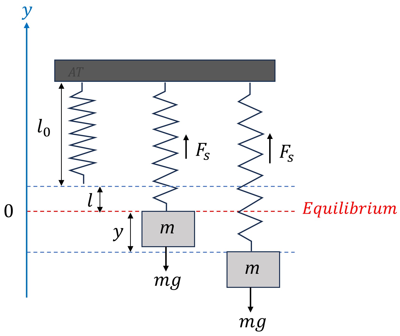
To derive the equation governing the motion of a spring-mass-damper system, we apply Newton’s second law of motion, which relates the net force acting on the mass to its acceleration. The primary forces acting on the mass in a spring-mass system include:

Force due to gravity $F_g=mg$ acting downward.
Restorative Force of the spring $F_s=-k(l+y)$ , where $k$ is the spring constant. This force is governed by Hooke’s law and is typically proportional to the displacement from the spring’s natural length ( $l_0$ ) and opposite in direction.
Damping Force $F_d=-cy'$ , where $c$ is the damping coefficient. If present, the damping force is proportional to the velocity of the mass and acting in the opposite direction of motion.
External Force $F(t)$ . It includes any external force acting on the system, which might be periodic or random, leading to forced vibrations.

According to Newton’s second law,

$ma=sumF$

Substituting all the forces and writing acceleration as the second derivative of displacement yields

$my''=F_g+F_s+F_d+F(t)$

$my''=mg-k(l+y)-cy'+F(t)$

$my''+cy'+ky=mg-kl+F(t)$

At equilibrium, the sum of all forces acting on the mass equals zero. Therefore,

$sumF=0$

$F_g+F_s=0$

$mg-kl=0$

$mg=kl$

Simplify the equation by incorporating $mg=kl$ to focus on deviations from equilibrium, leading to the standard form of the vibration equation.

$my''+cy'+ky=F(t)$ (3.8.1)

Here, $y$ is the displacement from the equilibrium position, $y'$ is the velocity, $y''$ is the acceleration, and $F(t)$ represents any external force applied to the system. We usually solve this equation along with the initial conditions for initial displacement from the equilibrium position: $y(0)=y_0$ and initial velocity: $yprime (0)=y'_0$ .

Depending on which forces act on the system, there are several special cases:

Free Undamped Vibration ( $c=0, \ F(t)=0$ ): The simplest form of vibration occurs when there is no damping and no external force. The system oscillates at its natural frequency, determined by the mass and spring constant.
Free Damped Vibration ( $cgt0,\ F(t)=0$ ): When damping is present but there is no external force, the system experiences damped vibrations leading to a gradual decrease in oscillation amplitude over time. The nature of the damping (underdamped, critically damped, or overdamped) depends on the values of $m$ , $c$ , and $k$ .
Forced Undamped Vibration ( $c=0, \ F(t)ne0$ ): When an external force acts on the system, the system experiences forced vibrations. If the frequency of the external force is close to the system’s natural frequency, resonance can occur, leading to large amplitude oscillations.
Forced Damped Vibration ( $cgt0, \ F(t)ne0$ ): This is the most general case, combining the effects of damping and external forcing, leading to complex oscillatory behavior.

D. Free Undamped Vibration

The simplest form of vibration occurs when there is no damping ( $F_d=0$ ) and no external force ( $F(t)=0$ ). In such cases, Equation 3.8.1 reduces to

$my''+ky=0$ (3.8.2)

This equation is a homogeneous second-order linear differential equation. By solving the characteristic equation $mr^2+k=0$ , we find that the roots are complex conjugates given by

$r=+-isqrt(k/m)$

The term $sqrt(k/m)$ is known as the natural frequency of the system, denoted by $omega_0$ . Therefore the solution to the equation is expressed as

$y(t)=c_1cos(omega_0t)+c_2sin(omega_0t)$ (3.8.3)

It is often convenient to represent the displacement in the amplitude-phase form with a single trigonometric function

$y(t)=Rcos(omega_0t-phi)$ (3.8.4)

Here $R$ is the amplitude of oscillation, given by $R=sqrt(c_1^2+c_2^2)$ and $phi$ is the phase angle, which can be determined from the initial conditions of the system. The phase angle $phi$ is typically chosen to satisfy $-pilephiltpi$ for uniqueness and is related to $c_1$ and $c_2$ .

$phi=tan^-1(c_2/c_1),$

$cos(phi)=c_1/R=c_1/(sqrt(c_1^2+c_2^2))$ and $sin(phi)=c_2/R=c_2/(sqrt(c_1^2+c_2^2))$

The motion described by Equation 3.8.4 is known as simple harmonic motion, characterized by its sinusoidal nature and constant frequency. The period of the motion is $T=(2pi)/(omega_0)$ , representing the time it takes to complete one full cycle.

Considerations for Units and Phase Angle

Units: When working with the acceleration due to gravity or any other physical quantity, it is important to use consistent units throughout the calculation. In the metric system, $g$ is typically given as $9.81\ "m"//"s"^2$ , and lengths should be in meters with mass in kilograms. In the Imperial system, $g$ is about $32 \ "ft"//"s"^2$ , with lengths in feet and mass in slugs.
Phase Angle Uniqueness: There are infinitely many phase angles that satisfy the trigonometric equations due to their periodic nature. However, selecting $phi$ in the interval $[-pi ,pi)$ ensures a unique solution within one complete cycle. The signs of $c_1$ and $c_2$ determine the quadrant in which $phi$ lies.
- if $c_1,c_2gt0$ , $phi$ is in the first quadrant
- If $c_1lt0,\ c_2gt0$ , $phi$ is in the second quadrant.
- if $c_1,\ c_2lt0$ , $phi$ is in the third quadrant.
- If $c_1gt0, \ c_2lt0$ , $phi$ is in the fourth quadrant.

Example 3.8.1: Simple Harmonic Motion

A 150 cm long vertical spring hangs from a fixed ceiling. A 2-kg object is attached to the lower end of the spring, and the length of the spring becomes 155 cm where the object is in equilibrium. The object is then pulled down an additional 3 cm and released with an initial upward velocity of 20 cm/s. Assuming no damping and no external forces other than gravity are acting on the system:

a) Find the displacement of the object as a function of time.

b) Determine the natural frequency, period, amplitude, and phase angle of the motion.

c) Rewrite the equation of motion in the amplitude-phase form $y(t) = R cos(omega_0 t - phi)$ .

Express your answers in the cgs unit where $g=980\ "cm"//"s"^2$ .

Show/Hide Solution

Given information:

Natural length of the spring: $l_0=150 \ "cm"$
Length at equilibrium with a 2-kg object attached: $l_0+l=155 "cm"$
Mass of the object: $m=2 \ "kg"=2000 \ "g"$
Initial displacement (downward): $y_0(0)=-3 \ "cm"$
Initial velocity (upward): $y'_0(0)=20\ "cm"//"s"$

Calculating the spring constant

At equilibrium, the forces acting on the object are balanced, meaning $F_g=F_s$ . This allows us to determine the spring constant $k$ .

\ k/m=g/(l)" title="mg=k(l) ->\ k/m=g/(l)" class="asciimath mathjax">

$k/m=980/5 =196$

$k=196(2000)=392,000\ "dyne/cm"$

Calculating the natural frequency:

The natural frequency is

$omega_0=sqrt(k/m) =sqrt(196)=14$

It is important to note that to find $omega_0$ , we require the ratio of $k$ and $m$ rather than their individual values.

Finding the general solution:

Given there is no damping force and an external force, the initial value problem is

$2y''+392y=0,$ $y_0(0)=-3,$ $y'_0(0)=20$

The general solution to this equation is given by Equation 3.8.3.

$y(t)=c_1cos(14t)+c_2sin(14t)$

Applying the initial conditions:

$y_0(0)=-3$

$c_1cos(0)+c_2sin(0)=-3$

$c_1=-3$

$y'(t)=-14c_1sin(14t)+14c_2cos(14t)$

$y'_0(0)=20$

$-14c_1sin(0)+14c_2cos(0)=20$

$14c_2=20$

$c_2=10/7$

The equation of the object displacement is then

$y(t)=-3cos(14t)+10/7sin(14t)$

Natural frequency: $omega_0=14 \ "rad"//"s"$

Period: $T=(2pi)/(omega_0)=pi/7 \ "s"$

Amplitude $R$ is given by

$R=sqrt(c_1^2+c_2^2)$

$R=sqrt((-3)^2+(10/7)^2)=1/7sqrt(541)$

Phase angle:

The reference phase angle is determined by

$phi=tan^-1(|c_2/c_1|)$

$phi_R=tan^-1(|(10//7)/-3|)~~0.444 \ "rad"$

Since $c_1lt0$ ( $cos(phi)lt0$ ) and $c_2gt0$ ( $sin(phi)gt0$ ), $phi$ should be in the second quadrant. Therefore,

$phi=pi-phi_R ~~ 2.697\ "rad"$ .

c) The equation of motion can be written as

$y(t) = R cos(omega_0 t - phi)$

$y(t) = 1/7sqrt(541) cos(14 t - 2.697)$

The graph of the displacement is shown for the first 7 seconds.

Graph of y(t) is a sinusoidal curve with amplitude of 1/7sqrt(541) and phase shift of 2.697.

Try an Example

One or more interactive elements has been excluded from this version of the text. You can view them online here: https://ecampusontario.pressbooks.pub/diffeq/?p=182

E. Free Damped Vibration

In free, damped vibration, there is no external force ( $F(t)=0$ ). As such, Equation 3.8.1 simplifies to a homogeneous second-order linear differential equation.

$my''+cy'+ky=0$ (3.8.5)

This equation is a homogeneous second-order linear differential equation. By solving the characteristic equation $mr^2+cr+k=0$ using the quadratic formula, we find the roots

$r_(1,2)=(-c+-sqrt(c^2-4mk))/(2m)$

Depending on the discriminant $c^2-4mk$ , we encounter three types of motion:

1. Critically damped ( $c^2-4mk=0$ )

In this case, there is a repeated root $r=-c/(2m)$ , and thus the general solution to Equation 3.8.5 becomes

$y(t)=c_1e^(-c/(2m)t)+c_2te^(-c/(2m)t)$ (3.8.6)

The motion in this case is said to be critically damped as the damping is just enough to prevent oscillation. This level of damping is achieved when the damping coefficient $c$ .

$c^2-4mk=0$

$c^2=4mk$

$c=2sqrt(mk)$

$2sqrt(mk)$ is called the critical damping coefficient and is denoted by $C_(cr)$ .

$c_(cr)=2sqrt(mk)$

It is important to note that as time progresses ( $trarroo$ ), the displacement $y(t)$ approaches zero, indicating that the system smoothly and quickly settles to its equilibrium position without oscillation and overshooting the equilibrium position similar to how shock absorbers work in automotive suspension systems.

2. Overdamped ( $c^2-4mkgt0$ )

In this case, there are two real distinct roots $r_(1,2)=(-c+-sqrt(c^2-4mk))/(2m)$ , where both roots are negative. The general solution to Equation 3.8.5 becomes

$y(t)=c_1e^(r_1t)+c_2e^(r_2t)$ (3.8.7)

Given both $r_1$ and $r_2$ are negative, as time progresses ( $trarroo$ ), the displacement $y(t)$ approaches zero and the system gradually returns to equilibrium without oscillating. Overdamped conditions arise when $cgtc_(cr)$ , typically desired in systems where overshooting the equilibrium position could be harmful or undesirable, like in heavy machinery. Overdamped systems return to equilibrium slower than critically damped systems. This slower response is due to the higher damping force applied, which prevents oscillation but also resists motion, causing a sluggish return.

3. Underdamped ( $c^2-4mklt0$ )

In this case, the roots of the characteristic equation are complex conjugates given by

$r_(1,2)=-c/(2m)+-(sqrt(4mk-c^2))/(2m)i=-c/(2m)+-omega_1i$

Thus the solution to the differential Equation 3.8.5 is

$y(t)=e^(-c/(2m)t)(c_1cos(omega_1t)+c_2sin(omega_1t))$ (3.8.8)

The term $omega_1=(sqrt(4mk-c^2))/(2m)$ is related to the frequency of oscillation. Similar to the harmonic motion, we can derive the amplitude-phase form of the equation of motion.

$y(t)=Re^(-c/(2m)t)cos(omega_1t-phi)$ (3.8.9)

Here again

$R=sqrt(c_1^2+c_2^2)$ , $cos(phi)=(c_1)/R$ , and $sin(phi)=(c_2)/R$

An underdamped system is characterized by a damping coefficient $cltc_(cr)$ . In this scenario, the damping is insufficient to halt oscillations, causing the system to exhibit oscillatory behavior around the equilibrium position. The amplitude of these oscillations diminishes over time, represented by the time-varying term $Re^(-c/(2m)t)$ . As the exponent $-c/(2m)$ is always negative, the displacement $y(t)$ gradually approaches zero as time progresses ( $trarroo$ ). This results in a bouncy system response to any disturbances.

Such behavior is often preferred in various applications. In musical instruments, for example, the underdamped vibrations of strings or membranes contribute to a sustained, resonant sound. Similarly, seismic dampers in buildings employ a controlled underdamped response to safely dissipate energy from earthquakes, allowing structures to sway and reduce stress without collapsing.

Example 3.8.2: Critically Damped Motion

A 1-kg mass is attached to a string with a stiffness of 64 N/m and a dashpot with a damping constant 16 N.s/m. The object is compressed 20 cm above its equilibrium and released with an initial upward velocity of 2 m/s. Find the displacement of the object as a function of time.

Show/Hide Solution

Given information:

Mass of the object: $m=1 \ "kg"$
Damping constant: $c=16 \ "N"*"s"//"m"$
Spring constant: $k=64 \ "N/m"$
Initial displacement (upward): $y_0(0)=20 \ "cm"=$ $0.2 \ "m"$
Initial velocity (upward): $y'_0(0)=2\ "m"//"s"$

The initial value problem for this system is

$y''+16y'+64y=0,$ $y_0(0)=0.2,$ $y'_0(0)=2$

Before solving the IVP, we can calculate the critical damping coefficient to determine the type of damping.

$c_(cr)=2sqrt(mk)$

$c_(cr)=2sqrt(1(64))=16$

The damping coefficient equals the critical damping coefficient ( $c=c_(cr)=16$ ), and therefore, the system is critically damped.

Finding the general solution:

The general solution for a critically damped system is given by Equation 3.8.6.

$y(t)=c_1e^(-c/(2m)t)+c_2te^(-c/(2m)t)$

$y(t)=c_1e^(-8t)+c_2te^(-8)$

Applying the initial conditions:

$y_0(0)=0.2$

$c_1e^(0)+0=0.2$

$c_1=0.2$

$y'(t)=-8c_1e^(-8t)+c_2e^(-8t)(1-8t)$

$y'_0(0)=2$

$-8c_1e^(0)+c_2e^0(1)=2$

$-8(0.2)+c_2=2$

$c_2=3.6$

The equation of the object’s displacement is then

$y(t)=0.2e^(-8t)+3.6te^(-8t)$

The graph of the displacement is shown for the first 3 seconds. As expected, the system smoothly and quickly returns to its equilibrium position without oscillation.

Graph of y(t) starts at y-intercept of 0.2, peaks at about t = 0.1 and sharply decreases to close to x-axis.

Try an Example

One or more interactive elements has been excluded from this version of the text. You can view them online here: https://ecampusontario.pressbooks.pub/diffeq/?p=182

Example 3.8.3: Overdamped Motion

Find the displacement of the object in Example 3.8.2, if the spring is now attached to a dashpot with a damping constant 34 N.s/m.

Show/Hide Solution

Given information:

Mass of the object: $m=1 \ "kg"$
Damping constant: $c=34 \ "N"*"s"//"m"$
Spring constant: $k=64 \ "N/m"$
Initial displacement (upward): $y_0(0)=20 \ "cm"=$ $0.2 \ "m"$
Initial velocity (upward): $y'_0(0)=2\ "m"//"s"$

The initial value problem for this system is

$y''+34y'+64y=0,$ $y_0(0)=0.2,$ $y'_0(0)=2$

In the previous example, we determined the critical damping coefficient to be $c_(cr)=16$ . In the current system, the damping coefficient is greater than this critical value (c_(cr)=16" title="c>c_(cr)=16" class="asciimath mathjax">), and therefore, the system is overdamped.

Finding the general solution:

The characteristic equation for the differential equation has two distinct real roots.

$r_(1,2)=(-34+-sqrt(34^2-4(1)(64)))/(2(1))$

$r_1=-2,$ $r_2=-32$

The general solution to an overdamped system is given by Equation 3.8.7.

$y(t)=c_1e^(r_1t)+c_2e^(r_2t)$

$y(t)=c_1e^(-2t)+c_2e^(-32t)$

Applying the initial conditions:

$y_0(0)=0.2$

$c_1e^(0)+c_2e^0=0.2$

$c_1+c_2=0.2$

$y'(t)=-2c_1e^(-2t)-32c_2e^(-32t)$

$y'_0(0)=2$

$-2c_1e^(0)-32c_2e^0=2$

$-2c_1-32c_2=2$

Solving the system for constants $c_1$ and $c_2$ yields

$c_1=0.28, \ c_2=-0.08$

The equation of the object’s displacement is then

$y(t)=0.28e^(-2t)-0.08e^(-32t)$

The below graph displays the displacement for the first 3 seconds. It confirms that the system gradually returns to its equilibrium position smoothly and without any oscillation. When compared to the critically damped system in Example 3.8.2, this overdamped system takes a longer time to settle down. This slower behavior underscores that the increased damping force in the overdamped system delays the return to equilibrium.

Graph of the displacement y(t) for the first 3 seconds. It starts from the y-intercept of 0.2, peaks at about t=0.1s and decreases smoothly to approach y=0.

Try an Example

One or more interactive elements has been excluded from this version of the text. You can view them online here: https://ecampusontario.pressbooks.pub/diffeq/?p=182

Example 3.8.4: Underdamped Motion

Find the displacement of the object in Example 3.8.2, if the spring is now attached to a dashpot with a damping constant 4 N.s/m.

Show/Hide Solution

Given information:

Mass of the object: $m=1 \ "kg"$
Damping constant: $c=4 \ "N"*"s"//"m"$
Spring constant: $k=64 \ "N/m"$
Initial displacement (upward): $y_0(0)=20 \ "cm"=$ $0.2 \ "m"$
Initial velocity (upward): $y'_0(0)=2\ "m"//"s"$

The initial value problem for this system is

$y''+4y'+64y=0,$ $y_0(0)=0.2,$ $y'_0(0)=2$

In Example 3.8.2, we determined the critical damping coefficient to be $c_(cr)=16$ . In the current system, the damping coefficient is less than this critical value ( $cltc_(cr)=16$ ), and therefore, the system is underdamped.

Finding the general solution:

The characteristic equation for the differential equation has complex conjugates.

$r_(1,2)=-4/(2(1))+-(sqrt(4(1)(64)-4^2))/(2(1))i=-2+-2sqrt(15)i$

The general solution to an underdamped system is given by Equation 3.8.8.

$y(t)=e^(-2t)(c_1cos(2sqrt(15)t)+c_2sin(2sqrt(15)t))$

Applying the initial conditions:

$y_0(0)=0.2$

$e^(0)(c_1cos(0)+c_2sin(0))=0.2$

$c_1=0.2$

$y'(t)=e^(-2t)(-2c_1cos(2sqrt(15)t)-2c_2sin(2sqrt(15)t)-$ $2sqrt(15) c_1sin(2sqrt(15)t)+2sqrt(15) c_2cos(2sqrt(15)t))$

$y'_0(0)=2$

$-2c_1+2sqrt(15)c_2=2$

$-2(0.2)+2sqrt(15)c_2=2$

$c_2=(2sqrt(15))/25$

The equation of the object’s displacement is then

$y(t)=e^(-2t)(0.2cos(2sqrt(15)t)+(2sqrt(15))/25 sin(2sqrt(15)t))$

The amplitude-phase form of the equation is

$y(t)=sqrt(85)/25e^(-2t)cos(2sqrt(15)t-0.9976)$

The graph illustrates the displacement of the system over the initial 3 seconds. This underdamped system lacks enough damping to stop oscillations, leading to a pattern of diminishing swings around the equilibrium position. These oscillations decrease in amplitude for approximately 2 seconds before the system finally settles at the equilibrium position.

Graph of y(t) starts at y-intercept of about 0.17m. It increases to y=0.28 and then decreases crossing the x-axis. This underdamped system lacks enough damping to stop oscillations, leading to a pattern of diminishing swings around the equilibrium position. These oscillations decrease in amplitude for approximately 2 seconds before the system finally settles at the equilibrium position.

Try an Example

One or more interactive elements has been excluded from this version of the text. You can view them online here: https://ecampusontario.pressbooks.pub/diffeq/?p=182

F. Forced Undamped Vibration

Forced undamped vibration occurs in systems subject to a continuous external force, typically modeled as a periodic function like $F(t)=F_0 cos(omega t)$ or $F(t)=F_0 sin(omega t)$ . These sinusoidal forces commonly arise from rotational mechanisms, alternating currents, or other cyclic phenomena. The equation of motion for such a system is expressed as

$my''+ky=F_0cos(omega t)$

The solution to the differential equation is

$y(t)=y_p (t)+y_c (t)$

Here, the solution comprises a complementary part $y_c(t)$ , representing the free, undamped vibration response, and a particular part $y_p(t)$ , the steady-state response to the forcing function. The complementary solution, dictated by the system’s natural frequency $omega_0=k/m$ , is given by Equation 3.8.3:

$y_c(t)=c_1cos(omega_0t)+c_2sin(omega_0t)$

To determine the particular solution, we typically use methods like undetermined coefficients or variation of parameters. As we seek the particular solution, depending on the driving frequency omega, we consider two cases:

1. Non-Resonant ( $omega!=omega_0$ ): When the driving frequency is different from the natural frequency, the particular solution is in the form

$Y_p(t)=Acos(omegat)+Bsin(omegat).$

To find the specific values of the coefficients A and B, we use the method of undetermined coefficients. After determining these coefficients, the particular solution can be expressed as

$y_p=F_0/(m(omega_0^2-omega^2))cos(omega t),$

and the general solution is

$y(t)=F_0/(m(omega_0^2-omega^2))cos(omega t)+$ $c_1cos(omega_0t)+c_2sin(omega_0t)$ (3.8.10)

The displacement function consists of sine and cosine components with bounded amplitude.

2. Resonant ( $omega=omega_0$ ): When the driving frequency is equal to the natural frequency, the particular solution is in the form

$Y_p(t)=t(Acos(omegat)+Bsin(omegat))$

using the method of undetermined coefficients and after determining the coefficients, the particular solution can be expressed as

$y_p=F_0/(2m omega_0)t sin(omega_0 t)$

The general solution is then

$y(t)=F_0/(2m omega_0)t sin(omega_0 t)+$ $c_1cos(omega_0t)+c_2sin(omega_0t)$ (3.8.11)

In this case, the particular solution includes a time factor $t$ , indicating the unbounded increase in amplitude. This phenomenon, known as resonance, significantly increases oscillation amplitude and poses potential risks, including mechanical failure from excessive oscillations.

The amplitude of oscillation in forced vibration is sensitive to the relationship between the driving frequency and the natural frequency of the system. As the driving frequency approaches the natural frequency, the amplitude increases, peaking at resonance. This sensitivity is a key factor in designing structures and systems to ensure their natural frequencies are not aligned with frequencies of common environmental forces, like wind or traffic. Such alignment could trigger resonance, risking structural integrity.

On the other hand, there are specific applications where inducing resonance is advantageous, for instance, in mechanical filters and sensors, where resonance can enhance sensitivity or signal strength.

Example 3.8.5: Forced Undamped Vibration

A 32 lb object is suspended from a spring, stretching it by 6 inches to reach equilibrium. This undamped system is subjected to an external force $F(t) = 2cos(8t)$ , and it experiences resonance. Initially, the object is displaced 3 inches below the equilibrium position and is given an upward velocity of 1 ft/s. Determine the object’s displacement under these conditions.

Show/Hide Solution

Given information:

Mass of the object: $W=32 \ "lb"$
The spring displacement at equilibrium: $l= 6 \ "in"=1/2 \ "ft"$
External force: $F(t) = 2 cos(8t)$
Initial displacement (downward): $y_0(0)=-3\ "in"=$ $-0.25 \ "ft"$
Initial velocity (upward): $y'_0(0)=1\ "ft"//"s"$

Calculating the spring constant

In the British system, weight is typically measured in pounds. To find the spring constant, we first convert weight to mass using the formula

$W=mg$

$m=W/g=32/32=1 \ "slug"$

At equilibrium $F_g=F_s$ . This relationship allows us to calculate the spring constant $k$ .

\ k=(mg)/( l)" title="mg=k( l) ->\ k=(mg)/( l)" class="asciimath mathjax">

$k=64\ "lbf/ft"$

Calculating the natural frequency:

The natural frequency is

$omega_0=sqrt(k/m) =sqrt(64)=8$

Alternatively, if the system resonates at a driving frequency of $omega=8$ (from $F(t) = 2 cos(8t)$ ), this resonance frequency should match the natural frequency of the system, reaffirming that $omega_0=8$ .

Finding the general solution:

The initial value problem for this system is

$y''+64y=2cos(8t),$ $y_0(0)=-0.25,$ $y'_0(0)=1$

The general solution for a system undergoing resonance is given by Equation 3.8.11.

$y(t)=2/(2(1)(8))t sin(8 t)+c_1cos(8t)+c_2sin(8t)$

$y(t)=1/8t sin(8 t)+c_1cos(8t)+c_2sin(8t)$

Applying the initial conditions:

" title="y_0(0)=-0.25 \ ->" class="asciimath mathjax"> $c_1=-0.25=-1/4$

" title="y'_0(0)=1\ ->" class="asciimath mathjax"> $c_2=0.125=1/8$

The equation of the object’s displacement is then

$y(t)=1/8t sin(8 t)-1/4cos(8t)+1/8sin(8t)$

We can write the complementary solution in the amplitude-phase form, combining the last two terms.

$y(t)=1/8tsin(8t)+sqrt(5)/8cos(8t-2.6779)$

The graph shows how the system’s displacement changes during the first 10 seconds. Since the particular solution includes a time factor (t), the displacement’s amplitude tends to become infinitely large as time progresses towards infinity. However, in reality, most systems experience some damping. Even a small amount of damping can significantly affect the system’s amplitude and behavior, especially around resonance frequencies, preventing the unlimited growth in amplitude predicted by ideal models.

Graph of y(t) starts at the y-intercept of about y=-0.27. It oscillates with an amplitude that becomes infinitely large as time approaches infinity.

Try an Example

One or more interactive elements has been excluded from this version of the text. You can view them online here: https://ecampusontario.pressbooks.pub/diffeq/?p=182

G. Forced Damped Vibration

This is the most general case, combining the effects of damping and external forcing. The motion of such a system is governed by

$my''+cy'+ky=F_0cos(omega t)$

The solution to the differential equation is the sum of complementary and particular solutions.

$y(t)=y_p (t)+y_c (t)$

The complementary solution is the solution to the free, damped behavior, while the particular solution is found using the method of undetermined coefficients or variation of parameters.

Based on our understanding of free-damped vibrations, we know that as time progresses toward infinity, the complementary solution approaches zero. Consequently, the system’s displacement increasingly reflects the behavior of the particular solution. Therefore, in vibrational analysis, the complementary solution is commonly referred to as the transient solution, reflecting the initial response, while the particular solution is known as the steady-state solution, indicating the ongoing response to the external force.

Example 3.8.6: Forced Damped Vibration

Find the displacement of the object in Example 3.8.5, if the system is now attached to a dashpot with a damping constant 34 lb.s/ft.

Show/Hide Solution

Given information:

Mass of the object: $W=32 \ "lb"$
The spring displacement at equilibrium: $l= 6 \ "in"=1/2 \ "ft"$
Damping constant: $c=20\ "lb.s/ft"$
External force: $F(t) = 2 cos(8t)$
Initial displacement (downward): $y_0(0)=-3\ "in"=$ $-0.25 \ "ft"$
Initial velocity (upward): $y'_0(0)=1\ "ft"//"s"$

In the previous example, we determined the spring constant: $k=64\ "lbf/ft"$ . The initial value problem for this system is

$y''+20y'+64y=2cos(8t),$ $y_0(0)=-0.25,$ $y'_0(0)=1$

Given the characteristic equation has distinct real roots $r_1=-4$ and $r_2=-16$ , the complementary solution, according to Equation 3.8.7, is

$y_c(t)=c_1e^(-4t)+c_2e^(-16t)$

Finding the particular solution:

To find the particular solution, we use undetermined coefficients. Given the forcing cosine function, we guess the form of the particular solution to be

$Y_p=Acos(8t)+Bsin(8t)$

The derivatives are

$Y'_p=-8Asin(8t)+8Bcos(8t)$

$Y''_p=-64Acos(8t)-64Bsin(8t)$

Substituting $Y_p$ and its derivatives into the differential equation yields

$-64Acos(8t)-64Bsin(8t)+20(-8Asin(8t)+8Bcos(8t))$ $+64(Acos(8t)+Bsin(8t))=2cos(8t)$

Simplifying it gives

$160Bcos(8t)-160Asin(8t)=2cos(8t)$

By matching coefficients of sine and cosine terms, we get

\ B=1/80" title="160B=2\ ->\ B=1/80" class="asciimath mathjax">

\ A=0" title="-160A=0\ ->\ A=0" class="asciimath mathjax">

Therefore, the particular solution is

$y_p=1/80sin(8t)$

Combining the particular and complementary solutions gives the general solution

$y(t)=1/80sin(8t)+$ $c_1e^(-4t)+c_2e^(-16t)$

Applying the initial conditions:

" title="y_0(0)=-0.25 \ ->" class="asciimath mathjax"> $c_1+c_2=-1/4$

" title="y'_0(0)=1\ ->" class="asciimath mathjax"> $-4c_1-16c_2=9/10$

Solving the system, we find the constants to be

$c_1=-31/120,\ c_2=1/120$

The equation of the object’s displacement is then

$y(t)=1/80sin(8t)-$ $31/120e^(-4t)+1/120e^(-16t)$

The graph depicts the change in the system’s displacement over the first 6 seconds. Initially, for about the first second, the displacement is primarily influenced by the complementary solution, reflecting the transient phase. After this initial period, the displacement increasingly aligns with the periodic particular solution, representing the steady-state behavior of the system.

Graph of y(t) starts at the y-intercept of y=-0.25 and increases until it crosses x-axis. It then looks like a sinusoidal curve oscillating with amplitude of 1/80.

Try an Example

One or more interactive elements has been excluded from this version of the text. You can view them online here: https://ecampusontario.pressbooks.pub/diffeq/?p=182

Section 3.8 Exercises

An object attached to a spring undergoes simple harmonic motion modeled by the differential equation
$m(d^2 y)/(dt^2) + ky = 0$

where $y(t)$ is the displacement of the mass (relative to equilibrium) at time $t$ , $m$ is the mass of the object, and $k$ is the spring constant. A mass of $15\ "kg"$ stretches the spring $0.25\ "m"$ . a) Use this information to find the spring constant. (Use $g = 9.8\ "m"//"s"^2$ ). b) The previous mass is detached from the spring and a mass of $2\ "kg"$ is attached. This mass is displaced $0.1\ "m"$ above equilibrium (above is positive and below is negative) and then launched with an initial velocity of $2\ "m"//"s"$ . Write the equation of motion in the form $y(t) = c_1 cos(omega t) + c_2 sin(omega t)$ . Do not leave unknown constants in your equation.

Show/Hide Answer

a) $k=588$ N/m

b) $y(t)=1/10cos(7sqrt(6)t)+2/(7sqrt(6))sin(7sqrt(6)t)$
A $13\ "kg"$ object is attached to a spring with spring constant $9\ "kg"//"s"^2$ . It is also attached to a dashpot with damping constant $9\ "kg"//"s"$ . The object is initially displaced $5\ m$ above equilibrium and released. a) Find its displacement for 0" title="t > 0" class="asciimath mathjax">. b) Describe the motion.

Show/Hide Answer

a) $y(t)=e^(-9/26t)(5cos(sqrt(387)/(26)t)+45/sqrt(387)sin(sqrt(387)/(26)t))$

b) Free underdamped vibration
A $16\ "kg"$ object is attached to a spring with spring constant $64$ $"kg"//"s"^2$ . It is also attached to a dashpot with damping constant $c = 64$ $"kg/s"$ . The object is pulled down $0.1 \ m$ and released with an initial upward velocity of $4 \ "m/s"$ . Find the displacement of the object. Assume displacement and velocity are positive upward.

Show/Hide Answer

$y(t)=-0.1 e^(-2t)+3.8te^(-2t)$

3.9 Application: RLC Electrical Circuits

In Section 2.5F, we explored first-order differential equations for electrical circuits consisting of a voltage source with either a resistor and inductor (RL) or a resistor and capacitor (RC). Now, equipped with the knowledge of solving second-order differential equations, we are ready to delve into the analysis of more complex RLC circuits, which incorporate a resistor, inductor, and capacitor.

Previously, we established that:

Ohm’s law dictates that the voltage drop $E_R$ across a resistor is proportional to the current I flowing through it, expressed as $E_R=RI$ , where $R$ is the resistance.
Faraday’s law, complemented by Lenz’s law, describes that the voltage drop $E_L$ across an inductor is proportional to the rate of change of current, given as $E_L=L(dI)/(dt)$ , where $L$ is the inductance.
The voltage drop $E_C$ across a capacitor is proportional to the electric charge $q$ stored on it, represented as $E_C=1/Cq$ , with $C$ being the capacitance

Schematic of an RLC circuit consisting of a resistor, a capacitor, and an inductor in a series circuit

Figure 3.9.1 Schematic of an RLC series circuit

With these foundations, consider $E(t)$ as the external voltage supplied to the RLC series circuit in Fig. 3.9.1. By applying Kirchhoff’s voltage law, we have

$E_L+E_R+E_c=E(t)$

Substituting $E_R=RI$ , $E_L=L (dI)/dt$ , and $E_C=1/Cq$ into this equation yields

$L (dI)/dt+RI+1/Cq=E(t)$ (3.9.1)

Differentiating this equation with respect to time and substituting $I=(dq)/dt$ transform it into a second-order differential equation.

$L(d^2I)/(dt^2)+R (dI)/dt+1/CI=(dE)/dt$ (3.9.2)

Alternatively, Equation 3.9.1 can be expressed in terms of charge $q(t)$ .

$L (d^2q)/(dt^2)+R(dq)/(dt)+1/Cq=E(t)$ (3.9.3)

Given $E(t)$ and an initial condition, such as initial current $I(0)$ and initial charge $q(0)$ , we can solve the equation for $I(t)$ using techniques discussed in previous sections, such as the method of undetermined coefficients. Once $I(t)$ is determined, the voltage across different components of the circuit can be calculated.

Example 3.9.1: RLC Series Circuit

Consider an RLC series circuit with a resistor of $0.06\ Omega$ and an inductor of $0.01\ "H"$ , and a capacitor of $50/89\ "F"$ powered by a voltage source $E(t)=0.1sin(10t)\ "V"$ . Initially, the current and charge on the capacitor are zero. Determine the current in the circuit as a function of time.

Show/Hide Solution

Given information:

Resistor: $R=0.06\ Omega$
Inductor: $L=0.01 \ "H"$
Capacitor: $C=50/89\ "F"$
Voltage source: $E(t)=0.1sin(10t)\ "V"$
Initial current on capacitor: $I(0)=0 \ "A"$
Initial charge on capacitor: $q(0)=I'(0)=0 \ C$

The differential equation for an RLC series circuit is given by Equation 3.9.1.

$L(d^2I)/(dt^2)+R (dI)/dt+1/CI=(dE)/dt$

The initial value problem is then

$0.01(d^2I)/(dt^2)+0.06 (dI)/dt+89/50I=cos(10t),$ $I(0)=0, \ I'(0)=0$

Multiplying the equation by 100, we get

$(d^2I)/(dt^2)+6 (dI)/dt+178I=100cos(10t),$ $I(0)=0, \ I'(0)=0$

Given the characteristic equation has complex conjugates $r_(1,2)=-3+-13i$ , the complementary solution is

$I_c(t)=e^(-3t)(c_1cos(13t)+c_2sin(13t))$

Finding the particular solution:

To find the particular solution, we use undetermined coefficients. Given the forcing cosine function, we guess the form of the particular solution to be

$I_p=Acos(10t)+Bsin(10t)$

The derivatives are

$I'_p=-10Asin(10t)+10Bcos(10t)$

$I''_p=-100Acos(10t)-100Bsin(10t)$

Substituting $I_p$ and its derivatives into the differential equation yields

$-100Acos(10t)-100Bsin(10t) +6(-10Asin(10t)+10Bcos(10t) )$ $+178(Acos(10t)+Bsin(10t))=$ $100cos(10t)$

Simplifying gives

$(78A+60B)cos(10t)+(-60A+78B)sin(10t)=100cos(10t)$

By matching coefficients of sine and cosine terms and solving the system of two equations in unknowns $A$ and $B$ , we get

$A=650/807,\ B=500/807$

Therefore, the particular solution is

$I_p=650/807cos(10t)+500/807sin(10t)$

Combining the particular and complementary solutions gives the general solution

$I(t)=650/807cos(10t)+500/807sin(10t) +$ $e^(-3t)(c_1cos(13t)+c_2sin(13t))$

Applying the initial conditions:

" title="I_0(0)=0 \ ->" class="asciimath mathjax"> $c_1=-650/807$

" title="I'_0(0)=0\ ->" class="asciimath mathjax"> $c_2=-6950/10491$

The equation of the object’s displacement is then

$I(t)=650/807cos(10t)+500/807sin(10t) +$ $e^(-3t)(-650/807 cos(13t)-6950/10491 sin(13t))$

As with forced mechanical vibration scenarios, the current in an RLC circuit is composed of two distinct parts: the transient current, represented by the complementary solution that diminishes to zero as time progresses to infinity, and the steady-state current, described by the particular solution which is sinusoidal and persists over time.

Try an Example

One or more interactive elements has been excluded from this version of the text. You can view them online here: https://ecampusontario.pressbooks.pub/diffeq/?p=184

Section 3.9 Exercises

Consider an RLC circuit with a $17/50\Omega$ resistor, a $1/100\H$ inductor, and a $100/93\F$ capacitor driven by the voltage $E(t) = 0.06sin(3t)V$ . a) Write the differential equation associated with this circuit in terms of current $I$ . b) If the initial charge and initial current on the capacitor are both zero, find the current $I$ and the voltages across the resistor $E_R$ in terms of time $t$ .

Show/Hide Answer

a) $I''+34I'+93I = 18cos(3t)$

b) $I(t)=0.0205 e^(-31t)-0.1071 e^(-3t)+$ $0.1052sin(3t)+0.08660cos(3t)$

c) $E_R(t)=0.34(0.0205 e^(-31t)-0.1071 e^(-3t)+$ $0.1052sin(3t)+0.08660cos(3t) )$
Consider an RLC circuit with a $1/50\Omega$ resistor, a $1/100\H$ inductor, and a $50/61\F$ capacitor driven by the voltage $E(t) = 0.09t^2\ V$ . a) Write the differential equation associated with this circuit in terms of current $I$ . b) If the initial charge and initial current on the capacitor are both zero, find the current $I$ .

Show/Hide Answer

a) $I''+2I'+122I = 18t$

b) $I(t)=e^(-t)(9/3721cos(11t)-540/40931sin(11t))+9/61t-9/3721$

Laplace Transform

Chapter Outline

This chapter focuses on the Laplace Transform, an integral operator widely used to simplify the solution of differential equations by transforming them into algebraic equations in a different domain.

4.1 Definitions: This section introduces the concept and integral operator of the Laplace Transform.

4.2 Properties of Laplace Transform: This section discusses key properties of the Laplace Transform, essential for efficient function transformation and manipulation.

4.3 Inverse Laplace Transform: This section covers the process of converting functions back from the Laplace domain to the original domain, known as the inverse Laplace Transform.

4.4 Solving Initial Value Problems: This section demonstrates the application of the Laplace Transform and its inverse in solving initial value problems (IVP).

4.5 Laplace Transform of Piecewise Functions: This section explores the application of the Laplace Transform to piecewise continuous functions, using tools like the Heaviside (Unit Step) function.

4.6 Initial Value Problems with Piecewise Forcing Functions: This section discusses solving IVPs for second-order differential equations with constant coefficients and piecewise continuous forcing functions.

4.7 Impulse and Dirac Delta Function: This section introduces the Dirac Delta function and its application in solving differential equations with impulse forcing functions, which are characterized by high magnitudes over very short intervals.

4.8 Table of Laplace Transform: This section provides a table summarizing the Laplace Transform and some of its properties for quick reference.

Pioneers of Progress

Oliver Heaviside (1850-1925). Attribution: IET Archive, Public domain, via Wikimedia Commons

Oliver Heaviside, born in 1850 in Camden Town, London, was a self-taught electrical engineer, mathematician, and physicist whose unconventional approach to academia did not hinder his profound impact on the field. Largely self-educated due to financial constraints, Heaviside pursued his interest in electromagnetic theory, making substantial contributions that were both innovative and contentious at the time. His most significant achievement was the development of operational calculus, a powerful tool in the application of differential equations to physical problems, particularly in the field of electrical engineering. Heaviside’s methods simplified Maxwell’s complex equations of electromagnetism, making them more accessible and practically applicable, a feat that had a lasting impact on telecommunications and electrical engineering. Despite facing criticism and limited recognition during his lifetime, Heaviside’s work was later acknowledged as groundbreaking, influencing not only the theoretical underpinnings of electrical engineering but also the practical aspects of signal transmission and circuit design. Oliver Heaviside’s story is one of perseverance and brilliance, showcasing how a relentless pursuit of knowledge can lead to discoveries that shape the world, irrespective of the conventional academic path.

4.1 Definitions

A. Introduction

In this section, we delve into an integral operator known as the Laplace Transform. This powerful tool is employed to convert initial value problems described by differential equations in one domain (e.g., t domain) into algebraic equations in another domain (s domain). Doing so facilitates a more efficient solution process, particularly for linear differential equations with constant coefficients and discontinuous or impulsive forcing terms. For instance, consider an initial value problem in the time domain

t-Domain: $y'(t)+5y(t)=f(t),$ $y(0)=10$

Applying the Laplace Transform, the differential equation is transmuted into an algebraic equation in the s domain:

s-Domain: $sY(s)-10+5Y(s)$ $=F(s)$

This algebraic representation in the s domain is often simpler to solve, and the solution can then be transformed back to the original t domain.

B. Definition

Let $f(t)$ be a function defined on $[0,oo)$ , and let $s$ be a real number. The Laplace transform of $f$ is the function $F$ defined by the integral

$F(s)=int_0^ooe^(-st)f(t)dt$ (4.1.1)

The Laplace transform of $f$ is denoted by both $F$ and $\mathcal{L}{f}$ . The functions can also be expressed as a transform pair $f(t)harrF(s)$ .

The improper integral in the definition 4.1.1 is more precisely defined as

$int_0^ooe^(-st)f(t)dt$ oo)int_0^Te^(-st)f(t)dt" title=":=lim_(T->oo)int_0^Te^(-st)f(t)dt" class="asciimath mathjax">

The integral converges, meaning it results in a finite number when this limit exists and is finite.

Example 4.1.1: Laplace Transform of Constant Function Using Definition

Find the Laplace transform of the constant function $f(t)=2$ .

Show/Hide Solution

Substituting $f(t)=1$ into integral 4.1.1 of the definition of the Laplace transform, we obtain

$F(s)=int_0^ooe^(-st)(2)dt$ oo)int_0^Te^(-st)(2)dt" title="=lim_(T->oo)int_0^Te^(-st)(2)dt" class="asciimath mathjax">

oo)[(-2e^(-st))/s]_0^T" title="=lim_(T->oo)[(-2e^(-st))/s]_0^T" class="asciimath mathjax"> oo)[2/s-e^(-sT)/s]" title="=lim_(T->oo)[2/s-e^(-sT)/s]" class="asciimath mathjax"> 0),(oo if s<=0):}" title="= {(2/s if s>0),(oo if s<=0):}" class="asciimath mathjax">

Note that the integral diverges for $s<=0$ , so the domain of $F(s)$ is 0" title="s>0" class="asciimath mathjax"> . Since 0" title="e^(-sT)->0" class="asciimath mathjax"> when oo" title="T->oo" class="asciimath mathjax"> for a fixed $s$ , we then get

$F(s)=2/s$ for 0" title="s>0" class="asciimath mathjax"> or $2harr2/s$ as a transform pair

In general, the Laplace transform of the constant function $f(t)=C$ is $\mathcal{L}{C}=C/s$ .

Example 4.1.2: Laplace Transform of Exponential Function Using Definition

Find the Laplace transform of function $f(t)=e^(at)$ .

Show/Hide Solution

Substituting $f(t)=e^(at)$ into integral 4.1.1 of the definition of the Laplace transform, we obtain

$F(s)=int_0^ooe^(-st)(e^(at))dt$ oo)int_0^Te^(-(s-a)t)dt" title="=lim_(T->oo)int_0^Te^(-(s-a)t)dt" class="asciimath mathjax">

oo)[(-e^((s-a)t) )/(s-a)]_0^T" title="=lim_(T->oo)[(-e^((s-a)t) )/(s-a)]_0^T" class="asciimath mathjax"> oo)[1/(s-a)-e^((s-a)T)/(s-a)]" title="=lim_(T->oo)[1/(s-a)-e^((s-a)T)/(s-a)]" class="asciimath mathjax"> 0),(oo if s<=a):}" title="= {(1/(s-a) if s>0),(oo if s<=a):}" class="asciimath mathjax">

Note that the integral diverges for $s<=a$ , so the domain of $F(s)$ is a" title="s>a" class="asciimath mathjax">. Therefore,

$F(s)=1/(s-a)$ for a" title="s>a" class="asciimath mathjax"> or $e^(at)harr1/(s-a)$ as a transform pair

In practice, while the definition of the Laplace Transform involves an integral, it is rarely computed directly via integration due to the complexity and time-consuming nature of the process. Instead, we typically use precomputed tables of Laplace Transforms. These tables list common functions and their corresponding transforms, allowing for quick and accurate application of the Laplace Transform to solve differential equations and analyze systems. Table 4.1.1 includes the Laplace Transform of some common functions. A more comprehensive table can be found in Section 4.8.

Table 4.1.1: Brief Table of Laplace Transform

$f(t)$	$F(s)=$ $\mathcal{L}{f}$	Domain of $F(s)$

$C$	$C/s$	0" title="s>0" class="asciimath mathjax">
$t$	$1/s^2$	0" title="s>0" class="asciimath mathjax">
$t^n,$ $n=1,2, ...$	$(n!)/s^(n+1)$	0" title="s>0" class="asciimath mathjax">
$e^(at)$	$1/(s-a)$	a" title="s>a" class="asciimath mathjax">
$t^n\e^(at),$ $n=1,2, ...$	$(n!)/(s-a)^(n+1)$	a" title="s>a" class="asciimath mathjax">
$sin(bt)$	$b/(s^2+b^2)$	0" title="s>0" class="asciimath mathjax">
$cos(bt)$	$s/(s^2+b^2)$	0" title="s>0" class="asciimath mathjax">
$e^(at)sin(bt)$	$b/((s-a)^2+b^2)$	a" title="s>a" class="asciimath mathjax">
$e^(at)cos(bt)$	$(s-a)/((s-a)^2+b^2)$	a" title="s>a" class="asciimath mathjax">
$sinh(bt)$	$b/(s^2-b^2)$	b" title="s>b" class="asciimath mathjax">
$cosh(bt)$	$s/(s^2-b^2)$	b" title="s>b" class="asciimath mathjax">

Example 4.1.3: Laplace Transform Using Table

Use the table of Laplace Transform to determine the Laplace Transform of the following function:

a) $f(t)=sin(2t)$

b) $g(t)=cos(5t)$

Show/Hide Solution

a) From the table

$\mathcal{L}{sin(bt)}$ $=b/(s^2+b^2)$ for 0" title="s>0" class="asciimath mathjax">

Recognizing that $b=2$ , the transformation is

$\mathcal{L}{sin(2t)}$ $=2/(s^2+2^2)$ for 0" title="s> 0" class="asciimath mathjax">

b) From the table

$\mathcal{L}{cos(bt)}$ $=s/(s^2+b^2)$ for 0" title="s>0" class="asciimath mathjax">

Recognizing that $b=5$ , the transformation is

$\mathcal{L}{cos(5t)}$ $=s/(s^2+5^2)$ for 0" title="s> 0" class="asciimath mathjax">

Try an Example

One or more interactive elements has been excluded from this version of the text. You can view them online here: https://ecampusontario.pressbooks.pub/diffeq/?p=210

Section 4.1 Exercises

Find the Laplace transform, $F(s)$ , of the function $f(t) = e^(4t) , quad t gt 0$ .

Show/Hide Answer

$F(s)=1/(s-4)$
Find the Laplace Transform of, $F(s)$ , of the function $f(t) = cos(4t) , quad t gt 0$ .

Show/Hide Answer

$F(s)=s/(s^2+4^2)$
Find the Laplace transform of the function $f(t)=6 cosh(2 t)$ $, \ t gt 0$ .

Show/Hide Answer

$F(s)=(6s)/(s^2-2^2)$

4.2 Properties of Laplace Transform

Understanding the properties of the Laplace Transform is crucial as it provides tools for efficiently transforming and manipulating functions. These properties greatly simplify the analysis and solution of differential equations and complex systems.

A. Existence of the Transform

The Laplace transform exists for any function that is (1) piecewise-continuous and (2) of exponential order (i.e., does not grow faster than an exponential function). A function $f(t)$ is said to be of exponential order $a$ if there exist positive constants $M$ and $t_0$ such that $|f(t)|<=Me^(at),$ for all =t_0" title="t>=t_0" class="asciimath mathjax">. For example, $f(t)=e^(7t)cos(4t)$ is of exponential order 7, but $g(t)=e^(t^3)$ is not of exponential order.

B. Linearity of the Laplace Transform

The Laplace Transform adheres to the principle of linearity. Let $f_1$ and $f_2$ be functions whose Laplace transforms exist for s_0" title="s>s_0" class="asciimath mathjax">, and let $c_1$ and $c_2$ be constants. Then for s_0" title="s>s_0" class="asciimath mathjax">, the Laplace Transform of a linear combination of these functions is given by:

$\mathcal{L}{c_1f_1+c_2f_2}=c_1\mathcal{L}{f_1}+c_2\mathcal{L}{f_2}$

This property is useful when dealing with linear combinations of functions.

Example 4.2.1: Find Laplace Transform Using – Linearity Theorem

Use the Laplace Transform Table and the linearity property to determine

$\mathcal{L}{2e^(-3t)-6cos(4t)+9t^2}$ .

Show/Hide Solution

1. From the table

$\mathcal{L}{e^(-3t)}$ $=1/(s-(-3))=$ $1/(s+3)$ for -3" title="s> -3" class="asciimath mathjax">

$\mathcal{L}{cos(4t)}$ $=s/(s^2+4^2)=s/(s^2+16)$ for 0" title="s> 0" class="asciimath mathjax">

$\mathcal{L}{t^2}$ $=(2!)/(s^(2+1))=2/(s^3)$ for 0" title="s> 0" class="asciimath mathjax">

2. From the linearity theorem, we have

$\mathcal{L}{2e^(-3t)-6cos(4t)+9t^2 }=$ $2\mathcal{L} {e^(-3t)}-6\mathcal{L} {cos(4t)}+9\mathcal{L} { t^2}$

$=2(1/(s+3))-$ $6(s/(s^2+16) )+9(2/(s^3) )$

$=2/(s+3)-$ $(6s)/(s^2+16)+18/(s^3)$ for 0" title="s>0" class="asciimath mathjax">

Try an Example

One or more interactive elements has been excluded from this version of the text. You can view them online here: https://ecampusontario.pressbooks.pub/diffeq/?p=215

C. First Shifting (Exponential) Theorem.

If $F(s)= \mathcal{L}{f(t)}$ , then

$\mathcal{L}$ ${e^(at)f(t)}=F(s-a)$

This theorem is valuable when solving differential equations with exponential terms or in analyzing systems with exponential inputs.

Example 4.2.2: Find Laplace Transform Using – First Shifting and Linearity Theorems

Use the first shifting theorem and the linearity property to determine

$\mathcal{L}{2e^(9t)sin(7t)+8t^3 e^(-6t)}$ .

Show/Hide Solution

Using the first shifting theorem, we have

$\mathcal{L}$ ${e^(at)f(t)}=F(s-a)$

1. In $\mathcal{L}{e^(9t)sin(7t)}$ , $f(t)=sin(7t)$ and the coefficient in the exponential term’s exponent is $a=9$ .

$F(s)=\mathcal{L}{sin(7t)}$ $=7/(s^2+7^2)$ for 0" title="s>0" class="asciimath mathjax">

Shifting $F(s)$ , we substitute $s$ with $s-9.$

$\mathcal{L}{e^(9t)sin(7t)}=F(s-9)$ $=7/((s-9)^2+7^2)$ for 9" title="s>9" class="asciimath mathjax">

2. In $\mathcal{L}{t^3e^(-6t))}$ , $f(t)=t^3$ and the coefficient in the exponential term’s exponent is $a=-6$ .

$F(s)=\mathcal{L}{t^3}$ $=(3!)/(s^(3+1))=(3!)/(s^4)$ for 0" title="s>0" class="asciimath mathjax">

Shifting $F(s)$ , we substitute $s$ with $s-(-6).$

$\mathcal{L}{t^3e^(-6t))} =F(s+6)$ $=6/((s+6)^4)$ for -6" title="s> -6" class="asciimath mathjax">

3. From the linearity theorem, we have

$\mathcal{L}{2e^(9t)sin(7t)+8t^3 e^(-6t)}$ $=2\mathcal{L}{e^(9t)sin(7t)}$ $+8\mathcal{L}{t^3 e^(-6t)}$

$=2(7/((s-9)^2+49) )$ $+8(6/(s+6)^4)$

$=14/((s-9)^2+49)$ $+48/(s+6)^4$ for 9" title="s>9" class="asciimath mathjax">

Try an Example

One or more interactive elements has been excluded from this version of the text. You can view them online here: https://ecampusontario.pressbooks.pub/diffeq/?p=215

D. Differentiation in the Time Domain

Understanding how to transform derivatives is crucial for effectively solving differential equations. This property allows us to express the Laplace Transform of a function’s derivative in terms of the original function’s transform. For a function $f(t)$ with continuous derivatives up to $n^{th}$ order,

$\mathcal{L}{f'(t)} = sF(s) - f(0)$

$\mathcal{L}{f''(t)\} = s^2F(s) - s f(0) - f'(0)$

$vdots$

$\mathcal{L}{f^{(n)}(t)\} =$ $s^nF(s) - s^{n-1}f(0) - \cdots - f^{(n-1)}(0)$

Since we will mostly deal with second-order differential equations, we will focus on the Laplace Transform of the first and second derivatives.

Example 4.2.3: Laplace Transform of First Derivative

For function $f(t)=sin(3t)$ show that $\mathcal{L}{f'(t)} = sF(s) - f(0)$ .

Show/Hide Solution

Identifying the derivative and initial value:

$f(t)=sin(3t)$ " title="->" class="asciimath mathjax"> $f'(t)=3cos(3t)$ and

$f(0)=sin(0)=0$

Finding the Laplace Transforms:

From the Laplace Transform table, we have

$\mathcal{L}{cos(3t)}=s/(s^2+3^2)$

$\mathcal{L}{sin(3t)}=3/(s^2+3^2)$

Applying the Differentiation Property:

We need to show

$\mathcal{L}{3cos(3t) } = s \mathcal{L}{sin(3t) } - sin(0)$

Plugging in the transforms and initial value yields

$3(s/(s^2+3^2))=s(3/(s^2+3^2))-0$

Simplifying both sides gives

$(3s)/(s^2+3^2)=(3s)/(s^2+3^2$

This equality confirms the differentiation property as the two sides match.

Example 4.2.4: Laplace Transform of Second Derivative

Find the Laplace Transform of $y''$ given the initial conditions $y(0)=-3$ and $y'(0)=1$ . Use $Y$ for $\mathcal{L}{y}$ .

Show/Hide Solution

From the differentiation property, we have

$mathcal{ L}{y''}= s^2Y-sy(0)-y(0)$

Plugging in initial conditions $y(0)=-3$ and $y'(0)=1$ , we obtain

$\mathcal{L}{y''}=s^2Y+3s-1$

Try an Example

One or more interactive elements has been excluded from this version of the text. You can view them online here: https://ecampusontario.pressbooks.pub/diffeq/?p=215

Table 4.2.1 summarizes the above properties of the Laplace Transform. These properties are crucial for simplifying computations and effectively utilizing the Laplace Transform in solving initial value problems.

Table 4.2.1: Properties of Laplace Transform

Property	Example
$\mathcal{L}{f+g}$ $=\mathcal{L}{f} +\mathcal{L}{g}$	$\mathcal{L}{t+cos(2t)}$ $=\mathcal{L}{t}$ $+\mathcal{L}{cos(2t)}$ $=1/s^2+s/(s^2+2^2)$
$\mathcal{L}{cf}$ $=c \mathcal{L}{f}$ for any constant $c$	$\mathcal{L}{4t}$ $=4\mathcal{L}{t}$ $=4(1/s^2)$
$\mathcal{L}{e^(at)f}(s)$ $=\mathcal{L}{f} (s-a)$	$\mathcal{L}{e^(3t)sin(5t) }$ $=5/((s-3)^2+5^2)$
$\mathcal{L}{f'}$ $=s\mathcal{L}{f} -f(0)$
$\mathcal{L}{f''}$ $=s^2\mathcal{L}{f} -s f(0)-f'(0)$
$\mathcal{L}{t^n f(t)}$ $=(-1)^n (d^n)/(ds^n)(\mathcal{L}{f})$	$\mathcal{L}{t^1 sin(7t)}$ $=(-1)^1 (d)/(ds)(\mathcal{L}{sin(7t)})$ $=-d/(ds)(7/(s^2+7^2))$ $=(14s)/(s^2+49)^2$

Section 4.2 Exercises

Find the Laplace transform of the function $f(t)=-3t^5+9sin(t), \ t gt 0$ .

Show/Hide Answer

$F(s)=-360/s^(6)+9/(s^2+1),\ sgt0$
Find the Laplace transform, $F(s)$ , of the function
$f(t)=$ $10 e^(t)sin(t), \ t gt 0$ .

Show/Hide Answer

$F(s)=10/((s - 1)^2+1),\ sgt1$
Find the Laplace Transform of $y''$ given the initial conditions $y(0)=4$ and $y'(0)=-2$ .

Show/Hide Answer

$\mathcal{L}{y''}=s^2Y-4s+2$

4.3 Inverse Laplace Transform

In previous sections, we defined the Laplace Transform as an integral operator that can map a function $f(t)$ and its derivatives in a differential equation into an algebraic equation in terms of $s$ and function $F(s)$ . As part of solving differential equations, it is often necessary to obtain $f(t)$ from its transform $F(s)$ to solve the original initial value problem. This process is facilitated by the Inverse Laplace Transform.

The formal inversion formula is typically not used directly due to its complexity. Instead, we rely on tables of Laplace Transforms to find the inverse transforms of $F(s)$ obtained from the original problem. The Inverse Laplace Transform is denoted as

$f=\mathcal{L}^-1{F}$

Linearity of the inverse Laplace Transform

Similar to the Laplace Transform, the inverse operation is also linear. If $F_1$ and $F_2$ are functions in the s-domain with constants $c_1$ and $c_2$ , then then the inverse Laplace Transform of a linear combination of $F_1$ and $F_2$ for s_0" title="s>s_0" class="asciimath mathjax"> is given by

$\mathcal{L}^(-1){c_1F_1+c_2F_2}=c_1\mathcal{L}^(-1){F_1}+c_2\mathcal{L}^(-1){F_2}$

This property ensures that the process of finding the inverse transform of a complicated expression can often be broken down into simpler, more manageable parts.

Example 4.3.1: Determine the Inverse laplace Transform

Determine $\mathcal{L}^(-1){5/(s+7)+(8s)/ (s^2+16)}$ .

Show/Hide Solution

From Table 4.1

$e^(-7t)\ harr\ 1/(s+7)$ and $cos(4t)\ harr\ s/(s^2+4^2)$

Thus from linearity, we obtain

$\mathcal{L}^(-1){5/(s+7)+(8s)/ (s^2+16)}$ $=5\mathcal{L}^(-1){1/(s+7)}$ $+8\mathcal{L}^(-1){s/ (s^2+16)}$

From the table of Laplace Transform, we get

$=5e^(-7t)+8cos(4t)$

Try an Example

One or more interactive elements has been excluded from this version of the text. You can view them online here: https://ecampusontario.pressbooks.pub/diffeq/?p=217

Try an Example

One or more interactive elements has been excluded from this version of the text. You can view them online here: https://ecampusontario.pressbooks.pub/diffeq/?p=217

In the process of finding the inverse Laplace transform, we often encounter rational function $F(s)$ in the form

$F(s)=(P(s))/(Q(s))$

Here, $P(s)$ and $Q(s)$ are polynomials. To ensure that $F(s)$ represents a valid Laplace Transform, we typically consider cases where the degree of $P(s)$ is less than that of $Q(s)$ , as it can be shown that $F(s)$ is a Laplace transform if oo)F=0" title="lim_(s->oo)F=0" class="asciimath mathjax">. This condition is often referred to as the condition for the properness of a rational function in the Laplace domain.

In such cases, finding the inverse may require completing the square in the denominator or performing a partial fraction expansion, a technique similar to one used in integral calculus. These techniques are particularly necessary when attempting to match $F(s)$ to a known inverse transform from standard tables. The choice between completing the square and partial fraction decomposition depends on the nature and composition of the denominator $Q(s)$ .

Partial Fraction Decomposition is often the first approach considered. It is effective when the denominator $Q(s)$ is factorable into linear or irreducible quadratic factors. This technique breaks down complex rational expressions into simpler parts, making it easier to find the inverse Laplace Transform for each term individually.
Completing the Square is used when the denominator $Q(s)$ contains quadratic terms that do not factor into real linear terms, often indicating complex roots.

To illustrate these methods, let’s proceed with a few examples demonstrating how to apply these techniques to find the inverse Laplace Transform of various functions.

Example 4.3.2: Completing the Square

Find the inverse Laplace transform

$3/(s^2+2s+17)$

Show/Hide Solution

The denominator is not factorable. Therefore, we try to complete the square:

$s^2+2s+17$ $=s^2+2s+1+16$ $=(s+1)^2+16$ $=(s+1)^2+4^2$

From Table 4.1, we see that

$b/((s-a)^2+b^2)$ $harr \ \e^(at) sin(bt)$

Thus, $a=-1$ and $b=4$ . To be able to use the above inverse transform we need to create a 4 in the numerator. So we multiply both the numerator and the denominator of the original function by 4. We obtain

$3/(s^2+2s+17)$ $=3/4(4/((s+1)^2+4^2))$

Now, we can use the inverse from the table

$\mathcal{L}^-1{3/(s^2+2s+17) }$ $=3/4\mathcal{L}^-1{4/((s+1)^2+4^2)}$ $=3/4 \ e^(-t) \ sin(4t)$

Try an Example

One or more interactive elements has been excluded from this version of the text. You can view them online here: https://ecampusontario.pressbooks.pub/diffeq/?p=217

Example 4.3.3: Partial Fraction Expansion

Find the inverse Laplace Transform

$(s^2-s-5)/((s-2)^2(s+1))$

Show/Hide Solution

In the denominator, we have a repeated linear factor $s-2$ with multiplicity two and a non-repeated linear factor $s-1$ . This composition leads us to structure the partial fraction expansion as:

$(s^2-s-5)/((s-2)^2(s+1))$ $=A/(s-2)+B/(s-2)^2+C/(s+1)$

One way to find constants A, B, and C is to multiply both sides of the equality by $(s-2)^2(s+1)$ to eliminate denominators:

$s^2-s-5=A(s-2)(s+1)+B(s+1)+C(s-2)^2$

We can then solve for the constants by equating coefficients of like terms on both sides. This forms a system of equations.

An alternative and often simpler method is strategically choosing values for $s$ that simplify the equation and isolate each constant. For instance. For example

For B: Set $s=2$ , which nullifies the terms with A and C, leading to:

$2^2-(2)-5=A(2-2)(2+1)+B(2+1)+C(2-2)^2$

$-3=3B$ " title="->" class="asciimath mathjax"> $B=-1$

For C: Set $s=-1$ , simplifying the equation to solve for C:

$(-1)^2-(-1)-5=A(-1-2)(-1+1)-(-1+1)+C(-1-2)^2$

$-3=9C$ " title="->" class="asciimath mathjax"> $C=-1/3$

For A: Choose a different $s$ , say $s=0$ to isolate and solve for A:

$-5=A(-2)(1)-(1)-1/3(-2)^2$ " title="->" class="asciimath mathjax"> $2A=5-1-4/3$ " title="->" class="asciimath mathjax"> $2A=8/3$

$A=4/3$

With $A=4/3$ , $B=-1$ , and $C=-1/3$ , the partial fraction becomes

$\mathcal{L}^-1{(s^2-s-5)/((s-2)^2(s+1)) }$ $=\mathcal{L}^-1{4/3(1/(s-2))-1/(s-2)^2-1/3(1/(s+1))}$

Using linearity, the inverse Laplace Transform is

$=4/3 \mathcal{L}^-1{1/(s-2)}-\mathcal{L}^-1{1/(s-2)^2}$ $-1/3\mathcal{L}^-1{1/(s+1)}$

Referring to the table of inverse transforms

$1/(s-a)$ $harr \ \e^(at)$ and $(n!)/(s-a)^(n+1)$ $harr \ \t^n e^(at)$

Applying these with $a=2$ for the first two terms and $a=-1$ for the last term, we obtain

$=4/3e^(2t)-t e^(2t)-1/3e^(-t)$

Try an Example

One or more interactive elements has been excluded from this version of the text. You can view them online here: https://ecampusontario.pressbooks.pub/diffeq/?p=217

Section 4.3 Exercises

Find the inverse Laplace transform of the function $F(s)=(-s-6)/(s^2+49),\ s gt 0$ .

Show/Hide Answer

$f(t)=-cos(7t)-6/7sin(7t)$
Find the inverse Laplace transform of $F(s) = (-7s-2)/(s^2+s-2).$

Show/Hide Answer

$f(t)=-4 e^(-2t)-3 e^(t)$
Solving a differential equation using the Laplace transform, you find $Y(s) = \mathcal{L}{y}$ to be
$Y(s) = 16/((s-7)^2+16)+(-5s)/(s^2+9)+8/(s^2+16)$

Find the inverse Laplace transform $y(t)=\mathcal{L}^-1{Y(s)}$ .

Show/Hide Answer

$y(t)=4 e^(7t)sin(4t)-5cos(3t)+2sin(4t)$

4.4 Solving Initial Value Problems

Having explored the Laplace Transform, its inverse, and its properties, we are now equipped to solve initial value problems (IVP) for linear differential equations. Our focus will be on second-order linear differential equations with constant coefficients.

Method of Laplace Transform for IVP

General Approach:

1. Apply the Laplace Transform to each term of the differential equation. Use the properties of the Laplace Transform listed in Tables 4.1 and 4.2 to obtain an equation in terms of $Y(s)$ . The Laplace Transform of the derivatives are

$\mathcal{L}{f'(t)} = sF(s) - f(0)$

$\mathcal{L}{f''(t)\} = s^2F(s) - s f(0) - f'(0)$

2. The transforms of derivatives involve initial conditions at $t=0$ . Apply the initial conditions.

3. Simplify the transformed equation to isolate $Y(s)$ .

4. If needed, use partial fraction decomposition to break down $Y(s)$ into simpler components.

5. Determine the inverse Laplace Transform using the tables and linearity property to find $y(t)$ .

Shortcut Approach:

1. Find the characteristic polynomial of the differential equation $p(s)=as^2+bs+c$ .

2. Substitute $p(s)$ , $F(s)=\mathcal{L}{f(t)}$ , and the initial conditions into the equation

$Y(s)=(F(s)+a(y'(0)+sy(0))+b y(0) )/(p(s))$ (4.4.1)

3. If needed, use partial fraction decomposition to break down $Y(s)$ into simpler components.

4. Determine the inverse Laplace transform of $Y(s)$ using the tables and linearity property to find $y(t)$ .

Example 4.4.1: Solve IVP Using Laplace Transform (General Approach)

Solve the initial value problem.

$y''-5y'+6y=4e^(-2t)\ ;$ $y(0)=-1, \ y'(0)=2$

Show/Hide Solution

Using the General Approach

1. Take the Laplace Transform of both sides of the equation

$\mathcal{L}^-1{ y''}-5\mathcal{L}^-1{ y'}+6\mathcal{L}^-1{y}=4\mathcal{L}^-1{ e^(-2t)}$

Letting $Y(s)=\mathcal{L}^-1{y}$ , we get

$s^2Y(s)-sy(0)-y'(0)-5(sY(s)-y(0))+6Y(s)=4(1/(s+2))$

2. Plugging in the initial conditions gives

$s^2Y(s)+s-2-5(sY(s)+1)+6Y(s)=4(1/(s+2))$

3. Collecting like terms and isolating $Y(s)$ , we get

$(s^2-5s+6)Y(s)=4/(s+2)-s+7$

$Y(s)$ $=(4//(s+2)-s+7)/(s^2-5s+6)$

Multiplying both the denominator and numerator by $(s+2)$ and factoring the denominator yields

$Y(s)=(-s^2+5s+18)/((s+2)(s-3)(s-2))$

4. Using partial fraction expansion, we get

$Y(s)=1/5 (1/(s+2))+24/5 (1/(s-3))-6 (1/(s-2))$

5. From Table 4.1, we see that

$1/(s-a)$ $harr \ \e^(at)$

Taking the inverse, we obtain the solution of the equation

$y(t)=\mathcal{L}^-1{Y(s)}$ $=1/5 \ e^(-2t) +24/5 e^(3t)-6 e^(2t)$

Example 4.4.2: Solve IVP Using Laplace Transform (Shortcut Approach)

Solve the initial value problem.

$y''+4y=3sin(t) \ ;$ $y(0)=1, \ y'(0)=-1$

Show/Hide Solution

Using the Shortcut Approach

1. The characteristic polynomial is

$p(s)=s^2+4$

and

$F(s)=\mathcal{L}^-1{3sin(t)}$ $=3/(s^2+1)$

2. Substituting them together with the initial values into Equation 4.4.1, we obtain

$Y(s)=(3//(s^2+1)+(-1+s(1)))/(s^2+4)$ $=(3//(s^2+1)+s-1)/(s^2+4)$

Multiplying both the denominator and numerator by $(s^2+1)$ yields

$Y(s)=(s^3-s^2+s+2)/((s^2+1)(s^2+4))$

3. Using partial fraction expansion, we get

$Y(s)=1/(s^2+1)+(s-2)/(s^2+4)$

$\ =1/(s^2+1)+s/(s^2+4)- 2/(s^2+4)$

4. From Table 4.1,

$sin(bt)\ harr\ b/(s^2+b^2)$ and $cos(bt)\ harr\ s/(s^2+b^2)$

Taking the inverse, we obtain the solution of the equation

$y(t)=\mathcal{L}^-1{Y(s)}$ $=sin(t)+cos(2t)-sin(2t)$

Try an Example

One or more interactive elements has been excluded from this version of the text. You can view them online here: https://ecampusontario.pressbooks.pub/diffeq/?p=219

Section 4.4 Exercises

Solve the IVP by using the inverse Laplace Transform $y(t)=\mathcal{L}^-1{Y(s)}$
$y'' +3 y' -10 y = 0, \ quad y(0) = -1, \ quad y'(0) = 2$

Show/Hide Answer

$y(t)=-3/7 e^(2t)-4/7 e^(-5t)$
Solve the IVP by using the inverse Laplace Transform $y(t)=\mathcal{L}^-1{Y(s)}$
$y'' +6 y' + 13 y = 0, \ quad y(0) = 2, \ quad y'(0) = 0$

Show/Hide Answer

$y(t)=e^(-3t)(2cos(2t)+3sin(2t))$
Solve the IVP by using the inverse Laplace Transform $y(t)=\mathcal{L}^-1{Y(s)}$
$y'' - 8 y' +16 y = 0, \ quad y(0) = 1, \ quad y'(0) = -1$

Show/Hide Answer

$y(t)=e^(4t)(1-5t)$

4.5 Laplace Transform of Piecewise Functions

A. Step function

In this section, we explore how to apply the Laplace Transform to piecewise continuous functions. In the next section, we will address solving initial value problems that involve second-order differential equations with constant coefficients where the forcing function $f(t)$ is a continuous piecewise function.

Jump discontinuities often occur in physical situations like switching mechanisms or abrupt changes in forces acting on the system. To handle such discontinuities in the Laplace domain, we utilize the unit step function to transform piecewise functions into a form amenable to Laplace transforms and subsequently find piecewise continuous inverses of Laplace transforms for the solution.

The unit step function (Heaviside function) $u(t)$ is defined as

$u(t) = {(0,t lt 0),(1,t ge 0):}$

It steps (or jumps) from 0 to 1 at $t=0$ . By shifting the input argument $t$ , we can move the step to different locations.

$u(t-a) = {(0,t-a lt 0),(1,t-a ge 0):}$ " title="->" class="asciimath mathjax"> $u_a(t)=u(t-a) = {(0,t lt a ),(1,t ge a ):}$

The step function can also be transformed, e.g., shifted, stretched, or compressed. For example, by multiplying $u(t)$ by some constant $Mgt1$ , we can stretch it vertically.

$Mu(t-a) = {(0,t lt a ),(M,t ge a ):}$

Or by combined shifting and reflecting $u(t)$ , we can opposite the way the function switches on and off.

$1-u(t-a) = {(1,t lt a ),(0,t ge a ):}$

The step function enables us to represent any piecewise continuous function conveniently. For instance, consider the function

$f(t) = {(f_0(t), \ 0 le t lt a),(f_1(t), t ge a):}$

$= f_0(t){(1, \ 0 le t lt a),(0, t ge a):}$ $+f_1(t){(0, \ 0 le t lt a),(1, t ge a):}$

$=f_0(t)(1-u(t-a))+f_1(t)u(t-a)$

It can be rewritten as

$f(t)= f_0(t) + u(t-a)(f_1(t)-f_0(t))$ (4.5.1)

We can extend Equation 4.5.1 to more general continuous piecewise functions.

$f(t) = {(f_0(t), \ 0 le t lt a),(f_1(t), a le t lt b), (f_2(t), t ge b) :}$

$f(t)= f_0(t) + u(t-a)(f_1(t)-f_0(t))$ $+u(t-b)(f_2(t)-f_1(t))$ (4.5.2)

B. Laplace Transform of Piecewise Functions

The Laplace Transform of the step-modulated function is key in solving differential equations with piecewise forcing functions.

Theorem: Laplace Transform of a Step-Modulated Function. Let $g(t)$ be defined on $[0,oo)$ , suppose $a ge 0$ , and assume $\mathcal{L}{g(t+a)}$ exists for $sgts_0$ . Then

$\mathcal{L}{u(t-a)g(t)}=e^(-as)\mathcal{L}{g(t+a)}$ (4.5.3)

This theorem enables the transformation of step-modulated functions into the Laplace domain, which can then be manipulated algebraically.

Example 4.5.1: Find Laplace Transform of a Step-Modulated Function

Find the Laplace transform of $u(t-1)3t^2$ .

Show/Hide Solution

To apply Equation 4.5.3, we take $g(t)=3t^2$ and $a=1$ . Therefore, we have

$g(t+1)=3(t+1)^2$ $=3t^2+6t+3$

From the table then, we find $\mathcal{L}{g(t+1)}$ .

$\mathcal{L}{g(t+1)}$ $=\mathcal{L}{3t^2+6t+3}$

$=3\mathcal{L}{t^2}$ $+6\mathcal{L}{t}$ $+\mathcal{L}{3}$

$=6/s^3+6/s^2+3/s$

Thus by Equation 4.5.3, we have

$\mathcal{L}{u(t-1)3t^2}=e^(-s)(6/s^3+6/s^2+3/s )$

Example 4.5.2: Find Laplace Transform of a Piecewise Function

Find the Laplace transform of

$f(t) = {(2t-1, \ \ 0 le t lt 2),(4t, t ge 2):}$

Show/Hide Solution

We first write $f(t)$ in terms of the step function using Equation 4.5.1 with $a=2$ , $f_0(t)=2t-1$ , and $f_1(t)=4t$ .

$f(t)= 2t-1+ u(t-2)(4t-2t+1)$

$=2t-1+u(t-2)(2t+1)$

Taking the Laplace transform, we have

$\mathcal{L}{f(t)}=\mathcal{L}{2t-1}$ $+\mathcal{L}{u(t-2)(2t+1) }$

To apply Equation 4.5.3 to the second term, we take $g(t)=2t+1$ and $a=2$ .

$g(t+2)=2(t+2)+1$ $=2t+5$

We have then

$\mathcal{L}{f(t)}=\mathcal{L}{2t-1}$ $+e^(-2s)\mathcal{L}{g(t+2)}$

$=\mathcal{L}{2t}-\mathcal{L}{1}$ $+e^(-2s) \mathcal{L}{2t+5 }$

$=2/s^2-1/s+e^(-2s)(2/s^2+5/s)$

Try an Example

One or more interactive elements has been excluded from this version of the text. You can view them online here: https://ecampusontario.pressbooks.pub/diffeq/?p=221

C. Inverse Laplace Transform of Piecewise Functions

The previous theorem also allows us to determine the inverse Laplace Transform of functions that arise from piecewise functions. However, it will be more convenient to shift the argument of $g(t)$ and replace $g(t)$ with $g(t-a)$ .

Translation in $t$ Theorem. If $a ge 0$ and $L(g)$ exists for $sgts_0$ , then

$\mathcal{L}{u(t-a)g(t-a)}=e^(-as)\mathcal{L}{g(t)}$

Given $G(s)=\mathcal{L}{g(t)}$ , it is equivalent to

$u(t-a)g(t-a)$ $harr$ $e^(-as) G(s)$ (4.5.4)

Example 4.5.3: Find Inverse Laplace Transform

Find the inverse Laplace transform of the given function and find distinct formulas for $h(t)$ on appropriate intervals.

$H(s)=2/s-s/(s^2+1)+e^(-pi/2 s)((s-1)/(s^2+1))$

Show/Hide Solution

Since $H(s)$ has $e^(-as)$ as a factor, we use Equation 4.5.4 to determine the inverse.

Letting $H_0(s)=2/s-s/(s^2+1)$ and $H_1(s)=(s-1)/(s^2+1)$ , we obtain

$h_0(t)=\mathcal{L}^-1{2/s-s/(s^2+1) }$ $=2-cos(t)$

$h_1(t)=\mathcal{L}^-1{s/(s^2+1) -1/(s^2+1) }$ $=cos(t)-sin(t)$

Using Equation 4.5.4 with $a=pi/2$ and linearity of $\mathcal{L}^-1$ , we have

$h(t)=$ $\mathcal{L}^-1{H_0(s)}$ $+ \mathcal{L}^-1{e^(-pi/2s)H_1(s)}$

$=h_0(t)$ $+ u(t-pi/2)(h_1(t-pi/2))$

$=2-cos(t)$ $+u(t-pi/2)(cos(t-pi/2)-sin(t-pi/2))$

We simplify it using trigonometric identities: $cos(t-pi/2)=sin(t)$ and $sin(t-pi/2)=-cos(t)$ . Applying these identities yields

$h(t)=2-cos(t)$ $+u(t-pi/2)(sin(t)+cos(t))$

From Equation 4.5.1, we recognize that

The expression without a unit function, $2-cos(t)$ , corresponds to $f_0(t)$ , the function active before the step.
The expression multiplied by the unit function, $sin(t)+cos(t)$ , represents the change in the function at the step, thus corresponding to $f_1-f_0$ .

Given $f_0(t)=2-cos(t)$ , we can solve for $f_1(t)$ .

$f_1-f_0=sin(t)+cos(t)$

$f_1-(2-cos(t) )=sin(t)+cos(t)$

$f_1(t)=sin(t)+2$

We can now express $h(t)$ as a piecewise function.

$h(t) = {(2-cos(t), \ \ 0 le t lt pi/2),(sin(t)+2, t ge pi/2):}$

Try an Example

One or more interactive elements has been excluded from this version of the text. You can view them online here: https://ecampusontario.pressbooks.pub/diffeq/?p=221

Section 4.5 Exercises

Find the Laplace transform, $F(s)$ of $f(t)$ .
$f(t) = {(0,"if",t lt 3),(2 (t-3),"if",3 le t lt 7),(8,"if",t gt 7):}.$

Show/Hide Answer

$F(s)=(2 e^(-3s))/s^2-(2 e^(-7s))/s^2$
Take the inverse Laplace transform to determine $y(t)$ . Enter $u_a(t)$ for $u(t-a)$ if the unit function is a part of the inverse.
$Y(s)=e^(-2s)/(s^2+4s+8)$

Show/Hide Answer

$y(t)=1/2sin(2(t-2))e^(-2(t-2))u_2(t)$
Apply the Laplace transform to the differential equation, and solve for $Y(s)$ .
$y'' + 9 y = 4 (t-2) u_2(t) - 4 (t-3) u_3(t), \quad y(0) = y'(0) = 0$

Show/Hide Answer

$Y(s)=(4 e^(-2s)-4 e^(-3s))/(s^2(s^2+9))$

4.6 IVP with Piecewise Forcing Functions

Solving Initial Value Problems with Piecewise Forcing Functions

In this section, we tackle initial value problems (IVP) for second-order differential equations with constant coefficients where the forcing function $f(t)$ is a continuous piecewise function.

$ay''+by'+cy=f(t)\;$ $y(0)=k_0, \ \ y'(0)=k_1$

How to Solve IVPs with Piecewise Forcing Functions using the Method of Laplace Transform

1. Write the piecewise forcing function in terms of the step function.

2. Determine the Laplace transform of the differential equation.

3. Solve the transformed equation for $Y(s)$ .

4. Use the Laplace transform tables and the translation theorem in previous sections to determine the inverse Laplace transform.

5. If required, rewrite $y(t)$ in piecewise format.

Example 4.6.1: Solve IVP Using Laplace Transform

Solve the given initial value problem.

$y''-3y'-10y$ $=5-3tu_2(t),$ $y(0)=0,$ $y'(0)=4$

Show/Hide Solution

1. The forcing function $f(t)$ is already in the step-modulated form with $u_2(t)=u(t-2)$ .

2. Taking the Laplace transform of the equation yields

$\mathcal{L}{y''}+ \mathcal{L}{-3y''} +$ $\mathcal{L}{-10y}$ $=\mathcal{L}{5}+ \mathcal{L}{-3tu(t-2)}$

Letting $Y(s)=\mathcal{L}{y}$ and recognizing that $\mathcal{L}{tu(t-2)}=e^(-2s)\mathcal{L}{t+2}$ (Applying Equation 4.5.3), we obtain

$s^2Y(s)-sy(0)-y'(0)-3(sY(s)-y(0))-10Y(s)=5/s-3e^(-2s)(1/s^2+2/s)$

Applying the initial conditions, we get

$s^2Y(s)-4-3sY(s)-10Y(s)=5/s-3e^(-2s)(1/s^2+2/s)$

3. Solving for $Y(s)$ yields

$(s^2-3s-10)Y(s)=5/s-3e^(-2s)(1/s^2+2/s)+4$

$Y(s)=5/(s(s^2-3s-10) )-(3e^(-2s))/(s^2(s^2-3s-10) ) -(6e^(-2s))/(s(s^2-3s-10) )+4/(s^2-3s-10)$

$Y(s)=1/(s^2-3s-10 )(4)+ 1/(s(s^2-3s-10) )(5-6e^(-2s)) +$ $1/(s^2(s^2-3s-10) )(-3e^(-2s) )$

Factoring the denominators yields

$Y(s)=1/((s+2)(s-5) )(4) +1/(s(s+2)(s-5) )(5-6e^(-2s))+$ $1/(s^2(s+2)(s-5) )(-3e^(-2s))$

4. To find $y(t)=\mathcal{L}^-1{Y(s)}$ , we note that

$Y(s)=4F(s)+(5-6e^(-2s))G(s)+(-3e^(-2s)) H(s)$

where

$F(s)=1/((s+2)(s-5) )$ $=-1/7(1/(s+2))+1/7(1/(s-5))$

$G(s)=1/(s(s+2)(s-5) )$ $=-1/10(1/s)+1/14(1/(s+2))+1/35(1/(s-5))$

$H(s)=1/(s^2(s+2)(s-5) )$

$=3/100(1/s)-1/10(1/s^2) -1/28(1/(s+2))+1/175(1/(s-5))$

Computing the inverse Laplace transform of $F(s)$ , $G(s)$ and $H(s)$ , we obtain

$f(t)=\mathcal{L}^-1{F(s)}$ $=-1/7e^(-2t)+1/7e^(5t)$

$g(t)=\mathcal{L}^-1{G(s)}$ $=-1/10+1/14e^(-2t)+1/35e^(5t)$

$h(t)=\mathcal{L}^-1{H(s)}$ $=3/100-(t)/10-1/28e^(-2t)+1/175e^(5t)$

To make the inverse process easier, let’s rewrite $Y(s)$ first.

$Y(s)=4F(s)+5G(s)-3e^(-2s)(2G(s)+H(s))$

Taking the inverse transform and using the translation theorem for the terms with the exponential term, we obtain

$y(t)=\mathcal{L}^-1{Y(s)} =$ $4\mathcal{L}^-1{F(s)} +5\mathcal{L}^-1{G(s)}$ $-3\mathcal{L}^-1{e^(-2s)(2G(s)+H(s)) }$

$=4f(t)+5g(t)-3u(t-2)(2g(t-2)+h(t-2))$

$=4(-1/7e^(-2t)+1/7e^(5t))$ $+5(-1/10+1/14e^(-2t)+1/35e^(5t))-$ $3u_2(t)[2(-1/10+1/14e^(-2(t-2))+1/35e^(5(t-2)))+(3/100-(t-2)/10-1/28e^(-2(t-2))+1/175e^(5(t-2)))]$

Try an Example

One or more interactive elements has been excluded from this version of the text. You can view them online here: https://ecampusontario.pressbooks.pub/diffeq/?p=223

Example 4.6.2: Solve IVP Using Laplace Transform – Piecewise Forcing Function

The current $I$ in an $LC$ series circuit is governed by the following initial value problem. Determine the current in terms of $t$ .

$I''(t)+9I(t)$ $={(1 \ \ \ 0lttlt1),(-1 \ \ \ 1lttlt2) ,(0 \ \ \ \ \ \ \ \ \ 2ltt):}$ $I(0)=0,$ $I'(0)=0$

Show/Hide Solution

1. The forcing function $f(t)$ can be written in terms of the step function as

$f(t)= 1 + u(t-1)(-1-1)$ $+u(t-2)(0-(-1))$

$=1-2u(t-1)+u(t-2)$

2. Taking the Laplace transform of the equation yields

$\mathcal{L}{I''}+$ $\mathcal{L}{9I}$ $=\mathcal{L}{1-2u(t-1)+u(t-2)}$

Letting $J(s)=\mathcal{L}{I}$ , we obtain

$s^2J(s)+9J(s)=1/s-(2e^-s)/s+e^(-2s)/s$

3. Solving for $J(s)$ yields

$J(s)=1/(s(s^2+9))-(2e^-s)/(s(s^2+9))+e^(-2s)/(s(s^2+9))$

4. To find $I(t)=\mathcal{L}^-1{J(s)}$ , we note that

$J(s)=G(s)-2e^-sG(s)+e^(-2s)G(s)$

where

$G(s)=1/(s(s^2+9))$ $=1/9(1/s)-1/9(s/(s^2+9))$

Computing the inverse Laplace transform of $G(s)$ yields

$g(t)=\mathcal{L}^-1{G(s)}$ $=1/9-1/9cos(3t)$

Using the translation theorem, we obtain

$I(t)=\mathcal{L}^-1{J(s)}$ $=\mathcal{L}^-1{G(s)}$ $-2\mathcal{L}^-1{e^-sG(s)}$ $+\mathcal{L}^-1{e^(-2s)G(s)}$

$=g(t)-2g(t-1)u(t-1)+g(t-2)u(t-2)$

$=1/9(1-cos(3t))$ $-2/9(1-cos(3(t-1)))u(t-1)$ $+1/9(1-cos(3(t-2)))u(t-2)$

5. This can be written as the piecewise function

$I(t)$ $=-1/9{(cos(3t)-1\ quad\ \ \ 0lttlt1),(1+cos(3t)-2cos(3t-3) \ \ \ 1lttlt2) ,(cos(3t)-2cos(3t-3)+cos(3t-6) \ \ tgt2):}$

The figure below depicts the graph of the current $I(t)$ .

One or more interactive elements has been excluded from this version of the text. You can view them online here: https://ecampusontario.pressbooks.pub/diffeq/?p=223

Try an Example

One or more interactive elements has been excluded from this version of the text. You can view them online here: https://ecampusontario.pressbooks.pub/diffeq/?p=223

Section 4.6 Exercises

Solve the following initial value problem. Only provide the solution for $2 le t lt 3$ .
$y'' +10 y' + 26 y = {(3, 2 le t lt 3),(0,t ge 3 or t lt 2):}\ ,$ $y(0) = y'(0) = 0$

Show/Hide Answer

$y(t)=3/26(1-e^(-5(t-2))cos(t-2)-5 e^(-5(t-2))sin(t-2))$
The solution to the IVP
$y'' - 5 y' + 6 y = {(1, 0 le t lt 6),(0,t ge 6):}, \quad\ y(0) = y'(0) = 0$

is in the form $y(t) = f(t) - g(t) u_6(t)$ . Find functions $f(t)$ and $g(t)$ .

Show/Hide Answer

$f(t)=1/6+1/3 e^(3t)-1/2 e^(2t)$

$g(t)=1/6+1/3 e^(3(t-6))-1/2 e^(2(t-6))$
The solution to the IVP
$y'' - 3 y' + 2 y = {(1, 0 le t lt 9),(0,t ge 9):}, \quad \ y(0) = y'(0) = 0$

is in the form $y(t) = f(t) - g(t) u_9(t)$ . Find functions $f(t)$ and $g(t)$ .

Show/Hide Answer

$f(t)=1/2+1/2 e^(2t)-e^(t)$

$g(t)=1/2+1/2 e^(2(t-9))-e^((t-9))$

4.7 Impulse and Dirac Delta Function

In prior sections, we explored initial value problems for second-order differential equations with constant coefficients, focusing on cases where the forcing function, $f(t)$ , is either continuous or piecewise continuous on the interval $[0, oo)$ .

$ay''+by'+cy=f(t)\ ;$ $y(0)=k_0, \ \ y'(0)=k_1$

Now, let’s turn our attention to a different type of forcing function: one that represents an impulsive force. Impulsive forces are characterized by very large magnitudes over extremely short time intervals, effectively appearing as a sudden “jolt” or “spike” in the system. Such impulses occur in various contexts, including electrical circuits during a switch-on event, mechanical systems during a collision, or any scenario where a sudden, significant force is applied for a brief period.

A. Dirac Delta Function

To mathematically model these impulsive forces, we use the Dirac Delta function, denoted as $delta(t)$ . The Dirac Delta function is not a function in the traditional sense but rather a generalized function or distribution with the following properties.

1. Zero everywhere except at zero:

$delta(t)={(0 \ if\ t!=0),(oo \ if \ t=0):}$

2. Integral equals one:

$int_-oo^oo delta(t) = 1$

3. Sifting property:

$int_-oo^oo f(t) delta(t) = f(0)$ for any $f(t)$ that is continuous on the interval that contains $t=0$

By shifting the argument $t$ in $delta(t)$ , we can model impulses that occur at times other than $t=0$ . The shifted Dirac Delta function, $delta(t-a)$ , has a spike at $t=a$ and is defined as

$delta(t-a)={(0 \if \ t!=a),(oo \if \ t=a):}$

Thus the sifting property extends to

4. Sifting at $t=a$ :

$int_-oo^oo f(t) delta(t-a) = f(a)$ for any $f(t)$ that is continuous on the interval that contains $t=a$

B. Laplace Transform of the Dirac Delta Function

The Laplace Transform provides a convenient way to handle the Dirac Delta function in the context of solving differential equations. The transform of a shifted Dirac Delta function is given by

$\mathcal{L}{delta(t-a)}=e^(-as)$ (4.7.1)

Understanding the Dirac Delta function and its properties is crucial for modeling and analyzing systems subjected to impulsive forces.

Example 4.7.1: Solve IVP with Impulsive Forcing Function

Find the solution to the initial value problem

$y''+16y=4delta(t-pi),$ $y(0)=1,$ $y'(0)=0$

Show/Hide Solution

Taking the Laplace transform of the equation, applying Equation 4.7.1 with $a=pi$ to the Delta function, yields

$s^2 Y(s)-s+16Y(s)=4e^(-pis)$

Solving for $Y(s)$ , we obtain

$Y(s)=(4e^(-pis) +s)/(s^2+16)$

$=e^(-pis) 4/(s^2+16)+s/(s^2+16)$

Computing the inverse Laplace transform gives

$y(t)=u(t-pi) sin(4(t-pi))$ $+cos(4t)$

Which equivalently is

=pi):}" title="y(t)= {(cos(4t) if tltpi),(sin(4t)+cos(4t) if t>=pi):}" class="asciimath mathjax">

=pi):}" title="={(cos(4t) if tltpi),(sqrt(2)sin(4t +pi/4) if t>=pi):}" class="asciimath mathjax">

The below figure shows $y(t)$ . The impulsive force is applied and adds momentum to the system at $t=pi$ . For comparison, the dotted line represents the undisturbed system.

One or more interactive elements has been excluded from this version of the text. You can view them online here: https://ecampusontario.pressbooks.pub/diffeq/?p=225

Try an Example

One or more interactive elements has been excluded from this version of the text. You can view them online here: https://ecampusontario.pressbooks.pub/diffeq/?p=225

Section 4.7 Exercises

Solve the initial value problem
$y'' + 25 y = delta(t-4), \quad \ y(0) = y'(0) = 0.$

Show/Hide Answer

=4):}" title="y(t)={(0 \ if t<4),(1/5 sin(5(t-4)) \if t>=4):}" class="asciimath mathjax">
Solve the initial value problem
$y'' + 4 y = 80 e^(4 t) + delta(t-7), \quad \ y(0) = 11,\ y'(0) = 32$

Show/Hide Answer

=7):}" title="y(t)={(7cos(2 t) + 8sin(2 t) + 4 e^(4 t) \ if t<7),(7cos(2 t) + 8sin(2 t) + 4 e^(4 t) + 1/2 sin(2(t-7)) \if t>=7):}" class="asciimath mathjax">

4.8 Application: Electrical Circuits

A. Introduction

This section briefly shows the practical use of the Laplace Transform in electrical engineering for solving differential equations and systems of such equations associated with electric circuits. The Laplace Transform is particularly beneficial for converting these differential equations into more manageable algebraic forms.

We start by looking at a single initial value problem (IVP) from a basic RLC circuit. We demonstrate how the Laplace transform can simplify finding the circuit’s current as a function of time by translating a differential equation into an algebraic equation.

Example 4.8.1: RLC Series Circuit – Linear Differential Equation

Consider an RLC series circuit with a resistor of $0.06\ Omega$ and an inductor of $0.01\ "H"$ , and a capacitor of $50/89\ "F"$ powered by a voltage $E(t)=0.1sin(10t)\ "V"$ voltage source. Initially, the current and charge on the capacitor are zero. Determine the current in the circuit as a function of time.

Show/Hide Solution

Given information:

Resistor: $R=0.06\ Omega$
Inductor: $L=0.01 \ "H"$
Capacitor: $C=50/89\ "F"$
Voltage source: $E(t)=0.1sin(10t)\ "V"$
Initial current on capacitor: $I(0)=0$
Initial charge on capacitor: $q(0)=I'(0)=0$

In Example 3.9.1, we developed the initial value problem governing this RLC circuit.

$(d^2I)/(dt^2)+6 (dI)/dt+178I=100cos(10t),$ $I(0)=0, \ I'(0)=0$

Applying the Laplace Transform to the differential equation results in

$\mathcal{L}{I''}+6\mathcal{L}{I'}+178\mathcal{L}{I}=(100s)/(s^2+10^2)$

Letting $\mathcal{L}{I(t)}=J(s)$ , we have

$\mathcal{L}{I''}=s^2J(s)-sI(0)-I'(0)=s^2J(s)$

$\mathcal{L}{I'}=sJ(s)-sI(0)=sJ(s)$

Since $I(0)$ and $I'(0)$ are both zero, the equation simplifies to

$s^2J(s)+6sJ(s)+178J(s)=(100s)/(s^2+10^2)$

Solving for $J(s)$ , we find

$J(s)=(100s)/((s^2+10^2)(s^2+6s+178))$

Breaking $J(s)$ down by partial fraction expansion, we obtain

$J(s)=1/807((650s+5000)/(s^2+10^2))-$ $1/807((650s+8900)/(s^2+6s+178))$

To simplify the second fraction, we complete the square.

$J(s)=650/807(s/(s^2+10^2))+5000/807(1/(s^2+10^2)) -$ $650/807(s/((s+3)^2+13^2)) -$ $8900/807(1/((s+3)^2+13^2))$

Applying the inverse Laplace Transforms to $J(s)$ yields the current $I(t)$ .

$I(t)=650/807cos(10t)+500/807sin(10t)+$ $e^(-3t)(-650/807cos(13t)-6950/10491sin(13t))$

This result is consistent with what we obtained in Example 3.9.1 by solving the initial value problem using the method of undetermined coefficients.

B. Solving Systems of Linear Equations with the Laplace Transform

The Laplace Transform can be applied to turn certain systems of differential equations with initial values into systems of algebraic equations in the s-domain. Solving these algebraic equations allows us to find functions of $s$ , which we can then convert back into time-domain solutions using the inverse Laplace Transform. Next, we address a more complex example involving a series-parallel RL circuit, which results in a system of differential equations.

Example 4.8.2: RL Series Circuit – System of Linear Equations

a) For the given electrical circuit diagram, derive the system of differential equations that describes the currents in various branches of the circuit. Assume that all initial currents are zero. b) Once the system of differential equations and initial conditions are established, solve the system for the currents in each branch of the circuit.

A circuit diagram with a 12V battery connected to a series-parallel network.

Diagram Description

Consider a circuit with a 12-volt DC power supply. From the positive terminal of the power supply, a 4-ohm resistor is connected in series. Following this resistor, the circuit branches into two parallel paths. The first parallel branch contains a 2-ohm resistor, and the second branch contains a 0.1-henry inductor. These two branches then converge, and the circuit continues through a 0.2-henry inductor before returning to the negative terminal of the power supply. Given this setup, calculate the currents I1 (through the 4-ohm resistor), I2 (through the 2-ohm resistor), and I3 (through the 0.1-henry inductor). Assume steady-state conditions for the inductors.

Show/Hide Solution

We denote the current passing through the main branch by $I_1$ , the current through the 2ohm-resistor by $I_2$ and the current passing through the 0.1H-inductor by $I_3$ .

Given the voltage drop across a resistor is $RI$ and across an inductor is $L(dI)/dt$ , we apply Kirchhoff’s voltage law to the electrical network.

In the main loop including 0.1 H-inductor, we find

$4I_1+0.1(dI_3)/dt+0.2(dI_1)/dt=12$

In the sub-branch including the 2 Ω-resistor and 0.1 H-inductor, we find

$0.1(dI_3)/dt-2I_2=0$

Also, since current $I_1$ is split into $I_2$ and $I_3$ , we have

$I_1=I_2+I_3$

Thus the system of equations describing the currents in the circuit is

${(4I_1+0.1I'_3+0.2I'_1=12),(0.1I'_3-2I_2=0), (I_1-I_2-I_3=0) :}$ $;$ $I_1(0)=I_2(0)=I_3(0)=0$ (4.8.1)

To solve the system, we apply the Laplace Transform to each equation in the system.

${(4\mathcal{L}{I_1}+0.1\mathcal{L}{I'_3}+0.2\mathcal{L}{I'_1}=12/s),(0.1\mathcal{L}{I'_3}-2\mathcal{L}{I_2}=0), (\mathcal{L}{I_1}-\mathcal{L}{I_2}-\mathcal{L}{I_3}=0) :}$ (4.8.2)

Letting $\mathcal{L}{I_1}=J_1(s)$ , $\mathcal{L}{I_2}=J_2(s)$ , and $\mathcal{L}{I_3}=J_3(s)$ , we have

$\mathcal{L}{I'_1}=sJ_1(s)-I_1(0)$ $=sJ_1(s)$

$\mathcal{L}{I'_3}=sJ_3(s)-I_3(0)$ $=sJ_3(s)$

Since initial currents are zero, system 4.8.2 simplifies to

${(4J_1(s)+0.1sJ_3(s)+0.2sJ_1(s)=12/s),(0.1sJ_3(s)-2J_2(s)=0), (J_1(s)-J_2(s)-J_3(s)=0) :}$

In the third equation, we express $J_2(s)$ in terms of the other two variables.

$J_2(s)=J_1(s)-J_3(s)$ (4.8.3)

Next, we substitute this expression for $J_2(s)$ into the second equation, which reduces the system to two equations with two unknowns.

${(4J_1(s)+0.1sJ_3(s)+0.2sJ_1(s)=12/s),(0.1sJ_3(s)-2(J_1(s)-J_3(s))=0) :}$

$={((4+0.2s)J_1(s)+0.1sJ_3(s)=12/s),(-2J_1(s)+(0.1s+2)J_3(s)=0) :}$ (4.8.4)

To eliminate $J_3(s)$ , we multiply the first equation by $(0.1s+2)$ and the second equation by $-0.1s$ and then add both equations. This results in

$(0.1s+2)(4+0.2s)J_1(s)+0.2sJ_1(s)$ $=(0.1s+2)12/s$

Rearranging for $J_1(s)$ gives

$J_1(s)=(1.2+24/s)/(0.02s^2+s+8)$

To eliminate decimal and rational terms, we multiply the numerator and the denominator by $50s$ .

$J_1(s)=(60s+1200)/(s^3+50s^2+400s)$ $=(60s+1200)/(s(s^2+50s+400))$ $=(60s+1200)/(s(s+10)(s+40))$

Breaking $J_1(s)$ down by partial fraction expansion, we get

$J_1(s)=3/s-2/(s+10)-1/(s+40)$

By substituting $J_1(s)$ in the second equation in system 4.8.4, we find $J_3(s)$ .

$J_3(s)=(2J_1(s))/(0.1s+2)$

$=(120s+2400)/(s(s+10)(s+40)(0.1s+2))$ $=(1200(0.1s+2))/(s(s+10)(s+40)(0.1s+2))$

This simplifies to

$J_3(s)=1200/(s(s+10)(s+40))$

Breaking $J_3(s)$ down by partial fraction expansion yields

$J_3(s)=3/s-4/(s+10)+1/(s+40)$

By substituting the expressions for $J_1(s)$ and $J_3(s)$ in Equation 4.8.3, we find $J_2(s)$ .

$J_2(s)=J_1(s)-J_3(s)=2/(s+10)-2/(s+40)$

Finally, applying the inverse Laplace Transforms to $J_1$ , $J_2$ , and $J_3$ , we determine the current in the branches of the circuit.

$\mathcal{L}^-1{J_1(s)} =I_1(t)$ $=3-2e^(-10t)-e^(-40t)$

$\mathcal{L}^-1{J_2(s)} =I_2(t)$ $=2e^(-10t)-2e^(-40t)$

$\mathcal{L}^-1{J_3(s)} =I_3(t)$ $=3-4e^(-10t)+e^(-40t)$

4.9 Tables of Laplace Transforms

Table 4.1: Table of Laplace Transform

$f(t)$	$F(s)=$ $\mathcal{L}{f}$	Domain of $F(s)$
$C$	$C/s$	$s>0$
$t$	$1/s^2$	$s>0$
$t^n,$ $n=1,2, ...$	$(n!)/s^(n+1)$	$s>0$
$sqrt(t)$	$sqrt(pi)/(2s^(3//2))$	$s>0$
$e^(at)$	$1/(s-a)$	$s>a$
$t^n\e^(at),$ $n=1,2, ...$	$(n!)/(s-a)^(n+1)$	$s>a$
$sin(bt)$	$b/(s^2+b^2)$	$s>0$
$cos(bt)$	$s/(s^2+b^2)$	$s>0$
$e^(at)sin(bt)$	$b/((s-a)^2+b^2)$	$s>a$
$e^(at)cos(bt)$	$(s-a)/((s-a)^2+b^2)$	$s>a$
$tsin(bt)$	$(2bs)/(s^2+b^2)^2$	$s>0$
$tcos(bt)$	$(s^2-b^2)/(s^2+b^2)^2$	$s>0$
$sinh(bt)$	$b/(s^2-b^2)$	$s>abs(b)$
$cosh(bt)$	$s/(s^2-b^2)$	$s>abs(b)$
Step Function: $u_a(t)=u(t-a)$	$e^(-as)/s$	$s>0$
$u(t-a)f(t-a)$	$e^(-as) F(s)$	$a>0$
Direct Delta Function: $delta(t-a)$	$e^(-as)$	$s>0$
$e^(at)f(t)$	$F(s-a)$	$s>0$
$t^kf(t)$	$(-1)^kF^((k))(s)$
$int_0^tf(x)dx$	$(F(s))/s$
$int_0^tf(t-x)g(x)dx$	$F(s).G(s)$

Table 4.2: Properties of Laplace Transform

Property	Example
$\mathcal{L}{f+g}$ $=\mathcal{L}{f} +\mathcal{L}{g}$	$\mathcal{L}{t+cos(2t)}$ $=\mathcal{L}{t}$ $+\mathcal{L}{cos(2t)}$ $=1/s^2+s/(s^2+2^2)$
$\mathcal{L}{cf}$ $=c \mathcal{L}{f}$ for any constant $c$	$\mathcal{L}{4t}$ $=4\mathcal{L}{t}$ $=4(1/s^2)$
$\mathcal{L}{e^(at)f}(s)$ $=\mathcal{L}{f} (s-a)$	$\mathcal{L}{e^(3t)sin(5t) }$ $=5/((s-3)^2+5^2)$
$\mathcal{L}{f'}$ $=s\mathcal{L}{f} -f(0)$
$\mathcal{L}{f''}$ $=s^2\mathcal{L}{f} -s f(0)-f'(0)$
$\mathcal{L}{t^n f(t)}$ $=(-1)^n (d^n)/(ds^n)(\mathcal{L}{f})$	$\mathcal{L}{t^1 sin(7t)}$ $=(-1)^1 (d)/(ds)(\mathcal{L}{sin(7t)})$ $=-d/(ds)(7/(s^2+7^2))$ $=(14s)/(s^2+49)^2$

Series Solutions of Differential Equations

Chapter Outline

This chapter addresses the challenge of solving complex differential equations, often encountered in physical applications, which do not yield solutions expressible by standard functions. It focuses on series solutions as an alternative method.

5.1 Review of Power Series: This section revisits the concept of power series, examining their key properties and how they are used in solving differential equations.

5.2 Power Series Solutions to Linear Differential Equations: This section discusses the process of finding the power series representing solutions to linear differential equations.

Pioneers of Progress

Emmy Noether (1882-1935). Attribution: Unknown Author, Public Domain, via Wikimedia Commons.

Emmy Noether, born in 1882 in Erlangen, Germany, stands as a towering figure in the realm of mathematics and theoretical physics, overcoming the formidable gender barriers of her time to revolutionize these fields. Despite initially being barred from holding an academic position due to her gender, Noether’s profound contributions, especially in abstract algebra and theoretical physics, earned her worldwide acclaim. Her most significant achievement, Noether’s Theorem, unveiled a fundamental connection between symmetries and conservation laws in physics, a principle crucial in many areas governed by differential equations. Her work in the calculus of variations, a field closely related to differential equations, provided essential tools for physicists and mathematicians alike. Noether’s insights into ring theory and algebraic invariants also laid the groundwork for modern algebra, influencing the methods used in solving differential equations. Emmy Noether’s story is not just one of remarkable intellectual feats; it is a tale of resilience and perseverance against the societal norms of her era. Her legacy continues to inspire and empower generations of mathematicians and scientists, symbolizing the unyielding pursuit of knowledge against all odds.

5.1 Review of Power Series

Not all differential equations have solutions that can be expressed in terms of elementary functions such as polynomials, exponentials, trigonometric functions, etc. Even when they do, finding these solutions explicitly can be complex or impossible. Series solutions offer a way to represent the solution as an infinite sum of terms. They can provide insights into the behavior of solutions, such as their convergence, oscillation, or growth properties when an explicit solution is unknown. In practical applications, an exact solution may not be necessary, and a finite series (a truncation of the infinite series) can serve as an approximate solution. This method is especially useful in computational methods and simulations.

Before delving into power series solutions of differential equations, let’s review the concept of a power series and its relevant properties.

A. Power Series

A power series is an infinite series of the form

$sum_(n=0)^oo\ a_n(x-x_0)^n$

where $n$ is the index of summation, $a_n$ represents the coefficient of the nth term, $x_0$ is the center of the series, and $x$ is the variable. The series can be expressed as

$a_0+a_1(x-x_0)+$ $a_2(x-x_0)^2+ a_3(x-x_0)^3+ ...$

This allows us to approximate functions in regions where the series converges, which is essential for understanding and solving differential equations. We may sometimes be interested in the pattern or form of initial terms in the series or manipulating terms such as re-indexing or combining terms. Thus, we can ‘strip out’ these terms from the general series notation.

$sum_(n=0)^oo\ a_n(x-x_0)^n$ $=a_0+a_1(x-x_0) +sum_(n=2)^oo\ a_n(x-x_0)^n$

Here, the first two terms are stripped out of the general series notation, and the summation index now starts from $n=2$ .

B. Shifting the Index of a Power Series

Shifting the index of a power series changes the starting point of the summation and reindexes the terms of the series. This is particularly useful for aligning terms for addition or subtraction of series. Consider a power series

$sum_(n=n_0)^oo\ a_nx^n$

Shifting Right (Increasing index)

To shift the series right by $k$ unit, replace $n$ with $n-k$ in the general term and add $k$ to the original lower limit of the summation.

$sum_(n=n_0+k)^oo\ a_(n-k)x^(n-k)$

Shifting Left (Decreasing index)

To shift the series left by $k$ unit, replace $n$ with $n+k$ in the general term and subtract $k$ from the original lower limit of the summation.

$sum_(n=n_0-k)^oo\ a_(n+k)x^(n+k)$

C. Linear Combination of Power Series

When solving differential equations using series often we need to add or subtract series. When adding or subtracting series, we ensure the terms being added or subtracted correspond to the same power of the variable. This means ensuring both series have the same power of $x-x_0$ and their summation indices are aligned properly to start from the same lower limit. Consider two power series

$f(x)=sum_(n=0)^oo\ a_n(x-x_0)^n$ and $g(x)=sum_(n=0)^oo\ b_n(x-x_0)^n$

Since the power of $x-x_0$ term is the same in both series and the index in both start from the same value, they can be linearly combined as

$c_1f(x)+c_2g(x)=sum_(n=0)^oo\ (c_1a_n+c_2b_n)(x-x_0)^n$

where $c_1$ and $c_2$ are constants.

If there is an $x-x_0$ term in front of the summation in a series, we move it inside the summation and combine it with $(x-x_0)^n$ term there. For example,

$(x-x_0)^c sum_(n=0)^oo\ a_n(x-x_0)^n$

$=sum_(n=0)^oo\ a_n(x-x_0)^(n+c)$

This simplifies the handling and manipulation of series in differential equation solutions.

Example 5.1.1: Combine Power Series

Write the following as a single series in terms of $(x+2)^n$ .

$(x+2)^2 sum_(n=3)^oo na_n (x+2)^(n-4)-sum_(n=1)^oo na_n (x+2)^(n+1)$

Show/Hide Solution

1. First, we multiply $(x+2)^2$ term into the first summation.

$=sum_(n=3)^oo na_n (x+2)^(n-4+2)-sum_(n=1)^oo na_n (x+2)^(n+1)$

$=sum_(n=3)^oo na_n (x+2)^(n-2)-sum_(n=1)^oo na_n (x+2)^(n+1)$

2. We shift the indexes in both series to make the exponent of $(x+2)$ be $n$ . Thus we need to shift the first series two units to left and the second series one unit to right.

$=sum_(n=3-2)^oo (n+2)a_(n+2) (x+2)^(n+2-2)-sum_(n=1+1)^oo (n-1)a_(n-1) (x+2)^(n-1+1)$

$=sum_(n=1)^oo (n+2)a_(n+2) (x+2)^(n)-sum_(n=2)^oo (n-1)a_(n-1) (x+2)^(n)$

3. Finally, we ensure both series start from the same lower limit. Depending on the series, we can sometimes strip out terms or adjust the index if the preceding terms are already zero. Notice that if the second series starts from $n=1$ , the initial term will be zero because of the factor $(n-1)$ . Therefore, initiating the index from $n=1$ does not alter its overall value.

$=sum_(n=1)^oo (n+2)a_(n+2) (x+2)^(n)-sum_(n=1)^oo (n-1)a_(n-1) (x+2)^(n)$

Now we can combine the series to obtain the final answer.

$=sum_(n=1)^oo [(n+2)a_(n+2)-(n-1)a_(n-1)] (x+2)^(n)$

Note: Generally, whenever a series contains a factor of $(n-a)$ , the term at $n=a$ (where a is the starting index) will be zero.

Try an Example

One or more interactive elements has been excluded from this version of the text. You can view them online here: https://ecampusontario.pressbooks.pub/diffeq/?p=234

D. Convergence of Power Series

The convergence of power series is essential for ensuring that the series represents the function accurately over some interval. A series converges at a particular point if the sum approaches a finite limit as $n$ approaches infinity. In other words, a power series converges for a given $x$ if the following limit exists.

oo)sum_(n=0)^Na_n (x-x_0 )^n" title="lim_(N->oo)sum_(n=0)^Na_n (x-x_0 )^n" class="asciimath mathjax">

For any power series, any of the three cases can be true:

Converges only at $x=x_0$ : Here, the sum of the series equals to $a_0$ .
Converges for all values of $x$ .
Converges within a radius of convergence $R$ : The series converges if $|x-x_0 |ltR$ and diverges if $|x-x_0 |gtR$ . $R$ is called the radius of convergence, and the interval $(-R+x_0,R+x_0)$ is the interval of convergence.

To determine the radius and interval of convergence for a given power series, the Ratio Test is often used. The Ratio Test involves taking the limit

oo)|(a_n+1)/(a_n)|=L" title="lim_(n->oo)|(a_n+1)/(a_n)|=L" class="asciimath mathjax">

If $Llt1$ , the series converges, and the radius of convergence is $R=1//L$ .

E. Differentiation of Power Series

Differentiation and integration of power series within their interval of convergence can be performed term-by-term. For a given power series centered at $x_0$

$f(x)=sum_(n=0)^oo\ a_n(x-x_0)^n$

The first derivative of $f(x)$ is

$f'(x)=sum_(n=1)^oo\ a_nd/(dx) (x-x_0)^n$

$=sum_(n=1)^oo\ na_n(x-x_0)^(n-1)$

Note that the index of the first derivative starts at $n=1$ because the first term in the original series is constant ( $a_0$ ) and disappears upon differentiation. The interval of convergence for the derivative series is at least as large as that of the original series, but careful attention should be paid to the endpoints.

Similarly, the second derivative of $f(x)$ is

$f''(x)=sum_(n=1)^oo\ na_nd/dx(x-x_0)^(n-1)$

$=sum_(n=2)^oo\ n(n-1)a_n(x-x_0)^(n-2)$

Note that the index of the second derivative starts at $n=2$ as the first term of the first derivative is constant ( $a_1$ ) and disappears upon differentiation.

Example 5.1.2: Combine Power Series

Suppose $y$ can be expressed as a power series $y=sum_(n=0)^oo\ a_nx^n$ . Write the following as a single series in terms of $x^n$ .

$(1+x^2)y''+2xy'-2y$

Show/Hide Solution

1. First, we find $y'$ and $y''$ :

$y'=d/dxsum_(n=0)^oo\ a_nx^n$ $=sum_(n=1)^oo\ n a_n x^(n-1)$

$y''=d/dxsum_(n=1)^oo\ n a_nx^(n-1)$ $=sum_(n=2)^oo\ n(n-1) a_n x^(n-2)$

2. Next, we substitute $y,\ y',$ and $y''$ into the expression:

$(1+x^2)sum_(n=2)^oo\ n(n-1) a_n x^(n-2)$ $+2xsum_(n=1)^oo\ n a_n x^(n-1)$ $-2sum_(n=0)^oo\ a_nx^n$

3. Multiplying the $x$ term in front of the summation by the $x$ term in the general term of each series, we obtain

$sum_(n=2)^oo\ n(n-1) a_n x^(n-2)$ $+sum_(n=2)^oo\ n(n-1) a_n x^n$ $+2sum_(n=1)^oo\ n a_n x^n$ $-2sum_(n=0)^oo\ a_nx^n$

4. Note that the exponent of $x$ is the same in all but the first series. Therefore, we only need to shift the index of the first summations by 2 to the left:

$sum_(n=0)^oo\ (n+2)(n+1) a_(n+2) x^n$ $+sum_(n=2)^oo\ n(n-1) a_n x^n$ $+2sum_(n=1)^oo\ n a_n x^n$ $-2sum_(n=0)^oo\ a_nx^n$

5. Finally, we ensure all series start from the same lower limit. Notice that the second series is zero at $n=0,1$ because there factors $n$ and $n-1$ in the general term of the series. Thus, its index can start at $n=0$ without changing its value. Likewise, the third series is zero at $n=0$ so it can too start at $n=0$ . Then we rewrite the indices and we have

$sum_(n=0)^oo\ (n+2)(n+1) a_(n+2) x^n$ $+sum_(n=0)^oo\ n(n-1) a_n x^n$ $+2sum_(n=0)^oo\ n a_n x^n$ $-2sum_(n=0)^oo\ a_nx^n$

Combining the series yields

$sum_(n=0)^oo\ [(n+2)(n+1) a_(n+2)+(n(n-1)+2n-2)a_n] x^n$

Try an Example

One or more interactive elements has been excluded from this version of the text. You can view them online here: https://ecampusontario.pressbooks.pub/diffeq/?p=234

F. Properties of Power series

Equality of Series

If two power series are equal for all $x$ in an open interval that contains x_0, then their coefficients must be equal. That is

$sum_(n=0)^oo\ a_n(x-x_0)^n=sum_(n=0)^oo\ b_n(x-x_0)^n$

Implies $a_n=b_n$ for all $n$ .

Power Series Vanishing on an Interval

If a power series equals zero for all $x$ in an open interval, then all its coefficients must be zero. That is

$sum_(n=0)^oo\ a_n(x-x_0)^n=0$

Implies $a_n=0$ for all $n$ .

G. Taylor Series

A Taylor series is a specific type of power series representation of a function based on its derivatives at a specific point, typically at $x=x_0$ . It is given by

$f(x)=sum_(n=0)^oo\ f^(n)(x_0)/(n!)(x-x_0)^n$

Here, $f^(n)(x_0)$ is the nth derivative of $f(x)$ evaluated at $x=x_0$ , and $n!$ is the factorial of $n$ .

When $x_0=0$ , the series is often called a Maclaurin series. The Taylor series expansions of a few functions at $x=0$ (Maclaurin series) are as follows.

$e^x=sum_(n=n_0)^oo\ x^n/(n!)=$ $1+x+x^2/(2!)+x^3/(3!)+...$

$sin(x)=sum_(n=n_0)^oo\(-1)^n x^(2n+1)/((2n+1)!)=$ $x-x^3/(3!)+x^5/(5!)- ...$

$cos(x)=sum_(n=n_0)^oo\(-1)^n x^(2n)/((2n)!)=$ $x-x^2/(2!)+x^4/(4!)- ...$

H. Recursive Relation

A recursive relation for a series provides a way to calculate each term of the series using one or more of the preceding terms. Instead of defining each term independently, a recursive relation relates each term to its predecessors, building the series progressively. This method is particularly useful when the direct calculation of terms is complex or when the relationship between consecutive terms is simpler to express.

Generally, a recursive relation has the following structure.

$a_n=f(a_(n-1),a_(n-2),...a_(n-k))$ for k" title="n>k" class="asciimath mathjax">

Here, $a_n$ is the nth term of the series, and $f$ is a function that defines how to calculate the nth term using the previous $k$ terms.

The recursive relation allows the calculation of all coefficients in the series from a set of initial conditions or known coefficients. These are usually derived from the initial or boundary conditions of the differential equation.

Example 5.1.3: Find Terms of a Series using Recursive Relation

Suppose the recursive formula for a power series solution is

$a_(n+2) = -a_n/((n+1)(n+4))$

Find the second, third, and fourth terms of the series in terms of $a_0$ and $a_1$ .

Show/Hide Solution

To find the terms we plug $n=0,1,2...$ into the recursive relation.

\ a_(0+2)=-a_0/((0+1)(0+4))\ ->\ a_2=-a_0/4" title="n=0\ ->\ a_(0+2)=-a_0/((0+1)(0+4))\ ->\ a_2=-a_0/4" class="asciimath mathjax">

\ a_(1+2)=-a_1/((1+1)(1+4))\ ->\ a_3=-a_1/10" title="n=1\ ->\ a_(1+2)=-a_1/((1+1)(1+4))\ ->\ a_3=-a_1/10" class="asciimath mathjax">

\ a_(2+2)=-a_2/((2+1)(2+4))\ ->\ a_4=-a_2/18" title="n=2\ ->\ a_(2+2)=-a_2/((2+1)(2+4))\ ->\ a_4=-a_2/18" class="asciimath mathjax">

Given $a_2=-a_0/4$ , $a_4$ can be written in terms of $a_0$ :

$a_4=-1/18 (-a_0/4)=a_0/72$

Try an Example

One or more interactive elements has been excluded from this version of the text. You can view them online here: https://ecampusontario.pressbooks.pub/diffeq/?p=234

Section 5.1 Exercises

Write the following as a single series in terms of $x^n$ .
$sum_(n=2)^oo \ n (n-1) a_n x^(n-2)$ $+xsum_(n=1)^oo\ -2n a_n x^(n-1)$ $+sum_(n=0)^oo\ -3a_n x^n$

Show/Hide Answer

$sum_(n=0)^(oo)[(n+2)(n+1)a_(n+2)-2n a_n-3a_n]x^n$
Suppose $y$ can be expressed as a power series $y=sum_(n=0)^oo\ a_nx^n$ . Express the following as a single series in terms of $x^n$ .
$y''-5x y'+2y$

Show/Hide Answer

$sum_(n=0)^(oo)[(n+2)(n+1)a_(n+2)-5n a_n+2a_n]x^n$
Suppose the recursive formula for a power series solution is
$a_(n+2) = -a_n/((n+1)(n+2))$

Find the fourth and fifth terms in terms of $a_0$ and $a_1$ .

Show/Hide Answer

$a_4=-a_0/24$

$a_5=a_1/120$

5.2 Series Solution to Differential Equations

Power Series Solutions to Linear Differential Equations

In earlier discussions, we primarily focused on homogeneous linear differential equations with constant coefficients. However, many physical applications lead to more complex second-order homogeneous linear differential equations of the form

$P_0(x)y''+P_1(x)y'+P_2(x)y=0$ (5.2.1)

where $P_0, \ P_1,$ and $P_2$ are polynomials with no common factor. Often, the solutions to Equation 5.2.1 cannot be expressed in terms of familiar functions, prompting the use of series solutions. We start by normalizing the equation, dividing by $P_0(x)$ to make the coefficient of $y''$ one.

$y''+(P_1(x))/(P_0(x) )y'+(P_2(x))/(P_0(x) ) y=0$

Given the continuity of polynomials, $P_1//P_0,$ and $P_2//P_0$ are continuous except possibly where $P_0(x_0)=0$ . A point $x_0$ where $P_0(x_0)!=0$ is called an ordinary point of Equation 5.2.1; otherwise it is a singular point. Importantly, at ordinary points, $P_1//P_0$ and $P_2//P_0$ are analytic, allowing for power series representation.

Theorem. Suppose $P_0, \ P_1,$ and $P_2$ are polynomials with no common factor and $P_0(x)!=0$ . If $x_0$ is an ordinary point of Equation 5.2.1, then every solution of the equation can be represented by a power series

$y(x)=sum_(n=0)^oo\ a_n(x-x_0)^n$ (5.2.2)

Moreover, the radius of convergence $R$ of such a power series solution is at least as large as the distance from $x_0$ to the nearest singular point (real or complex) of the equation. If $P_0$ is constant, implying it is never zero, the radius of convergence will be infinity and the interval of convergence will be $(-oo,+oo)$ .

To find series solutions of Equation 5.2.1, we consider a power series converging near an ordinary point $x_0$ . We assume that the solution can be written as a power series 5.2.2, substitute $y$ and its derivatives in the given differential equation, and collect like powers of $x-x_0$ . Setting the coefficient of each power to zero, we can systematically solve for the $a_n$ coefficients, often resulting in a recursive relation.

How to Find a Series Solution to a Differential Equation

1. Determine the differential equation and choose the point $x_0$ around which to expand the series (typically an ordinary point)

2. Assume a power series solution (Equation 5.2.2) for $y$ and find its derivatives $y'$ , $y''$ , etc., as required by the differential equation.

3. Substitute the series and its derivative into the differential equation.

4. Organize like powers of $x-x_0$ by aligning terms, ensuring all series are expressed from the same starting value of $n$ .

5. Collect and group the coefficients of like powers of $x-x_0$ .

6. Solve equations by equating coefficients of like powers of $x-x_0$ to find relations among $a_n$ ‘s.

7. Use the given initial or boundary conditions to find specific $a_n$ ‘s. Use the recursive relation to determine all coefficients.

8. Construct the solution with the coefficients found and discuss the radius and interval of convergence.

Example 5.2.1: Find a Series Solution to an Equation with Constant Coefficients

Determine a series solution for the differential equation

$y''+y=0$

Show/Hide Solution

1. Notice that $P_1(x)=1$ and thus the coefficients are analytic at every point. We assume $x_0=0$ and that the solution can be written as a power series

$y=sum_(n=0)^oo\ a_nx^n$

2. First, we need to find $y''$ :

$y'=d/dxsum_(n=0)^oo\ a_nx^n$ $=sum_(n=1)^oo\ n a_n x^(n-1)$

$y''=d/dxsum_(n=1)^oo\ n a_nx^(n-1)$ $=sum_(n=2)^oo\ n(n-1) a_n x^(n-2)$

3. Next, we substitute $y$ and $y''$ into the equation:

$y''+y=0$

$sum_(n=2)^oo\ n(n-1) a_n x^(n-2)$ $+sum_(n=0)^oo\ a_nx^n=0$

4. The next step is to align terms. To do this we need to shift the summation indices to start at the same value. Letting $k=n-2$ or equally $n=k+2$ in the first summation and $n=k$ in the second summation, we have

$sum_(k=0)^oo\ (k+2)(k+1) a_(k+2) x^(k)$ $+sum_(k=0)^oo\ a_kx^k=0$

5. Adding the series yields

$sum_(k=0)^oo\ [(k+2)(k+1) a_(k+2)+a_k] x^(k) =0$

6. From the Power Series Vanishing on an Interval property discussed in Section 5.1, we know that If a power series is zero for all $x$ , then all its coefficients must be zero. Therefore, we conclude that

$(k+2)(k+1) a_(k+2)+a_k=0$

$a_(k+2)=(-a_k)/((k+2)(k+1) ),$ =0" title="k>=0" class="asciimath mathjax">

This is called the recurrence relation for the values of $k$ for which the relation is true.

7. Next, we write a few terms of the series to see if we can determine the trend and hopefully the explicit formula of the series. Setting $k=0,1,2,...,5$ , we get

" title="k=0 ->" class="asciimath mathjax"> $a_2=(-a_0)/((2)(1) )$	" title="k=1 ->" class="asciimath mathjax"> $a_3=(-a_1)/((3)(2) )$
" title="k=2 ->" class="asciimath mathjax"> $a_4=(-a_2)/((4)(3) )$ $= (a_0)/((4)(3)(2)(1) )$	" title="k=3 ->" class="asciimath mathjax"> $a_5=(-a_3)/((5)(4) )$ $=(a_1)/((5)(4)(3)(2) )$
" title="k=4 ->" class="asciimath mathjax"> $a_6=(-a_4)/((6)(5) )$ $= (-a_0)/((6)(5)(4)(3)(2)(1) )$	" title="k=5 ->" class="asciimath mathjax"> $a_7=(-a_5)/((7)(6) )$ $=(-a_1)/((7)(6)(5)(4)(3)(2) )$

Notice that the term with even indices can be written in terms of the previous term and eventually in terms of $a_0$ and so can be the odd indices in terms of $a_1$ . Therefore, by writing the recurrence relation separately for odd ( $k=2m+1$ ) and even ( $k=2m$ ) indices, we get

$a_(2m)=((-1)^ma_0)/((2m)!$ =0" title=",\ m>=0" class="asciimath mathjax">

$a_(2m+1)=((-1)^ma_1)/((2m+1)!$ =0" title=",\ m>=0" class="asciimath mathjax">

8. Thus the general solution of the equation can be written as

$y=sum_(n=0)^oo\ a_nx^n$

$=sum_(m=0)^oo\ a_(2m)x^(2m)$ $+sum_(m=0)^oo\ a_(2m+1)x^(2m+1)$

$=a_0sum_(m=0)^oo\ (-1)^m x^(2m) /((2m)!$ $+a_1sum_(m=0)^oo\ (-1)^mx^(2m+1) /((2m+1)!$

We recognize that the series in the solution are the Maclaurin series of $cos(x)$ and $sin(x)$ , respectively.

$cos(x)=sum_(m=0)^oo\ (-1)^m x^(2m) /((2m)!$ and $sin(x)=sum_(m=0)^oo\ (-1)^mx^(2m+1) /((2m+1)!$

Therefore, the general solution can be expressed as

$y=a_0cos(x)+a_1sin(x)$

for some arbitrary constant $a_0$ and $a_1$ . This is the same solution we would obtain using the methods learned in previous sections.

The interval of convergence for both the cosine and sine series is all real numbers $(-oo,oo)$ .

For both series in the solution, the Ratio Test indicates that as oo" title="m->oo" class="asciimath mathjax"> the limit $L$ approaches zero, which means the series converge for all real numbers. Therefore, without prior knowledge of the series representing sine and cosine, we would conclude that the interval of convergence for each series and hence the combined series solution is all real number $(-oo,oo)$ .

Try an Example

One or more interactive elements has been excluded from this version of the text. You can view them online here: https://ecampusontario.pressbooks.pub/diffeq/?p=236

In practice, we are interested in finding the series solution for equations with nonconstant coefficients. This is because equations with constant coefficients can be easily solved using the technique outlined in Chapter 3 for homogeneous equations with constant coefficients. Let us do another example for an equation with nonconstant coefficients.

Example 5.2.2: Find a Series Solution to an Equation with Variable Coefficents

Find a series solution for the differential equation

$(1+x^2)y''+2xy'-2y=0$

Show/Hide Solution

1. Note that $P_1(x)=1+x^2$ has no root and thus every point for this equation is an ordinary point. We assume that the solution can be written as a power series

$y=sum_(n=0)^oo\ a_nx^n$

2. Next, we find $y'$ and $y''$ :

$y'=d/dxsum_(n=0)^oo\ a_nx^n$ $=sum_(n=1)^oo\ n a_n x^(n-1)$

$y''=d/dxsum_(n=1)^oo\ n a_nx^(n-1)$ $=sum_(n=2)^oo\ n(n-1) a_n x^(n-2)$

3. Next, we substitute $y,\ y',$ and $y''$ into the equation:

$(1+x^2)sum_(n=2)^oo\ n(n-1) a_n x^(n-2)$ $+2xsum_(n=1)^oo\ n a_n x^(n-1)$ $-2sum_(n=0)^oo\ a_nx^n=0$

Multiplying the coefficients by the series, we get

$sum_(n=2)^oo\ n(n-1) a_n x^(n-2)$ $+sum_(n=2)^oo\ n(n-1) a_n x^n$ $+2sum_(n=1)^oo\ n a_n x^n$ $-2sum_(n=0)^oo\ a_nx^n=0$

4. Note that the exponent of $x$ is the same in all but the first series. Therefore, we only need to shift the index of the first summations by 2:

$sum_(n=0)^oo\ (n+2)(n+1) a_(n+2) x^n$ $+sum_(n=2)^oo\ n(n-1) a_n x^n$ $+2sum_(n=1)^oo\ n a_n x^n$ $-2sum_(n=0)^oo\ a_nx^n=0$

Also, notice that the second series is zero at $n=0,1$ . So its index can start at $n=0$ . Likewise, the third series is zero at $n=0$ so it can too start at $n=0$ . Then we rewrite the indices and we have

$sum_(n=0)^oo\ (n+2)(n+1) a_(n+2) x^n$ $+sum_(n=0)^oo\ n(n-1) a_n x^n$ $+2sum_(n=0)^oo\ n a_n x^n$ $-2sum_(n=0)^oo\ a_nx^n=0$

5. Combining the series yields

$sum_(n=0)^oo\ [(n+2)(n+1) a_(n+2)+(n(n-1)+2n-2)a_n] x^n=0$

$sum_(n=0)^oo\ [(n+2)(n+1) a_(n+2)+(n^2+n-2)a_n] x^n=0$

6. Now setting the coefficient to zero gives

$(n+2)(n+1) a_(n+2)+(n^2+n-2) a_n=0$

$a_(n+2)=-(n^2+n-2) /((n+2)(n+1) )a_n$

$=-((n+2)(n-1)) /((n+2)(n+1) )a_n$

7. So the recursive relation is simplified to

$a_(n+2)=-(n-1) /(n+1)a_n$

Setting $n=0,1,2,...,5$ , we get

" title="n=0 ->" class="asciimath mathjax"> $a_2=a_0$	" title="n=1 ->" class="asciimath mathjax"> $a_3=0a_1=0$
" title="n=2 ->" class="asciimath mathjax"> $a_4=-1/3 a_2$ $=-1/3a_0$	" title="n=3 ->" class="asciimath mathjax"> $a_5=-2/4 a_3$ $=0$
" title="n=4 ->" class="asciimath mathjax"> $a_6=-3/5 a_4$ $=1/5a_0$	" title="n=5 ->" class="asciimath mathjax"> $a_7=-4/6 a_5$ $=0$

Notice that all the terms with odd indices are zero except $a_1$ . Therefore, by writing the recurrence relation separately for odd ( $n=2m+1$ ) and even ( $n=2m$ ) indices, we obtain

$a_(2m)=(-1)^(m+1)1/(2m-1)a_0$ =1" title=",\ m>=1" class="asciimath mathjax">

$a_(2m+1)=a_1$ $,\ m=0$

8. Thus the general solution of the equation can be written as

$y=sum_(n=0)^oo\ a_nx^n$

$=a_0+a_1x^(2(0)+1) +sum_(m=1)^oo\ a_(2m)x^(2m)$

$=a_0+a_1x +a_0sum_(m=1)^oo\(-1)^(m+1)x^(2m)/(2m-1)$

Example 5.2.3: Find a Series Solution to an Equation with Variable Coefficents

Find the first six terms in the series solution of the initial value problem

$(1+x^2)y''+2xy'-2y=0,$ $y(0)=2,\ y'(0)=3$

Show/Hide Solution

In Example 5.2.2, we found the general series solution to this differential equation.

$=a_0+a_1x +a_0sum_(m=1)^oo\(-1)^(m+1)x^(2m)/(2m-1)$

To apply the initial conditions, we first recognize that $a_0=y(0)=2$ and $a_1=y'(0)=3$ . Then, we substitute $a_0$ and $a_1$ into the general solution to compute the other terms.

$a_0=2$

$a_1=3$

" title="m=1\ ->" class="asciimath mathjax"> $a_2=$ $a_0[(-1)^(1+1)x^(2(1))/(2(1)-1)]$ \ a_2=2x^2" title="->\ a_2=2x^2" class="asciimath mathjax">

$a_3=0$

" title="m=2 \ ->" class="asciimath mathjax"> $a_4=a_0[(-1)^(2+1)x^(2(2))/(2(2)-1)]$ \ a_4=-2/3x^4" title="->\ a_4=-2/3x^4" class="asciimath mathjax">

$a_5=0$

" title="m=3 \ ->" class="asciimath mathjax"> $a_6=a_0[(-1)^(3+1)x^(2(3))/(2(3)-1)]$ \ a_6=2/5x^6" title="->\ a_6=2/5x^6" class="asciimath mathjax">

$a_7=0$

" title="m=4 \ ->" class="asciimath mathjax"> $a_8=a_0[(-1)^(4+1)x^(2(4))/(2(4)-1)]$ \ a_8=-2/7x^8" title="->\ a_8=-2/7x^8" class="asciimath mathjax">

Therefore, the solution to the initial value problem is

$y(x)=2+3x+2x^2-2/3x^4+2/5x^6-2/7x^8+...$ .

Try an Example

One or more interactive elements has been excluded from this version of the text. You can view them online here: https://ecampusontario.pressbooks.pub/diffeq/?p=236

Section 5.2 Exercises

Find the first five terms in the series solution of the initial value problem
$(1+x)y''+(1-3x)y'-y=0,$ $y(0)=3,\ y'(0)=2$

Show/Hide Answer

$y = 3 + 2 x +1/2 x^2 + x^3 -11/24x^4+...$
Find the first five terms in the series solution of the initial value problem
$y''-2xy'+y=0,$ $y(0)=4,\ y'(0)=3$

Show/Hide Answer

$y = 4 + 3 x -2 x^2 + 1/2 x^3 -1/2x^4+...$
Find the first five terms in the series solution of the initial value problem
$(2+x)y''+(1-4x)y'+(2+5x)y=0,$ $y(0)=1,\ y'(0)=2$

Show/Hide Answer

$y = 1 + 2 x - x^2 + 1/4x^3 -73/96x^4+...$

Systems of Differential Equations

Chapter Outline

This chapter presents the matrix method for solving systems of first-order differential equations. These systems are instrumental in modeling applications with multiple interdependent processes, common in complex real-world situations.

6.1 Review of Matrices: This section offers a concise overview of essential matrix theory concepts in linear algebra, foundational for addressing systems of differential equations.

6.2 Review of Linear Independence and Systems of Equations: This section reviews the topic of systems of linear equations and methods for assessing the linear independence of solution sets.

6.3: Review: Eigenvalues and Eigenvectors: This section revisits eigenvalues and eigenvectors, explaining their calculation and importance in solving systems of differential equations.

6.4: Linear Systems of Differential Equations: This section introduces first-order differential equation systems and their matrix representations and discusses solution existence. It also explores transforming higher-degree differential equations into first-order system forms.

6.5 Solutions to Homogeneous Systems: This section details methods to find solutions for homogeneous differential equation systems and employs the Wronskian to verify solution independence.

6.6 Constant-Coefficient Homogeneous Systems: Real Eigenvalues: This section continues exploring homogeneous systems of differential equations with constant coefficients, focusing on scenarios with real-number eigenvalues.

6.7 Constant-Coefficient Homogeneous Systems: Complex Eigenvalues: This section addresses solutions for homogeneous systems with constant coefficients when eigenvalues are complex numbers.

6.8 Constant-Coefficient Homogeneous Systems: Repeated Eigenvalues: This section discusses solving homogeneous systems with constant coefficients when eigenvalues are repeated real numbers.

6.9 Nonhomogeneous Linear Systems: This section studies nonhomogeneous linear systems focusing on the method of variation of parameters.

Pioneers of Progress

Evelyn Boyd Granville, born in 1924 in Washington, D.C., is a pioneering mathematician whose journey is a testament to resilience and brilliance in the face of racial and gender barriers. As one of the first African-American women to earn a Ph.D. in mathematics from Yale University in 1949, Granville’s early work in functional analysis laid a foundation for her diverse and impactful career. She played a pivotal role in America’s space race, working with IBM on the Project Vanguard and Project Mercury space programs, where she developed complex computer algorithms for trajectory analysis. This work heavily relied on systems of differential equations to calculate the orbits and predict the paths of spacecraft – a critical component in the success of these early space missions.

Granville’s contributions extended beyond the realm of space exploration. She was also a passionate educator and advocate for women and minorities in STEM fields. Throughout her career, she taught mathematics at various universities and inspired countless students to pursue careers in science and technology.

6.1 Review: Matrices

Linear algebra, particularly the study of matrices, is fundamental in understanding and solving systems of differential equations. This section provides a focused overview of the key concepts in matrix theory that are essential for this purpose.

A. Matrix Definition and Notation

A matrix is a rectangular array of numbers, symbols, or expressions, arranged in rows and columns. The individual items in a matrix are called its elements or entries. A matrix is typically denoted by a capital letter (e.g., A, B, C). The element in the $i$ -th row and $j$ -th column of a matrix A is denoted as $a_(ij)$ . The dimensions of a matrix are given as $"rows" xx "columns"$ . For example, a matrix A with $m$ rows and $n$ columns is an $mxxn$ matrix.

$A = [[a_11, a_12 ,..., a_(1n)],[a_21,a_22, ..., a_(2n)], [vdots,vdots ,ddots, vdots] ,[a_(m1), a_(m2) , ..., a_(mn)] ]_(mxxn)$

B. Special Matrices

A row matrix has only one row and multiple columns, while a column matrix has one column and multiple rows. These are also known as row vectors and column vectors, respectively.

$x = [[a_11, a_12,...,a_(1n)]]_(1xxn)$ $y = [[a_11],[a_(21)], [vdots] ,[a_(m1)] ]_(mxx1)$

A matrix with the same number of rows and columns is called a square matrix. For example, matrix B is an $nxxn$ square matrix.

$B = [[a_11, a_12 ,..., a_(1n)],[a_21,a_22, ..., a_(2n)], [vdots,vdots ,ddots, vdots] ,[a_(n1), a_(n2) , ..., a_(n\n)] ]_(nxxn)$

In a diagonal matrix, the elements outside the main diagonal are all zero. The main diagonal is the set of elements $a_(ij)$ where $i=j$ . For example, matrix C is an $nxxn$ diagonal matrix.

$C = [[a_11, 0 ,..., 0],[0,a_22, ..., 0], [vdots, vdots,ddots, vdots] ,[0, 0 , ..., a_(n\n)] ]_(nxxn)$

The identity matrix is a special type of diagonal matrix where all the elements on the main diagonal are 1. It is denoted as $I$ or $I_n$ to indicate its size ( $nxxn$ ).

$I_n = [[1, 0 ,..., 0],[0,1, ..., 0], [vdots, vdots,ddots, vdots] ,[0, 0 , ..., 1] ]_(nxxn)$

The zero matrix is a matrix in which all elements are zero. It is denoted by $0_(mxxn)$ to indicate its dimensions.

$0_(mxxn) = [[0, 0 ,..., 0],[0,0, ..., 0], [vdots, vdots,ddots, vdots] ,[0, 0 , ..., 0] ]_(mxxn)$

C. Matrix Operation

Matrix Addition and Subtraction

Matrix addition and subtraction are elementary operations where matrices of the same dimension are added or subtracted element by element. If $A=[a_(ij)]$ and $B=[b_(ij)]$ are matrices of the same size, their sum $C=A+B$ is a matrix where each element $c_(ij)=a_(ij)+b_(ij)$ .

These operations are commutative (i.e., $A+B=B+A$ ) and associative (i.e., $(A+B)+C=A+(B+C)$ ).

Scalar Multiplication

Scalar multiplication involves multiplying every element of a matrix by a scalar (a constant number). If $k$ is a scalar and $A=[a_(ij)]$ , then $kA$ is a matrix where each element is $ka_(ij)$ .

Scalar multiplication is distributive over matrix addition or subtraction (i.e., $k(A+B)=kA+kB$ ) and associative with respect to the multiplication of scalars (i.e., $k(lA)=(kl)A$ ).

Example 6.1.1: Matrix Subtraction and Scalar Multiplication

Find matric $C$ where $C=3A-B$ given matrices $A$ and $B$ .

$A=[[-1,3],[0,7]]$ and $B=[[2,-4],[-2,5]]$

Show/Hide Solution

Matrices $A$ and $B$ are the same size and thus can be subtracted.

$C=3A-B$

$C=3[[-1,3],[0,7]] -[[2,-4],[-2,5]]$

We first multiply all entries of matrix A by 3.

$=[[-3,9],[0,21]] -[[2,-4],[-2,5]]$

We then subtract the corresponding entries.

$=[[-3-2,9-(-4)],[0-(-2),21-5]]$

$C=[[-5,13],[2,16]]$

Try an Example

One or more interactive elements has been excluded from this version of the text. You can view them online here: https://ecampusontario.pressbooks.pub/diffeq/?p=240

Matrix Multiplication

Matrix multiplication is only possible when the number of columns in the first matrix matches the number of rows in the second matrix. Consider two matrices $A_(mxxn)$ and $B_(nxxp)$ . The product of these matrices is a new matrix $C_(mxxp)$ , where the dimension of C is $mxxp$ . Each element of C is computed by taking the dot product of a corresponding row from A and a column from B. This computation for each element in the $i$ -th row and $j$ -th column of C is given by the formula

$c_{ij} = a_{i1}b_{1j} + a_{i2}b_{2j} + \cdots + a_{i\n}b_{nj}$ (6.1.1)

Matrix multiplication is associative, meaning $(AB)C = A(BC)$ . It is also distributive over addition, which implies $A(B + C) = AB + AC$ . However, it is not commutative, meaning $AB$ may not equal $BA$ ).

Special cases in matrix multiplication include interactions with identity and zero matrices. Multiplying any matrix by an identity matrix of appropriate size leaves the matrix unchanged (i.e., $AI = IA = A$ ). Any matrix multiplied by a zero matrix results in a zero matrix of appropriate dimensions.

Example 6.1.2: Matrix Multiplication

Compute matrix $C=AB$ given

$A=[[1,4,-1],[2,0,-5]]$ and $B=[[-7,3,-1,0],[-5,1,4,3],[0,-2,1,2]].$

Show/Hide Solution

To compute the product of matrices A and B, $AB$ , we first verify that multiplication is possible. Matrix A has dimensions $2xx3$ , and matrix B has dimensions $3xx4$ . Since the number of columns in A (3) matches the number of rows in B (3), multiplication can be performed. The resulting matrix C will have dimensions $2xx4$ .

We compute each entry of matrix C using Equation 6.1.1:

$c_{11} = (1)(-7)+(4)(-5)+(-1)(0)=-27$

$c_{12} = (1)(3)+(4)(1)+(-1)(-2)=9$

$c_{13} = (1)(-1)+(4)(4)+(-1)(1)=14$

$c_{14} = (1)(0)+(4)(3)+(-1)(2)=10$

$c_{21} = (2)(-7)+(0)(-5)+(-5)(0)=-14$

$c_{22} = (2)(3)+(0)(1)+(-5)(-2)=16$

$c_{23} = (2)(-1)+(0)(4)+(-5)(1)=-7$

$c_{24} = (2)(0)+(0)(3)+(-5)(2)=-10$

Therefore, the resulting matrix C is

$C=[[-27,9,14,10],[-14,16,-7,-10]]$

Try an Example

One or more interactive elements has been excluded from this version of the text. You can view them online here: https://ecampusontario.pressbooks.pub/diffeq/?p=240

D. Matrix Determinant

The determinant is a scalar value that is associated with every square matrix. It provides critical information about the matrix, such as its invertibility. The determinant of a matrix A is denoted as

$det(A)=|A|$

For a $2xx2$ matrix, the determinant is calculated as

$|[a_11,a_12],[a_21,a_22]|=a_11a_22-a_21a_12$ (6.1.2)

For larger square matrices, the determinant is typically calculated using the method of cofactor expansion. For instance, the determinant of a $3xx3$ matrix can be computed by expanding along any row or column. Expanding along the first row, the formula is

$|[a_11,a_12,a_13],[a_21,a_22,a_23] ,[a_31,a_32,a_33] |=$ $a_11|[a_22,a_23],[a_32,a_33]|-$ $a_12|[a_21,a_23],[a_31,a_33]|+$ $a_13|[a_21,a_22],[a_31,a_32]|$ (6.1.3)

Another approach to compute determinants, especially for large matrices, is to use row reduction to transform the matrix into an upper triangular form. The determinant is then the product of the diagonal elements.

Example 6.1.3: Find Determinant

Find the determinant of the given matrices.

$A=[[-5,-1],[3,2]]$ and $B= [[2,4,7],[5,-3,8],[0,-1,3] ]$

Show/Hide Solution

To find the determinant of matrix A, we use Formula 6.1.2.

$|A|=$ $|[-5,-1],[3,2]|=(-5)(2)-(3)(-1)=-7$

To find the determinant of matrix B, we use Formula 6.1.3.

$|B|=|[2,4,7],[5,-3,8] ,[0,-1,3] |=$ $2|[-3,8],[-1,3]|-$ $4|[5,8],[0,3]|+$ $7|[5,-3],[0,-1]|$

$=2((-3)(3)-(-1)(8))-4((5)(3)-(0)(8))+$ $7((5)(-1)-(0)(-3))$

$=2(-1)-4(15)+7(-5)$

$=-97$

Try an Example

One or more interactive elements has been excluded from this version of the text. You can view them online here: https://ecampusontario.pressbooks.pub/diffeq/?p=240

E. Matrix Inverse

The inverse of a square matrix $A$ , denoted as $A^(-1)$ , is a matrix that, when multiplied with $A$ , yields the identity matrix.

$A A^-1=A^-1 A=I_n$

One common method to find a matrix inverse is to use the adjugate and determinant. The formula is

$A^{-1} = \frac{1}{det(A)} \text{adj}(A)$

where $"adj"(A)$ is the adjugate of $A$ , calculated from the cofactors of $A$ . This method involves computing the determinant and then the cofactor matrix, which is then transposed to get the adjugate matrix. For a $2xx2$ matrix $A=[[a_11,a_12],[a_21,a_22]]$ , the inverse is given by

$A^-1=1/(det(A))[[a_22,-a_12],[-a_21,a_11]]$ (6.1.4)

Another method for finding the inverse is the row reduction method, which involves augmenting the matrix $A$ with the identity matrix

$[A|I]$

and then performing row operations to transform $A$ into the identity matrix. The operations that transform A into $I$ will transform the augmented identity matrix into $A^{-1}$ .

$[I|A^-1]$

This method is particularly useful for numerical calculations and for larger matrices.

If a matrix is invertible, its inverse is unique. A square matrix is invertible if and only if it is nonsingular, meaning its determinant is not zero. If the determinant of a matrix is zero, the matrix does not have an inverse, and it is referred to as a singular matrix.

Example 6.1.4: Find Inverse of 2 by 2 Matrix

Find the inverse of matrix A, provided it exists.

$A=[[4,6],[2,6]]$

Show/Hide Solution

We first find the determinant of A to determine if it has an inverse.

$|A|=(4)(6)-(2)(6)=12$

The determinant is nonzero, so the inverse exists. For a $2xx2$ matrix, the cofactor approach, Formula 6.1.4, is fairly simple.

$A^-1=1/12[[6,-6],[-2,4]]$

$=[[1/2,-1/2],[-1/6,1/3]]$

Try an Example

One or more interactive elements has been excluded from this version of the text. You can view them online here: https://ecampusontario.pressbooks.pub/diffeq/?p=240

Example 6.1.5: Find Inverse of 3 by 3 Matrix

Find the inverse of matrix A, provided it exists.

$A=[[1,0,3],[-3,1,-9],[0,2,1]]$

Show/Hide Solution

To find the inverse of a $3xx3$ matrix, the row reduction method is more straightforward. To find the inverse of matrix $A$ using the row reduction method, we start by forming an augmented matrix with matrix $A$ and the $3xx3$ identity matrix $I_3$ . The goal is to use row operations to transform the left side of the augmented matrix (the first three columns) into the identity matrix.

$[A|I]=$ $[[1,0,3,|,1,0,0],[-3,1,-9,|,0,1,0],[0,2,1,|,0,0,1]]$

Apply the row operation:

$R2=R2+3R1$ (Add 3 times the first row to the second row):

$[[1,0,3,|,1,0,0],[0,1,0,|,3,1,0],[0,2,1,|,0,0,1]]$

$R3=R3-2R2$ (Subtract 2 times the second row from the third row):

$[[1,0,3,|,1,0,0],[0,1,0,|,3,1,0],[0,0,1,|,-6,-2,1]]$

$R1=R1-3R3$ (Subtract 3 times the third row from the first row):

$[[1,0,0,|,19,6,-3],[0,1,0,|,3,1,0],[0,0,1,|,-6,-2,1]]$

Since we have successfully transformed the left side of the augmented matrix into the identity matrix, the inverse of matrix A exists and is given by the right side of the augmented matrix:

$A^-1=[[19,6,-3],[3,1,0],[-6,-2,1]]$

Try an Example

One or more interactive elements has been excluded from this version of the text. You can view them online here: https://ecampusontario.pressbooks.pub/diffeq/?p=240

F. Matrix Calculus

Differentiation and integration of matrices are important in the context of systems of linear differential equations, particularly in finding the solution to nonhomogeneous systems.

Matrix Differentiation

Differentiating a matrix with function entries involves taking the derivative of each element of the matrix individually. Consider matrix $A(t)$ whose entries are a function of $t$ .

$A(t) = [[a_11(t), a_12(t) ,..., a_(1n)(t)],[a_21(t),a_22(t), ..., a_(2n)(t)], [vdots,vdots ,ddots, vdots] ,[a_(m1)(t), a_(m2)(t) , ..., a_(mn)(t) ] ]$

The derivative of $A(t)$ with respect to $t$ , denoted as $A'(t)$ or $(dA)/(dt)$ , is a matrix of the same size where each entry is the derivative of the corresponding entry of $A(t)$ .

$A'(t) = [[a'_11(t), a'_12(t) ,..., a'_(1n)(t)],[a'_21(t),a'_22(t), ..., a'_(2n)(t)], [vdots,vdots ,ddots, vdots] ,[a'_(m1)(t), a'_(m2)(t) , ..., a'_(mn)(t)] ]$

The standard rules of differentiation, including the product rule, quotient rule, and chain rule, apply to each element of the matrix.

Matrix Integration

Integrating a matrix with function entries is similar to differentiation and is done element-wise. The integral of a matrix $A(t)$ over a variable $t$ is a matrix of the same size where each element is the integral of the corresponding element of $A(t)$ .

$intA(t)dt = [[inta_11(t)dt, inta_12(t)dt ,..., inta_(1n)(t)dt],[inta_21(t)dt,inta_22(t)dt, ..., inta_(2n)(t)dt], [vdots,vdots ,ddots, vdots] ,[inta_(m1)(t)dt, inta_(m2)(t)dt , ..., inta_(mn)(t)dt ] ]$

Example 6.1.6: Matrix Integration

Evaluate the integral of matrix $A(t)$ with respect to $t$ .

$A(t) = [(4 e^(4t) , 3te^(-t^2)) , (t^2cos(-3t^3) , -5t^7)]$

Show/Hide Solution

The integral of matrices is an element-wise operation.

$intA(t)dt=[intA_(ij)(t)dt]$

$=[(int4 e^(4t) dt, int3te^(-t^2)dt) , (intt^2cos(-3t^3)dt , int-5t^7dt)]$

$=[(e^(4t) , -3/2e^(-t^2)) , (-1/9sin(-3t^3) , -5/8t^8)]$

Try an Example

One or more interactive elements has been excluded from this version of the text. You can view them online here: https://ecampusontario.pressbooks.pub/diffeq/?p=240

Section 6.1 Exercises

Given $A = [(0,-3,3),(3,4,-3)]$ and $B = [(-4,0,-4),(-3,0,0)]$ , find matrix $C=2 A -4 B$ .

Show/Hide Answer

$C=[(16,-6,22),(18,8,-6)]$
Find the inverse of $A = [(-8,3),(21,-8)]$ .

Show/Hide Answer

$A^-1=[(-8,-3),(-21,-8)]$
Find the inverse of $A = [(3,2,0),(1,1,0),(-2,-4,1)].$

Show/Hide Answer

$A^-1=[(1,-2,0),(-1,3,0),(-2,8,1)]$
Given the matrices $A=[(5,-5),(-2,-4)]$ and $B=[(-2,1),(4,4)]$ , find their multiplication $AB$ .

Show/Hide Answer

$AB=[(-30,-15),(-12,-18)]$
Given the matrix
$A(t) = [(-2 e^(4t) , 3te^(-3t^2)) , (-5tsin(4t^2) , -7t^-5)]$

Evaluate the integral of $A$ with respect to $t$ .

Show/Hide Answer

$intAdt=$ $[(-1/2 e^(4t) , -1/2e^(-3t^2)) , (5/8cos(4t^2) , 7/4t^-4)]$

6.2 Review: Linear Independence and Systems of Equations

A. Solving Systems of Linear Equations

Solving systems of linear equations is a fundamental aspect of linear algebra. To solve these systems efficiently, we often express them in matrix form. Consider a system of linear equations

${(a_11x_1+a_12x_2+...+a_(1n)x_n=b_1),(a_21x_1+a_22x_2+...+a_(2n)x_n=b_2 ),(\ \ \ \...),(\ \ \ \...),(\ \ \ \...),(a_(m1)x_1+a_(m2)x_2+...+a_(m\n)x_n=b_m ) :}$

Such a system can be represented in matrix form as

$[[a_11, a_12 ,..., a_(1n)],[a_21,a_22, ..., a_(2n)], [vdots,vdots ,ddots, vdots] ,[a_(m1), a_(m2) , ..., a_(mn)] ]$ $[[x_1],[x_2], [vdots] ,[x_n] ]=$ $[[b_1],[b_2], [vdots] ,[b_m] ]$

which is simply denoted as

$A bb(x) = bb(b)$

Here, $A$ is the coefficient matrix, containing the coefficients of the variables in the system, $bb(x)$ is the vector (column matrix) representing the variables, and $bb(b)$ is the vector (column matrix) representing the constants on the right side of each equation. If all the constant terms in the vector $bb(b)$ are zero, then the system of linear equations is referred to as a homogeneous system. Conversely, if any of the constants in $bb(b)$ are non-zero, the system is classified as a nonhomogeneous system.

To simplify this system, we use an augmented matrix, which combines the coefficient matrix $A$ and the constant vector $bb(b)$ into a single matrix. This is done by appending $bb(b)$ as an additional column to $A$ .

$[[a_11, a_12 ,..., a_(1n),|,b_1],[a_21,a_22, ..., a_(2n),|,b_2], [vdots,vdots ,ddots, vdots,|,vdots] ,[a_(m1), a_(m2) , ..., a_(mn),|,b_m] ]$

Row operations are then used to systematically simplify this augmented matrix, maintaining the equivalence of the system. The goal is to achieve either row echelon form (REF) or reduced row echelon form (RREF). REF, achieved through the Gaussian elimination method, simplifies the matrix into an upper triangle form where all non-zero rows are above rows of all zeros, and each leading coefficient (first non-zero number in a row) is to the right of the leading coefficient of the row above it. RREF achieved through the Gauss-Jordan elimination method, further simplifies REF so that each leading coefficient is the only non-zero number in its column and is equal to 1, making it easier to read the solutions directly from the matrix.

Solution Possibilities

The solution of the system depends on the final form of the augmented matrix after applying row operations:

Unique Solution: If the augmented matrix can be reduced to row echelon form where each variable has a leading 1 and there are no inconsistent equations (like $0 = 1$ ), the system is consistent and has a unique solution.

Watch Video: Unique Solution

One or more interactive elements has been excluded from this version of the text. You can view them online here: https://ecampusontario.pressbooks.pub/diffeq/?p=242#oembed-7
No Solution: If the matrix yields a contradiction (such as $0 = 1$ ), it indicates that the system is inconsistent and has no solution.

Watch Video: Possible Solutions

One or more interactive elements has been excluded from this version of the text. You can view them online here: https://ecampusontario.pressbooks.pub/diffeq/?p=242#oembed-8
Infinite Solutions: If the system has at least one row where all coefficients are zero, but the system is consistent (like $0 = 0$ ), the system has an infinite number of solutions. In such cases, the solution is typically expressed in a parametric form. This case typically happens when there are fewer independent equations than variables.

Watch Video: Infinite Solutions

One or more interactive elements has been excluded from this version of the text. You can view them online here: https://ecampusontario.pressbooks.pub/diffeq/?p=242#oembed-9

B. Linear Independence

Understanding linear independence is also important for solving systems of linear equations and differential equations. It helps in determining whether a set of solutions forms a valid basis for the solution space and whether the solutions are unique and span the entire solution space.

A set of vectors in a vector space is said to be linearly independent if no vector in the set can be written as a linear combination of the others. Consider a set of vectors

${ bb(v)_1, bb(v)_2, ..., bb(v)_n }.$

The vectors are linearly independent if the only solution to the equation

$c_1 bb{v}_1 + c_2 bb{v}_2 + ... + c_n bb{v}_n = bb{0}$

is $c_1 = c_2 = ... = c_n = 0$ , where $bb{0}$ is the zero vector and $c_1, c_2, ..., c_n$ are constants. In other words, none of the vectors can be expressed as a linear combination of the others. If there exists at least one non-trivial solution (where not all $c_i$ are zero) to this equation, then the vectors are linearly dependent. This means at least one of the vectors in the set can be written as a linear combination of the others.

To test for linear independence or dependence, we can represent this system in matrix form as

$V bb(c)=bb(0)$

where $V$ is a matrix whose columns are the vectors in the set.

Testing for Linear Independence

Using a Matrix: Form a matrix $V$ with these vectors as columns. The set of vectors is linearly independent if the determinant of $V$ is non-zero. If the determinant is zero, the vectors are linearly dependent.
Row Reduction: Alternatively, use row reduction to bring the matrix $V$ into row echelon form (REF) or reduced row echelon form (RREF). If any column in $V$ lacks a leading 1 (pivot), the vectors are linearly dependent.

If the vectors are found to be linearly dependent, the specific relationship among them can be found by solving the system $V bb(c)=bb(0)$ for the constants $c_1,c_2,...,c_n$ .

Example 6.2.1: Determine Linear Independence

Determine whether the given set of vectors is linearly independent or dependent. In the case of linear dependence, identify the specific relationship among the vectors.

$bb v_1=[(1),( 5),(1)], \ bb v_2=[( -1),( 7),(-1)], \ bb v_3=[( 6),( 0),(9)]$

Show/Hide Solution

To test a set of vectors for linear independence, we first form a matrix with these vectors as columns and then determine if its determinant is non-zero.

$V=[[1,-1,6],[5,7,0],[1,-1,9]]$

$det(V)=36$

The determinant is nonzero, and thus the vectors are linearly independent.

Example 6.2.2: Determine Linear Independence

Determine whether the given set of vectors is linearly independent or dependent. If they are dependent, identify the specific relationship among them.

$bb v_1=[(5),( 6),(-10)], \ bb v_2=[( 1),( -1),(-2)], \ bb v_3=[( 4),( -2),(-8)]$

Show/Hide Solution

To test a set of vectors for linear independence, we first form a matrix $V$ with these vectors as columns

$V=[[5,1,4],[6,-1,-2],[-10,-2,-8]]$

Calculating the determinant of $V$ , we find

$det(V)=0$

Since the determinant is zero, the vectors are linearly dependent.

To find the relationship among the vectors, we solve the system $V bb(c)=bb(0)$ .

We form the augmented matrix and then use row reduction to simplify it.

$[[5,1,4,|,0],[6,-1,-2,|,0],[-10,-2,-8,|,0]]$

Applying row operations to bring the matrix to RREF, we get

$[[1,0,2/11,|,0],[0,1,34/11,|,0],[0,0,0,|,0]]$

The third column lacks a leading 1 (pivot), indicating that $c_3$ is a free variable.

Converting the first row of the RREF to an equation, we have

$c_1+2/11c_3=0$ " title="->" class="asciimath mathjax"> $c_1=-2/11c_3$

Converting the second row of the RREF to an equation, we have

$c_2+34/11c_3=0$ " title="->" class="asciimath mathjax"> $c_2=-34/11c_3$

Choosing $c_3=11$ for simplicity, we find

$c_1=-2/11(11)=-2$

$c_2=-34/11(11)=-34$

$c_3=11$

Thus the relationship among the vectors in the set is

$c_1 bb(v_1)+c_2 bb(v_2)+c_3 bb(v_3)=bb(0)$

$-2bb(v_1)-34bb(v_2)+11bb(v_3)=bb(0)$

Try an Example

One or more interactive elements has been excluded from this version of the text. You can view them online here: https://ecampusontario.pressbooks.pub/diffeq/?p=242

Section 6.2 Exercises

Solve the given system of equations.
${(3x-y-4z = 22),(-x+3y+2z = -6),(-4x+4y-z = -14):}$

Show/Hide Answer

$x=5, \ y=1,\ c=-2$
Determine whether the given set of vectors is linearly independent by forming matrix $V$ whose columns are the vectors in the set and computing the determinant of $V$ .

$bb(v_1)=[(5),( 6),(-10)], \ bb(v_2)=[( 2),( 1),(-4)], \ bb(v_3)=[( -2),( 0),(6)]$

Show/Hide Answer

$det(V)=-14$

Since the determinant is nonzero, the vectors are linearly independent.
Determine whether the given set of vectors is linearly independent by forming matrix $V$ whose columns are the vectors in the set and computing the determinant of $V$ .

$bb (v_1)=[(6),( 2),(-18)], \ bb (v_2)=[( 4),( 1),(-12)], \ bb (v_3)=[( 0),( -3),(0)]$

Show/Hide Answer

$det(V)=0$

Since the determinant is zero, the vectors are linearly dependent.

6.3: Review: Eigenvalues and Eigenvectors

Understanding eigenvalues and eigenvectors is essential for solving systems of differential equations, particularly in finding solutions to homogeneous systems. This section aims to review these concepts and demonstrate how to find them.

A. Definition

Consider a square matrix $A$ of size $nxxn$ and a vector $bb(v)$ with $n$ elements. Multiplying matrix $A$ by the vector $bb(v)$ yields a new vector $bb(u)$ with $n$ elements. Geometrically, this operation can be viewed as transforming the vector $bb(v)$ by matrix $A$ , which may involve rotation, scaling, reflection, or a combination of these, depending on the properties of $A$ . The resulting vector $bb(u)$ might differ in direction and magnitude from the original vector $bb(v)$ .

In many applications, we seek a special scalar $\lambda$ and a corresponding nonzero vector $bb(v)$ such that when matrix $A$ multiplies $bb(v)$ , the result is a scalar multiple of $bb(v)$ , not yielding a new vector. This relationship is expressed as

$A bb{v} = \lambda\bb{v}$ (6.3.1)

In that case, scalar $lambda$ is called the eigenvalue, and vector $bb{v}$ is the eigenvector of matrix $A$ . An eigenvalue, thus, represents the factor by which an eigenvector is scaled when undergoing the linear transformation represented by $A$ .

To find the eigenvalues of matrix $A$ , we need to solve Equation 6.3.1 for a nonzero $lambda$ . Rewriting the equation, we obtain

$A bb{v} - lambda bb{v}=bb(0)$

$A bb{v} - lambda I_nbb{v}=bb(0)$

$(A- lambda I_n)bb{v} =bb(0)$

Here $I_n$ is the identity matrix of the same size as $A$ . The determinant of $A- lambda I_n$ must be zero for this system to have non-trivial solutions. We define $c_A(lambda)=det(A-lambda I)$ as the characteristic polynomial of matrix $A$ . The roots of the characteristic polynomial are the eigenvalues, which can be expressed as

$det(A - \lambda I) = 0.$ (6.3.2)

Once the eigenvalues are determined, the corresponding eigenvectors are obtained by solving the system $(A- lambda I_n)bb{v} =bb(0)$ for each eigenvalue $lambda$ . These vectors are not unique, as any scalar multiple of an eigenvector is also a valid eigenvector.

B. Properties of Eigenvalues and Eigenvectors

Algebraic Multiplicity: Refers to the number of times an eigenvalue appears as a root in the characteristic polynomial of a matrix. It provides a count of how many times an eigenvalue is repeated.
Geometric Multiplicity: Indicates the number of linearly independent eigenvectors associated with an eigenvalue. It is always less than or equal to the algebraic multiplicity.
Eigenvectors Linear Independence: Eigenvectors corresponding to different eigenvalues of a matrix are linearly independent. This is a key property that helps in forming a basis in the vector space spanned by these eigenvectors. If the algebraic and geometric multiplicities of an eigenvalue are equal, then there exists a full set of linearly independent eigenvectors for that eigenvalue.
Complex Conjugate Eigenvalues and Eigenvectors: In systems that have complex eigenvalues, these eigenvalues and their corresponding eigenvectors occur in conjugate pairs. This means if $lambda$ is a complex eigenvalue with an associated eigenvector $bb(v)$ , then $bar{lambda}$ (the complex conjugate of $lambda$ ) is also an eigenvalue, with the corresponding eigenvector being $bar{bb{v}}$ (the complex conjugate of $bb(v)$ ).
Diagonalization: A matrix is diagonalizable if and only if, for each eigenvalue, the algebraic multiplicity equals the geometric multiplicity. This means there are enough linearly independent eigenvectors to form a basis for the space. If a matrix is not diagonalizable, it is called a defective matrix.

Example 6.3.1: Find the Eigenvalues and Eigenvectors – Real Eigenvalues

For the given matrix, a) find the characteristic polynomial of the matrix and b) all the eigenvalues and their associated eigenvectors.

$A=[(3,5),(1,-1)]$

Show/Hide Solution

$A-lambda I$ $=[(3,5),(1,-1)] -lambda[(1,0),(0,1)]$ $=[(3-lambda,5),(1,-1-lambda) ]$

Thus, the characteristic polynomial of $A$ is

$c_A(lambda)=det(A-lambda I)$

$=|(3-lambda,5),(1,-1-lambda) |$

$=(lambda-3)(lambda+1)-5$

$=lambda^2-2lambda-8$

$=(lambda-4)(lambda+2)$

b) The roots of $c_A(lambda)$ , which are $lambda_1=4$ and $lambda_2=-2$ , are the eigenvalues of $A$ . To find the corresponding eigenvectors, we need to find the solution to the system $(A-lambda I)bb(u)=bb(0)$ for each eigenvalue.

For $lambda_1=4$ , we have

$(A-lambda I)bb(u)=bb(0)$

$[(3-lambda_1,5),(1,-1-lambda_1)]$ $[(u_1),(u_2)]=[(0),(0)]$

$[(3-4,5),(1,-1-4) ]$ $[(u_1),(u_2)]=[(0),(0)]$

$[(-1,5),(1,-5) ]$ $[(u_1),(u_2)]=[(0),(0)]$

To solve the system, we form the augmented matrix and bring it to RREF using row operations.

$[(-1,5,|,0),(1,-5,|,0) ]$ )" title="stackrel(R2harrR1)(->)" class="asciimath mathjax"> $[(1,-5,|,0),(-1,5,|,0) ]$ )" title="stackrel(R2+R1)(->)" class="asciimath mathjax"> $[(1,-5,|,0),(0,0,|,0) ]$

The second column lacks a leading 1, and therefore $u_2$ is a free variable. It is customary to let the free variable be represented by a parameter, say $t$ . We then write $u_1$ and $u_2$ in terms of the parameter $t$ .

$u_1-5u_2=0$ u_1=5t" title="-> u_1=5t" class="asciimath mathjax">

$u_2=t$

Thus the general solution is $bb(u_1)=[(u_1),(u_2)]=t[(5),(1)]$ where $t$ is a nonzero arbitrary real number. We usually look for a basic (without a parameter) eigenvector. We can choose a value for $t$ to find a basic eigenvector. Using $t=1$ , the eigenvectors corresponding to $lambda_1=4$ is $bb(u_1)$ $=[(5),(1)]$ .

For $lambda_2=-2$ , we have

$[(3-lambda_2,5),(1,-1-lambda_2)]$ $[(u_1),(u_2)]=[(0),(0)]$

$[(3+2,5),(1,-1+2) ]$ $[(u_1),(u_2)]=[(0),(0)]$

$[(5,5),(1,1) ]$ $[(u_1),(u_2)]=[(0),(0)]$

Similarly, to solve the system, we form the augmented matrix and bring it to RREF using row operations.

The general solution is

$bb(u_2)=[(u_1),(u_2)]=t[(-1),(1)]$

where $t$ is a nonzero arbitrary real number. Using $t=1$ , the basic eigenvectors corresponding to $lambda_2=-2$ is $bb(u_2)$ $=[(-1),(1)]$ .

Both eigenvalues are simple eigenvalues with the algebraic multiplicity of one and therefore their eigenvectors are linearly independent.

Try an Example

One or more interactive elements has been excluded from this version of the text. You can view them online here: https://ecampusontario.pressbooks.pub/diffeq/?p=244

Example 6.3.2: Find the Eigenvalues and Eigenvectors – Complex Eigenvalues

For the given matrix, a) find the characteristic polynomial of the matrix and b) all the eigenvalues and their associated eigenvectors.

$A=[(-7,-1),(5,-9)]$

Show/Hide Solution

$A-lambda I$ $=[(-7,-1),(5,-9)] -lambda[(1,0),(0,1)]$ $=[(-7-lambda,-1),(5,-9-lambda)]$

Thus the characteristic polynomial of $A$ is

$c_A(lambda)=det(A-lambda I)$

$=|(-7-lambda,-1),(5,-9-lambda) |$

$=(7+lambda)(9+lambda)+5$

$=lambda^2+16lambda+68$

Completing the square, we get

$=(lambda+8)^2+4$

b) The roots of $c_A(lambda)$ , are the eigenvalues of $A$ .

$(lambda+8)^2+4=0$

$(lambda+8)^2=-4$

$lambda+8=+-2i$

$lambda=-8+-2i$

Next, to find the corresponding eigenvectors, we follow the same steps as we did for the previous example, solving system $(A-lambda I)bb(u)=bb(0)$ . However, since the eigenvalues are complex conjugates, their corresponding eigenvectors will also be conjugates. Therefore, we only need to find the eigenvector associated with one of the eigenvalues.

We find the eigenvector associated with $lambda_1=-8-2i$ .

$(A-lambda I)bb(u)=bb(0)$

$[(-7-(-8-2i),-1),(5,-9-(-8-2i)) ]$ $[(u_1),(u_2)]=[(0),(0)]$

$[(1+2i,-1),(5,-1+2i) ]$ $[(u_1),(u_2)]=[(0),(0)]$

To solve the system, we form the augmented matrix and bring it to RREF using row operations.

$[(1+2i,-1 ,|,0),(5,-1+2i ,|,0) ]$ )" title="stackrel((1-2i)R1)(->)" class="asciimath mathjax"> $[(5,-1+2i ,|,0),(5,-1+2i ,|,0) ]$

)" title="stackrel(R2-R1)(->)" class="asciimath mathjax"> $[(5,-1+2i ,|,0) ,(0,0,|,0) ]$ )" title="stackrel(1/5R1)(->)" class="asciimath mathjax"> $[(1,-1/5+2/5i ,|,0) ,(0,0,|,0) ]$

The second column lacks a leading 1, and therefore $u_2$ is a free variable. We let the free variable be represented by a parameter $t$ . We then write $u_1$ and $u_2$ in terms of the parameter $t$ .

$u_1+(-1/5+2/5i )u_2=0$ )" title="stackrel(u_2=t)(->)" class="asciimath mathjax"> $u_1=(1/5-2/5i ) t$

$u_2=t$

Therefore, the eigenvectors corresponding to eigenvalue $lambda_1=-8-2i$ are $bb(u_1)=t[(1/5-2/5i ),(1)]$ for $t!=0$ . Letting $t=5$ , we have

$bb(u_1)=[(1-2i),(5)]$ $=[(1),(5)]-i[(2),(0)]$

The eigenvector corresponding to the conjugate eigenvalue is the conjugate of eigenvector $bb(u_1)$ . Thus, the eigenvector associated with eigenvalue $lambda_2=-8+2i$ is

$bb(u_2)$ $=[(1+2i),(5)] =[(1),(5)]+i[(2),(0)]$

Both eigenvalues are simple eigenvalues with the algebraic multiplicity of one and therefore their eigenvectors are linearly independent.

Try an Example

One or more interactive elements has been excluded from this version of the text. You can view them online here: https://ecampusontario.pressbooks.pub/diffeq/?p=244

Example 6.3.3: Find the Eigenvalues and Eigenvectors – Real, Repeated Eigenvalues

For the given matrix, a) find the characteristic polynomial of the matrix and b) all the eigenvalues and their associated eigenvectors.

$A=[(0,6,-2),(0,-2,0),(1,3,-3)]$

Show/Hide Solution

$A-lambda I$ $=[(0,6,-2),(0,-2,0),(1,3,-3)] -lambda[(1,0,0),(0,1,0),(0,0,1)]$ $=[(-lambda,6,-2),(0,-2-lambda,0) ,(1,3,-3-lambda)]$

Thus the characteristic polynomial of $A$ is

$c_A(lambda)=det(A-lambda I)$

$=|(-lambda,6,-2),(0,-2-lambda,0) ,(1,3,-3-lambda) |$

$=-lambda|(-2-lambda,0) ,(3,-3-lambda) |+|(6,-2),(-2-lambda,0) |$

$=-lambda(-2-lambda)(-3-lambda)-(-2-lambda)(-2)$

$=(-2-lambda)(lambda^2+3lambda+2)$

$=-(lambda+2)^2(lambda+1)$

The roots of $c_A(lambda)$ , $lambda_(1,2)=-2$ , with multiplicity 2, and $lambda_3=-1$ , with multiplicity 1, are the eigenvalues of $A$ .

To find the corresponding eigenvectors, we need to find the solution to the system $(A-lambda I)bb(u)=bb(0)$ for each eigenvalue as we did in previous examples.

For $lambda_(1,2)=-2$ , we have

$|(-lambda,6,-2),(0,-2-lambda,0) ,(1,3,-3-lambda) |$ $[(u_1),(u_2),(u_3)]=[(0),(0),(0)]$

$|(2,6,-2),(0,-2+2,0) ,(1,3,-3+2) |$ $[(u_1),(u_2),(u_3)]=[(0),(0),(0)]$

$|(2,6,-2),(0,0,0) ,(1,3,-1) |$ $[(u_1),(u_2),(u_3)]=[(0),(0),(0)]$

To solve the system, we form the augmented matrix and bring it to RREF using row operations.

$|(2,6,-2),(0,0,0) ,(1,3,-1) |$ )" title="stackrel(R2harrR3)(->)" class="asciimath mathjax"> $|(2,6,-2),(1,3,-1),(0,0,0) |$

)" title="stackrel(R1harrR2)(->)" class="asciimath mathjax"> $|(1,3,-1),(2,6,-2) ,(0,0,0) |$ )" title="stackrel(R2-2R1)(->)" class="asciimath mathjax"> $|(1,3,-1),(0,0,0) ,(0,0,0) |$

The second and third columns lack a leading 1, and therefore $u_2$ and $u_3$ are free variables. We let $u_2$ and $u_3$ be represented by parameters $s$ and $t$ , respectively. We then write $u_1$ in terms of the parameters.

$u_1+3s-t=0$ u_1=-3s+t" title="-> u_1=-3s+t" class="asciimath mathjax">

$u_2=s$

$u_3=t$

Then, the eigenvector $bb(u_(1,2))$ can be expressed as

$bb(u_(1,2))=[(u_1),(u_2),(u_3)]=[(-3s+t),(s),(t)]$ $=s[(-3),(1),(0)]+t[(1),(0),(1)],$ $s,t!=0$ at the same time

where $s$ and $t$ can’t be equal to zero at the same time because that would result in a zero vector and eigenvectors never equal zero. The eigenspace is spanned by two vectors ${[(-3),(1),(0)], \ [(1),(0),(1)]}$ .

Therefore, the basic eigenvectors associated with eigenvalue $lambda_(1,2)$ are $bb(u_1)=[(-3),(1),(0)]$ and $bb(u_2)= [(1),(0),(1)]$ .

For $lambda_3=-1$ , we have

$|(1,6,-2),(0,-1,0) ,(1,3,-2) |$ $[(u_1),(u_2),(u_3)]=[(0),(0),(0)]$

Similarly, we form the augmented matrix and bring it to RREF using row operations.

$|(1,6,-2),(0,-1,0) ,(1,3,-2) |$ )" title="stackrel(R3-R1)(->)" class="asciimath mathjax"> $|(1,6,-2),(0,-1,0) ,(0,-3,0) |$

)" title="stackrel(-R2)(->)" class="asciimath mathjax"> $|(1,6,-2),(0,1,0) ,(0,-3,0) |$ )" title="stackrel(R3+3R2)(->)" class="asciimath mathjax"> $|(1,6,-2),(0,1,0) ,(0,0,0) |$ )" title="stackrel(R1-6R2)(->)" class="asciimath mathjax"> $|(1,0,-2),(0,1,0) ,(0,0,0) |$

The third column lacks a leading 1, and therefore $u_3$ is a free variable. We let the free variable be represented by a parameter $t$ . We then write $u_1$ and $u_2$ in terms of the parameter $t$ .

$u_1-2t=0$ u_1=2t" title="-> u_1=2t" class="asciimath mathjax">

$u_2=0$

$u_3=t$

Then, the eigenvector $bb(u_3)$ can be expressed as

$bb(u_3)=[(u_1),(u_2),(u_3)]=[(2t),(0),(t)]$ $=t[(2),(0),(1)],$ $t!=0$

Using $t=1$ , the eigenvectors corresponding to $lambda_3=-1$ is $bb(u_3)$ $=[(2),(0),(1)]$ .

For both eigenvalues, the algebraic multiplicity equals the geometric multiplicity and thus their eigenvectors are linearly independent.

Try an Example

One or more interactive elements has been excluded from this version of the text. You can view them online here: https://ecampusontario.pressbooks.pub/diffeq/?p=244

Section 6.3 Exercises

Find the eigenvalues of the matrix
$[(0,-5),(4,6)]$ .

Show/Hide Answer

$lambda_(1,2)=$ $3+-isqrt(11)$
Find the eigenvalues and eigenvectors of the matrix $[(5,2,8),(-4,-1,-16),(0,0,3)]$ .

Show/Hide Answer

$lambda_1=1, \ bb(v_1)=[(-1),(2),(0)]$ or any scalar multiple.

$lambda_(2,3)=3, \ bb(v_2)=[(-1),(1),(0)], \ bb(v_3)=[(-4),(0),(1)]$ or any scalar multiple.
Find the eigenvalues and eigenvectors of the matrix $[(-5,-4),(14,10)].$

Show/Hide Answer

$lambda_1=3, \ bb(v_1)=[(1),(-2)]$ or any scalar multiple.

$lambda_2=2, \ bb(v_2)=[(4),(-7)]$ or any scalar multiple.

6.4: Linear Systems of Differential Equations

A. Introduction

After exploring first-order and second-order differential equations, we now turn our attention to systems of differential equations. These systems are instrumental in modeling scenarios with multiple interdependent processes, common in complex real-world situations.

For instance, in an ecosystem with interacting species like prey and predators, the rate of change in each species’ population depends not only on its size but also on the populations of other species. This interaction leads to a system of differential equations where each equation represents the growth rate of one species, encapsulating their interrelations. Similarly, in mixing problems with interconnected tanks, the concentration in one tank affects and is affected by concentrations in connected tanks. In mechanical systems, such as a mass-spring system with multiple masses and springs, each mass’s displacement is influenced by its neighbors, forming a system of interconnected differential equations.

B. Systems of Linear First-Order Differential Equations

In this section, we introduce the matrix method for solving systems of linear first-order differential equations. These systems are characterized by each equation being first-order and linear. Such systems can be written in the following form.

${(y'_1=a_11y_1+a_12y_2+...+a_(1n)y_n+f_1(t)),(y'_2=a_21y_1+a_22y_2+...+a_(2n)y_n+f_2(t) ),(vdots),(y'_n=a_(n1)y_1+a_(n2)y_2+...+a_(n\n)y_n+f_n(t) ) :}$

Matrix notation simplifies the characterization and solution of these systems, similar to how systems of algebraic equations are handled. A linear first-order system can be expressed in matrix form as

$[[y'_1],[y'_2], [vdots] ,[y'_n] ]=$ $[[a_11, a_12 ,..., a_(1n)],[a_21,a_22, ..., a_(2n)], [vdots,vdots ,ddots, vdots] ,[a_(n1), a_(n2) , ..., a_(n\n)] ]$ $[[y_1],[y_2], [vdots] ,[y_n] ]+$ $[[f_1],[f_2], [vdots] ,[f_n] ]$

In vector notation, the system is written as

$bb(y')= A(t)bb(y) + bb(f)(t)$ (6.4.1)

Here matrix $A(t)$ is the coefficient matrix and $bb(f)$ is the forcing function vector. $A(t)$ and $bb(f)$ are continuous if their entries are continuous. If $bb(f(t))=0$ in Equation 6.4.1, the system is homogeneous; otherwise, it is nonhomogeneous.

An initial value problem involves finding a solution for

$bb(y') = A(t)bb(y) + bb(f)(t),$ $bb(y)(t_0) = bb(k)$ (6.4.2)

where $veck$ is a constant vector representing the initial condition.

$veck=[[k_1],[k_2], [vdots] ,[k_n] ]$

Example 6.4.1: Write a System of Differential Equations in Matrix Form

Write the given system of differential equations in matrix form.

${(y'_1=2y_1+y_2-3e^(2t)),(y'_2=y_1+y_2+e^(2t)) :}$

Show/Hide Solution

The system can be written in matrix form as

$[(y'_1),(y'_2)] =[(2,1),(1,1)][(y_1),(y_2)]+[(-3e^(2t)),(e^(2t))]$

$bb (y)'=[(2,1),(1,1)]bb"y"+[(-3),(1)]e^(2t)$

An initial value problem for the system can be written as

$bb"y'"=[(2,1),(1,1)]bb"y"+[(-3),(1)]e^(2t),$ $"y"(t_0)=[(k_0),(k_1)]$

Try an Example

One or more interactive elements has been excluded from this version of the text. You can view them online here: https://ecampusontario.pressbooks.pub/diffeq/?p=247

Existence and Uniqueness Theorem. If the coefficient matrix $A(t)$ and the forcing function $bb"f"(t)$ are continuous on an open interval containing $t_0$ , then there exists a unique solution to the following initial value problem on that interval.

$bb"y"'=A(t)bb"y"+bb"f"(t),$ $bb"y"(t_0)=bb"k"$

Example 6.4.2: Verify a Solution to a System of Differential Equations

a) Verify that

$bb"y"=c_1[(-5),(3)]e^(2t)+c_2[(2),(-1)]e^(t)$

is a solution to the following system for any values of $c_1$ and $c_2$ .

$bb"y'"=[(-4,-10),(3,7)]bb"y"$

b) Find the solution to the initial condition

$bb"y'"=[(-4,-10),(3,7)]bb"y",$ $bb"y"(0)=[(1),(-2)]$

Show/Hide Solution

a) If $bb(y)$ is a solution to the system, then $Abb(y)=bb(y)'$ .

$LHS:$

$bb"Ay"=$ $c_1[(-4,-10),(3,7)][(-5),(3)]e^(2t)$ $+c_2[(-4,-10),(3,7)] [(2),(-1)]e^(t)$

$=c_1[(-10),(6)]e^(2t)$ $+c_2[(2),(-1)]e^(t)$

$RHS:$

$bb(y)'=$ $c_1[(-5),(3)]d/dt( e^(2t))+c_2[(2),(-1)]d/dt( e^(t) )$

$=2c_1[(-5),(3)]e^(2t)+c_2[(2),(-1)]e^(t)$

$=c_1[(-10),(6)]e^(2t)+c_2[(2),(-1)]e^(t)$

$LHS = RHS$

b) Since the coefficient matrix is continuous for all real numbers $RR$ , the Existence Theorem guarantees that the given initial value problem has a unique solution on $RR$ . To find constants $c_1$ and $c_2$ , we apply the initial condition:

$bb"y"(0)=[(1),(-2)]$

$c_1[(-5),(3)]e^(0)+c_2[(2),(-1)]e^(0)=$ $[(1),(-2)]$

$[(-5c_1+2c_2),(3c_1-c_2)]=$ $[(1),(-2)]$

This yields a system of two equations in two variables $c_1$ and $c_2$ .

${(-5c_1+2c_2=1),(3c_1-c_2=-2 ):}$

Solving the system yields

$c_1=-3,$ $c_2=-7$

Therefore the solution to the initial value problem is

$bb(y)=-3[(-5),(3)]e^(2t)-7[(2),(-1)]e^(t)$

Try an Example

One or more interactive elements has been excluded from this version of the text. You can view them online here: https://ecampusontario.pressbooks.pub/diffeq/?p=247

C. n-th Order Differential Equation as a System of n First-order Equations

Higher-degree differential equations can be transformed into systems of first-order differential equations. This conversion allows complex, higher-order problems to be analyzed using techniques and tools developed for first-order systems. This approach is widely used in numerical methods and theoretical analysis in various scientific and engineering applications. Here’s a step-by-step guide to this process.

How to Convert Single $n$ -th Order Differential Equations into a System of $n$ First-Order Equations

Consider a linear $n$ -th order differential equation:

$a_n(t)y^{(n)} + a_{n-1}(t)y^{(n-1)} + cdots + a_1(t)y' + a_0(t)y = g(t)$

1. Introduce New Variables: Introduce $n$ new variables corresponding to the function $y$ and its derivatives up to order $n-1$ . Let

$x_1 = y$

$x_2 = y'$

$x_3 = y''$

$vdots$

$x_n = y^{(n-1)}$

2. Express the Derivatives: Express the derivatives of these new variables in terms of the original differential equation.

$x_1' = y' = x_2$

$x_2' = y'' = x_3$

$vdots$

$x_{n-1}' = y^{(n-1)} = x_n$

$x_n' = y^{(n)} = g(t) - a_{n-1}(t)y^{(n-1)} - cdots - a_1(t)y' - a_0(t)y$

Observe that the last equation is the original equation that is rearranged for the highest derivative of $y$ . In the last equation, substitute the new variables for $y$ and its derivatives:

$x_n' = g(t) - a_{n-1}(t)x_n - cdots - a_1(t)x_2 - a_0(t)x_1$

3. Write the System of First-Order Equations: You now have a system of $n$ first-order linear differential equations:

$x_1' = x_2$

$x_2' = x_3$

$vdots$

$x_{n-1}' = x_n$

$x_n' = g(t) - a_{n-1}(t)x_n - cdots - a_1(t)x_2 - a_0(t)x_1$

Example 6.4.3: Write 2nd-Order Differential Equation as a First-Order Linear System

Write the given 2nd-order differential equation as a system of first-order linear differential equations.

$3y''+2y'-6y=2sin(t),$ $y(0)=1,\ y'(0)=-1$

Show/Hide Solution

1. Introduce a new variable $x_i$ :

$x_1=y$

$x_2=y'$

2. Express the derivatives by differentiating the above equations and rearrange the original differential equation to isolate $y''$ :

$x_1'=y'=x_2$

$x_2'=y''$ $=2/3sin(t)-2/3y'+2y$ " title="->" class="asciimath mathjax"> $x_2'$ $=2/3sin(t)-2/3x_2+2x_1$

We also express the initial conditions in terms of the new variables:

$x_1(0)=y(0)=1$

$x_2(0)=y'(0)=-1$

3. The system of first-order equations is then

$x_1'=x_2$

$x_2'$ $=2x_1-2/3x_2+2/3sin(t)$

$x_1(0)=1, \ x_2(0)=-1$

Try an Example

One or more interactive elements has been excluded from this version of the text. You can view them online here: https://ecampusontario.pressbooks.pub/diffeq/?p=247

Section 6.4 Exercises

Write the system given system of differential equations in matrix form.
${(y_1' = 2 y_1 -2 y_2 -2 t^4),(y_2' = 6 y_1 + 3 y_2 + 5 t^4):}$

Show/Hide Answer

$[(y_1'),(y_2')]=[(2,-2),(6,3)][(y_1),(y_2)]+[(-2),(5)]t^4$
Convert the given differential equation into a system of first-order equations by letting $x=u, \ y = u'$ .
$u''+5u'+2u = 2 e^(3t)$

Show/Hide Answer

$x'=y$

$y'=-5y-2x+2e^(3t)$
Rewrite the system of linear equations
$[(x'),(y')] = [(3,-5),(2,4)] \ [(x),(y)]$

As a single second-order differential equation for $x$ .

Show/Hide Answer

$x''-7x'+22x=0$

6.5 Solutions to Homogeneous Systems

A. Fundamental Solution Set and Wronskian

We start with studying the homogeneous linear system

$bb(y)'=Abb(y)$ (6.5.1)

where $A$ is an $nxxn$ constant matrix with real entries. $bb"y" = bb"0"$ is the trivial solution of the system. Any other solution is a nontrivial solution.

Theorem. If $bb"y"_1, bb"y"_2, ..., bb"y"_n$ are $n$ linearly independent solutions to the system 6.5.1 and $A$ is continuous on an open interval $I$ , then the set ${bb"y"_1, bb"y"_2, ..., bb"y"_n}$ is called a fundamental set of solutions to the system on $I$ .

Revisiting Section 6.2 on linear independence, vectors $bb"y"_1, bb"y"_2, ..., bb"y"_n$ are linearly independent if $c_1bb"y"_1+c_2bb"y"_2+...+c_nbb"y"_n=0$ has only the trivial solution. That is if

$c_1bb"y"_1+c_2bb"y"_2+...+c_nbb"y"_n=$ $[[y_11, y_12 ,..., y_(1n)],[y_21,y_22, ..., y_(2n)], [vdots,vdots ,ddots, vdots] ,[y_(n1), y_(n2) , ..., y_(n\n)] ]$ $[[c_1],[c_2], [vdots] ,[c_n] ]=bb"0"$

then $bb"c"=[[c_1],[c_2], [vdots] ,[c_n] ]=bb"0"$

For this to be the only solution (unique solution), the determinant of the matrix of coefficient of the equation whose columns are the vector functions $[(bb"y"_1,bb"y"_2, ..., bb"y"_n)]$ must be nonzero. The determinant of the matrix of coefficient of the equation is called the Wronskian and denoted $W(t)$ .

$W(t)=|bb"y"_1 \ bb"y"_2 \ ... \ bb"y"_n|$

Theorem. If the Wronkian $W(t)$ of ${bb"y"_1, bb"y"_2, ..., bb"y"_n}$ is nonzero at some point (and thus never zero) on $I$ , then ${bb"y"_1, bb"y"_2, ..., bb"y"_n}$ is linearly independent, forming a fundamental solution set for system 6.5.1 on $I$ . The fundamental matrix $Y(t)$ of the system is

$bb"Y"(t)=$ $[(bb"y"_1,bb"y"_2, ..., bb"y"_n)]=$ $[[y_11, y_12 ,..., y_(1n)],[y_21,y_22, ..., y_(2n)], [vdots,vdots ,ddots, vdots] ,[y_(n1), y_(n2) , ..., y_(n\n)] ]$

Example 6.5.1: Compute Wronskian and Find General Solution For a System Given Solution

Given the vector functions

$bb"y"_1=[(-2),(3)]e^(3t)$ and $bb"y"_2=[(-2),(-1)]e^(t)$

are solutions to a $2xx2$ constant-coefficient system, a) compute the Wronkskian of ${bb"y"_1, bb"y"_2 }$ and b) find the general solution of the system.

Show/Hide Solution

$W(t)=|bb"y"_1 \ \ bb"y"_2|$ $=|(-2e^(3t),-2e^t),(3e^(3t),-e^t)|$ $=2e^(4t)+6e^(4t)$ $=8e^(4t)$

b) Since $W(t)!=0$ , ${bb"y"_1, bb"y"_2 }$ are linearly independent and thus the set is a fundamental set of solutions to the system and the following matrix is the fundamental matrix of the system.

$Y=[(-2e^(3t),-2e^t),(3e^(3t),-e^t)]$

Thus the general solution is

$bb"y"=c_1bb"y"_1+c_2bb"y"_2$ $=c_1[(-2),(3)]e^(3t)$ $+c_2[(-2),(-1)]e^(t)$ $=[(-2e^(3t),-2e^t),(3e^(3t),-e^t)]$ $[(c_1),(c_2)]$

Try an Example

One or more interactive elements has been excluded from this version of the text. You can view them online here: https://ecampusontario.pressbooks.pub/diffeq/?p=250

B. Solutions to Homogeneous Systems with Constant Coefficients

In our quest to find solutions to homogeneous systems with constant coefficients, represented by system 6.5.1, we apply a similar approach to that used in solving homogeneous linear differential equations with constant coefficients.

Recall from Section 3.2 that we guessed a nontrivial solution of the form $y = e^(rt)$ for a homogeneous linear differential equation with constant coefficients. Section 6.4 showed that any higher-order linear differential equation can be expressed as a first-order linear system of differential equations. Therefore, it is reasonable that a solution for system 6.5.1 to be of the form

$mathbf(y) = e^(rt)mathbf(u)$ (6.5.2)

Here, $r$ is a constant, and $mathbf(u)$ is a constant vector. The next step is to substitute the guessed solution 6.5.2 into our system. Doing so gives

$bb"y"'=Abb"y"$

$re^(rt)mathbf(u) = Ae^(rt)mathbf(u)$

After canceling the exponential term $e^(rt)$ , we arrive at

$rmathbf(u) = Amathbf(u)$

Rearranging this equation leads to

$(A - rI)mathbf(u) = 0$

This is the characteristic equation used to find the eigenvalues and eigenvectors of matrix $A$ , as seen in Section 6.3. For our guessed solution $mathbf(y) = e^(rt)mathbf(u)$ to be nontrivial, $r$ and $mathbf(u)$ must correspond to the eigenvalue and eigenvector of matrix $A$ , respectively.

Therefore, to solve system 6.5.1, we first find the eigenvalues and eigenvectors of the coefficient matrix $A$ . The solution structure varies depending on the nature of the eigenvalues, which can be real and distinct, complex, or repeated. Each of these scenarios will be explored in the following sections.

Section 6.5 Exercises

Given the vector functions
$bb"y"_1=[(-5),(6)]e^(-t)$ and $bb"y"_2=[(3),(1)]e^(4t)$

are solutions to a $2xx2$ constant-coefficient differential system, compute the Wronkskian of ${bb"y"_1, bb"y"_2 }$ . Determine if the vectors are linearly independent.

Show/Hide Answer

$W(t)=-23 e^(3t)$ ; The vectors are linearly independent because their Wronskian is never zero for any real number $t$ .
Given the vector functions
$bb"y"_1=[(-1),(-1)]e^(4t)$ and $bb"y"_2=[(-7),(-2)]e^(-4t)$

are solutions to a $2xx2$ constant-coefficient differential system, compute the Wronkskian of ${bb"y"_1, bb"y"_2 }$ . Determine if the vectors are linearly independent.

Show/Hide Answer

$W(t)=-5$ ; The vectors are linearly independent because their Wronskian is nonzero.

6.6 Constant-Coefficient Homogeneous Systems: Real Eigenvalues

In Section 6.5, we explored how solutions to homogeneous systems with constant coefficients

$\mathbf{y}' = A\mathbf{y}$ (6.6.1)

are in the form

$\mathbf{y} = e^{rt}\mathbf{u}$

where $r$ is an eigenvalue, and $\mathbf{u}$ is the corresponding eigenvector of the coefficient matrix $A$ .

In this section, we focus on the case where the eigenvalues of matrix $A$ are distinct and real.

Theorem: If an $n xx n$ matrix $A$ has $n$ real, distinct eigenvalues $\lambda_1, \lambda_2, \ldots, \lambda_n$ , and $\mathbf{u}_i$ is an eigenvector associated with the eigenvalue $\lambda_i$ , then the vectors $\mathbf{u}_1, \mathbf{u}_2, \ldots, \mathbf{u}_n$ are linearly independent.

In this context, the solutions for each eigenvalue take the form $y = e^{\lambda_i t}\mathbf{u}_i$ . Collectively, the set ${e^{\lambda_1 t} \mathbf{u}_1, e^{\lambda_2 t} \mathbf{u}_2, \ldots, e^{\lambda_n t} \mathbf{u}_n}$ forms a fundamental solution set for the homogeneous system 6.6.1.

Consequently, the general solution to the system can be expressed as a linear combination of these individual solutions.

$\mathbf{y}(t) = c_1e^{\lambda_1 t} \mathbf{u}_1 + c_2 e^{\lambda_2 t} \mathbf{u}_2 + \ldots + c_n e^{\lambda_n t} \mathbf{u}_n$ (6.6.2)

where $c_i$ is an arbitrary constant.

Example 6.6.1: Find General Solution to Homogeneous System

Find a general solution of

$bb"y"'=[(-6,-3),(1,-2)]bb"y"$

Show/Hide Solution

1. First we need to find the eigenvalues of the coefficient matrix $A$ .

The characteristic polynomial of $A$ is given by

$c_A(lambda)=det(A-lambda I)$

$=|(-6-lambda,-3),(1,-2-lambda) |$

$=(lambda+6)(lambda+2)+3$

$=lambda^2+8lambda+15$

$=(lambda+5)(lambda+3)$

The roots of $c_A(lambda)$ , which are $lambda_1=-5$ and $lambda_2=-3$ , are the eigenvalues of $A$ .

2. Next to find the corresponding eigenvectors, we need to find the solution to the equation $(lambda I-A)bb"u"=bb"0"$ for each eigenvalue.

For $lambda_1=-5$ , we have

$(lambda_1 I-A)bb"u"=bb"0"$

$[(-5+6,3),(-1,-5+2) ]$ $[(u_1),(u_2)]=[(0),(0)]$

$[(1,3),(-1,-3) ]$ $[(u_1),(u_2)]=[(0),(0)]$

Therefore, the eigenvectors corresponding to $lambda_1=-5$ are $bb"u"_1=t[(-3),(1)]$ for $t!=0$ . Using $t=1$ , a basic eigenvector corresponding to $lambda_1=-5$ is $bb"u"_1$ $=[(-3),(1)]$ .

For $lambda_2=-3$ , we have

$(lambda_2 I-A)bb(u)=bb(0)$

$[(-3+6,3),(-1,-3+2) ]$ $[(u_1),(u_2)]=[(0),(0)]$

$[(3,3),(-1,-1) ]$ $[(u_1),(u_2)]=[(0),(0)]$

To solve the system, we form the augmented matrix and bring it to RREF using row operations.

$[(3,3,|,0),(-1,-1,|,0) ]~$ $[(1,1,|,0),(0,0,|,0) ]$

Therefore, the eigenvectors corresponding to $lambda_2=-3$ are $bb"u"_2=t[(-1),(1)]$ for $t!=0$ . Using $t=1$ , a basic eigenvector corresponding to $lambda_2=-3$ is $bb"u"_2$ $=[(-1),(1)]$ .

3. A general solution to the system is given by Equation 6.6.2.

$bb"y"(t)=c_1e^(-5t) [(-3),(1)]+c_2 e^(-3t) [(-1),(1)]$

Try an Example

One or more interactive elements has been excluded from this version of the text. You can view them online here: https://ecampusontario.pressbooks.pub/diffeq/?p=253

Example 6.6.2: Solve Intial Value Problem

Solve the system of differential equations with the given initial values.

${(y_1' = 4 y_1 -15 y_2),(y_2' = 2 y_1 -7 y_2):},$ $y_1(0) = 7, \quad y_2(0) = 3$

Show/Hide Solution

1. We first express the system in the matrix notation.

$bb"y"'=[(4,-15),(2,-7) ]bb"y",$ $bb"y"(0)=[(7),(3)]$

2. Next, we find the eigenvalues of $A$ .

The characteristic polynomial of the coefficient matrix $A$ is given by

$c_A(lambda)=det(A-lambda I)$

$=|(4-lambda,-15),(2,-7-lambda) |$

$=(4-lambda)(-7-lambda)+30$

$=lambda^2+3lambda+2$

$=(lambda+1)(lambda+2)$

The roots of $c_A(lambda)$ , which are $lambda_1=-1$ and $lambda_2=-2$ , are the eigenvalues of $A$ .

3. We then find the corresponding eigenvectors.

For $lambda_1=-1$ , we have

$(lambda_1 I-A)bb"u"=bb"0"$

$[(4+1,-15),(2,-7+1) ]$ $[(u_1),(u_2)]=[(0),(0)]$

$[(5,-15),(2,-6) ]$ $[(u_1),(u_2)]=[(0),(0)]$

To solve the system, we form the augmented matrix and bring it to RREF using row operations.

$[(5,-15,|,0),(2,-6,|,0) ]~$ $[(1,-3,|,0),(0,0,|,0) ]$

Therefore, the eigenvectors corresponding to $lambda_1=-1$ are $bb"u"_1=t[(3),(1)]$ for $t!=0$ . Using $t=1$ , a basic eigenvector corresponding to $lambda_1=-1$ is $bb"u"_1$ $=[(3),(1)]$ .

For $lambda_2=-2$ , we have

$(lambda_2 I-A)bb"u"=bb"0"$

$[(4+2,-15),(2,-7+2) ]$ $[(u_1),(u_2)]=[(0),(0)]$

$[(6,-15),(2,-5) ]$ $[(u_1),(u_2)]=[(0),(0)]$

To solve the system, we form the augmented matrix and bring it to RREF using row operations.

$[(6,-15,|,0),(2,-5,|,0) ]~$ $[(1,-5/2,|,0),(0,0,|,0) ]$

Therefore, the eigenvectors corresponding to $lambda_2=-2$ are $bb"u"_2=t[(5/2),(1)]$ for $t!=0$ . Using $t=2$ , a basic eigenvector corresponding to $lambda_2=-2$ is $bb"u"_2$ $=[(5),(2)]$ .

4. A general solution to the system is given by Equation 6.6.2.

$bb"y"(t)=c_1e^(-t) [(3),(1)]+c_2 e^(-2t) [(5),(2)]$

5. Finally, we apply the initial conditions to find constants $c_1$ and $c_2$ .

$bb"y"(0)=[(7),(3)]$

$c_1e^(0) [(3),(1)]+c_2 e^(0) [(5),(2)]=[(7),(3)]$

$[(3c_1+5c_2),(c_1+2c_2)]=$ $[(7),(3)]$

This gives a system of two equations and two unknowns.

${(3c_1+5c_2=7),(c_1+2c_2=3 ):}$

Solving the system yields

$c_1=-1,$ $c_2=2$

Therefore the solution to the initial value problem is

$bb"y"(t)=-e^(-t) [(3),(1)]+2 e^(-2t) [(5),(2)]$

Try an Example

One or more interactive elements has been excluded from this version of the text. You can view them online here: https://ecampusontario.pressbooks.pub/diffeq/?p=253

Example 6.6.3: Solve Intial Value Problem

Solve the system of differential equations with the given initial values.

${(y_1' = 3 y_1 +14 y_2-13y_3),(y_2' = 11 y_2 -7 y_3),(y_3' = 14 y_2 -10 y_3) :},$ $y_1(0) = -3, \ y_2(0) = -1, \ y_3(0)=1$

Show/Hide Solution

1. We first express the system in the matrix notation.

$bb"y"'=[(3,14,-13),(0,11,-7),(0,14,-10) ]bb"y",$ $bb"y"(0)=[(-3),(-1),(1)]$

2. Next, we find the eigenvalues of the coefficient matrix $A$ .

The characteristic polynomial of $A$ is given by

$c_A(lambda)=det(A-lambda I)$

$=|(3-lambda,14,-13),(0,11-lambda,-7),(0,14,-10-lambda)|$

$=(3-lambda)|(11-lambda,-7),(14,-10-lambda)|$

$=(3-lambda)(lambda^2-lambda-12)$

$=(3-lambda)(lambda+3)(lambda-4)$

The roots of $c_A(lambda)$ , which are $lambda_1=3$ , $lambda_2=4$ , and $lambda_3=-3$ , are the eigenvalues of $A$ .

3. We then find the corresponding eigenvectors.

For $lambda_1=3$ , we have

$(lambda_1 I-A)bb"u"=bb"0"$

$=[(0,14,-13),(0,8,-7),(0,14,-13)]$ $[(u_1),(u_2),(u_3)]=[(0),(0),(0)]$

To solve the system, we form the augmented matrix and bring it to RREF using row operations.

$[(0,14,-13,|,0),(0,8,-7,|,0),(0,14,-13,|,0)]~$ $[(0,1,0,|,0),(0,0,1,|,0),(0,0,0,|,0)]$

Therefore, the eigenvectors corresponding to $lambda_1=3$ are $bb"u"_1=t[(1),(0),(0)]$ for $t!=0$ . Taking $t=1$ , a basic eigenvector corresponding to $lambda_1=3$ is $bb"u"_1$ $=[(1),(0),(0)]$ .

For $lambda_2=4$ , we have

$(lambda_2 I-A)bb"u"=bb"0"$

$=[(-1,14,-13),(0,7,-7),(0,14,-14)]$ $[(u_1),(u_2),(u_3)]=[(0),(0),(0)]$

To solve the system, we form the augmented matrix and bring it to RREF using row operations.

$[(-1,14,-13),(0,7,-7),(0,14,-14)]~$ $[(1,0,-1),(0,1,-1),(0,0,0)]$

Thus, the eigenvectors corresponding to $lambda_2=4$ are $bb"u"_2=t[(1),(1),(1)]$ for $t!=0$ . Taking $t=1$ , a basic eigenvector corresponding to $lambda_2=4$ is $bb"u"_2$ $=[(1),(1),(1)]$ .

For $lambda_3=-3$ , we have

$(lambda_3 I-A)bb"u"=bb"0"$

$=[(6,14,-13),(0,14,-7),(0,14,-7)]$ $[(u_1),(u_2),(u_3)]=[(0),(0),(0)]$

To solve the system, we form the augmented matrix and bring it to RREF using row operations.

$[(6,14,-13),(0,14,-7),(0,14,-7)]~$ $[(1,0,-1),(0,1,-1/2),(0,0,0)]$

Therefore, the eigenvectors corresponding to $lambda_3=-3$ are $bb"u"_3=t[(1),(1/2),(1)]$ for $t!=0$ . Taking $t=2$ , a basic eigenvector corresponding to $lambda_3=-3$ is $bb"u"_3$ $=[(2),(1),(2)]$ .

4. A general solution to the system is given by Equation 6.6.2.

$bb"y"(t)=c_1e^(3t) [(1),(0),(0)]+c_2 e^(4t) [(1),(1),(1)]+c_3e^(-3t)[(2),(1),(2)]$

5. Finally, we apply the initial conditions to find constants $c_1$ , $c_2$ , and $c_3$ .

$bb"y"(0)=[(-3),(-1),(1)]$

$c_1e^0 [(1),(0),(0)]+c_2 e^0 [(1),(1),(1)]+c_3e^0[(2),(1),(2)] =[(-3),(-1),(1)]$

This gives a system of three equations and three unknowns.

${(c_1+c_2+2c_3=-3),(c_2+c_3=-1 ),(c_2+2c_3=1):}$

Solving the system yields

$c_1=-4,$ $c_2=-3,$ $c_3=2$

Therefore the solution to the initial value problem is

$bb"y"(t)=-4e^(3t) [(1),(0),(0)]-3 e^(4t) [(1),(1),(1)]+2e^(-3t)[(2),(1),(2)]$

Try an Example

One or more interactive elements has been excluded from this version of the text. You can view them online here: https://ecampusontario.pressbooks.pub/diffeq/?p=253

In Section 6.4, we explored how higher-order linear differential equations can be converted into systems of first-order linear equations. This transformation, coupled with the matrix method offers several advantages, like better organization of the problem and ease of computation. While this approach might not always be shorter than the characteristic polynomial method discussed in Section 3.2, especially for solving homogeneous second-order differential equations with constant coefficients, it is beneficial to understand this process. To illustrate how it is applied, let’s work through an example.

Example 6.6.4: Solve 2nd Order Differential Equation using Matrix Method

Convert the given differential equation to a linear first-order system and find the solution.

$y''+3y'-10 y = 0,$ $y(0) = -3, \quad y'(0) = -13$

Show/Hide Solution

a. Converting the equation to a system:

1a. Introduce a new variable $x_i$ :

$x_1=y$

$x_2=y'$

2a. Express the derivatives by differentiating the above equations and rearrange the original differential equation to isolate $y''$ :

$x_1'=y'=x_2$

$x_2'=y''$ $=-3y'+10y$ " title="->" class="asciimath mathjax"> $x_2'=-3x_2+10x_1$

We also express the initial conditions in terms of the new variables:

$x_1(0)=y(0)=-3$

$x_2(0)=y'(0)=-13$

3a. The system of first-order equations is then

$x_1'=x_2$

$x_2'=10x_1-3x_2$

$x_1(0)=-3, \ x_2(0)=-13$

b. Solving the system

1b. We express the system in the matrix form.

$bb"x"'=[(0,1),(10,-3) ]bb"x",$ $bb"x"(0)=[(-3),(-13)]$

2b. Next, we find the eigenvalues of the coefficient matrix $A$ .

The characteristic polynomial of $A$ is given by

$c_A(lambda)=det(A-lambda I)$

$=|(0-lambda,1),(10,-3-lambda) |$

$=(-lambda)(-3-lambda)-10$

$=lambda^2+3lambda-10$

$=(lambda-2)(lambda+5)$

The roots of $c_A(lambda)$ , which are $lambda_1=2$ and $lambda_2=-5$ , are the eigenvalues of $A$ .

3b. We then find the corresponding eigenvectors.

For $lambda_1=2$ , we have

$(lambda_1 I-A)bb"u"=bb"0"$

$[(-2,1),(10,-5) ]$ $[(u_1),(u_2)]=[(0),(0)]$

To solve the system, we form the augmented matrix and bring it to RREF using row operations.

$[(-2,1,|,0),(10,-5,|,0) ]~$ $[(1,-1/2,|,0),(0,0,|,0) ]$

Therefore, the eigenvectors corresponding to $lambda_1=2$ are $bb"u"_1=t[(1/2),(1)]$ for $t!=0$ . Using $t=2$ , a basic eigenvector is $bb"u"_1$ $=[(1),(2)]$ .

For $lambda_2=-5$ , we have

$(lambda_2 I-A)bb"u"=bb"0"$

$[(5,1),(10,2) ]$ $[(u_1),(u_2)]=[(0),(0)]$

To solve the system, we form the augmented matrix and bring it to RREF using row operations.

$[(5,1,|,0),(10,2,|,0) ]~$ $[(1,1/5,|,0),(0,0,|,0) ]$

Therefore, the eigenvectors corresponding to $lambda_2=-5$ are $bb"u"_2=t[(-1/5),(1)]$ for $t!=0$ . Using $t=5$ , a basic eigenvector is $bb"u"_2$ $=[(-1),(5)]$ .

4b. A general solution to the system is given by Equation 6.6.2.

$bb"x"(t)=c_1e^(2t) [(1),(2)]+c_2 e^(-5t) [(-1),(5)]$

5b. We apply the initial conditions to find constants $c_1$ and $c_2$ .

$bb"x"(0)=[(-3),(-13)]$

$c_1e^(0) [(1),(2)]+c_2 e^(0) [(-1),(5)]=[(-3),(-13)]$

$[(c_1-c_2),(2c_1+5c_2)]=$ $[(-3),(-13)]$

This gives a system of two equations and two unknowns.

${(c_1-c_2=-3),(2c_1+5c_2=-13 ):}$

Solving the system yields

$c_1=-4,$ $c_2=-1$

Therefore the solution to the initial value problem is

$bb"x"(t)=-4e^(2t) [(1),(2)]- e^(-5t) [(-1),(5)]$

c. Determining the solution to the original equation

Given $bb"x"(t)=[(x_1),(x_2)]=[(y),(y')]$ , we see that the solution to the original 2nd-order differential equation $y$ is the top row of the system’s solution. Therefore, the solution to the original equation is

$y=-4e^(2t)+e^(-5t)$

Try an Example

One or more interactive elements has been excluded from this version of the text. You can view them online here: https://ecampusontario.pressbooks.pub/diffeq/?p=253

Section 6.6 Exercises

Solve the system of differential equations with the given initial values.
${(y_1' = 7 y_1 -12 y_2),(y_2' = 2 y_1 -3 y_2):},$ $y_1(0) = 4, \quad y_2(0) = 1$

Show/Hide Answer

$y_1(t)=6e^(3t)-2e^t$

$y_2(t)=2e^(3t)-e^t$
Solve the system of differential equations
$bb"y"'=[(-17,-30),(4,5)] bb"y"$

Show/Hide Answer

$bb"y"(t)=c_1e^(-5t)[(-5),(2)]+c_2e^(-7t)[(-3),(1)]$
Solve the system of differential equations
$bb"y"'=[(1,-12,7),(0,-10,6),(0,-12,8)] bb"y",$ $mathbfy'(0)=[(3),(4),(7)]$

Show/Hide Answer

$bb"y"(t)=-4e^t[(1),(0),(0)]+3e^(2t)[(2),(1),(2)] +e^(-4t)[(1),(1),(1)]$

6.7 Constant-Coefficient Homogeneous Systems: Complex Eigenvalues

In this section, we examine solutions to the homogeneous system with constant coefficients $bb"y"'=Abb"y"$ for the case where the eigenvalues of the coefficient matrix are complex. Typically, these eigenvalues are conjugates of each other, denoted as $lambda=alpha+-ibeta$ , where $i$ is the imaginary unit, and $alpha$ and $beta$ are real numbers. As in the complex case of second-order differential equations, we utilize Euler’s formula to convert complex exponentials into real trigonometric functions, starting from the guessed solution form $y=e^(rt)bb"u"$ .

Theorem. If an $nxxn$ matrix $A$ has complex conjugate eigenvalues $lambda=alpha+-ibeta$ with the corresponding eigenvector $bb"u"=bb"a"+-ibb"b"$ , then two linearly independent solutions to the homogeneous system $bb"y"'=Abb"y"$ are

$bb"y"_1=e^(alphat)(bb"a"cos(betat)-bb"b"sin(beta t))$

$bb"y"_2=e^(alphat)(bb"a"sin(betat)+bb"b"cos(beta t))$

The general solution to the system is then given by

$bb"y"(t)=c_1bb"y"_1+c_2 bb"y"_2$

$bb"y"(t)=$ $c_1e^(alphat)(bb"a"cos(betat)-bb"b"sin(beta t))+$ $c_2e^(alphat)(bb"a"sin(betat)+bb"b"cos(beta t))$ (6.7.1)

where $c_1$ and $c_2$ are arbitrary constants.

Example 6.7.1: Find General Solution to Homogeneous System

Find a general solution of

$bb"y"'=[(5,6),(-3,-1)]bb"y"$

Show/Hide Solution

1. First we need to find the eigenvalues of $A$ .

The characteristic polynomial of the coefficient matrix $A$ is given by

$c_A(lambda)=det(A-lambda I)$

$=|(5-lambda,6),(-3,-1-lambda) |$

$=(5-lambda)(-1-lambda)+18$

$=lambda^2-4lambda+13$

$=(lambda-2)^2+9$

Therefore, the roots of $c_A(lambda)$ , which are $lambda=2+-i3$ , are the eigenvalues of $A$ .

2. Next we find the corresponding eigenvectors by finding the solution to the equation $(lambda I-A)bb"u"=bb"0"$ . However, we only need to find the eigenvector associated with one of the eigenvalues, e.g., $lambda_1=2+i3$ .

$(A-lambda_1 I)bb"u"=bb"0"$

$[(5-(2+i3),6),(-3,-1-(2+i3)) ]$ $[(u_1),(u_2)]=[(0),(0)]$

$[(3-i3,6),(-3,-3-i3) ]$ $[(u_1),(u_2)]=[(0),(0)]$

To solve the system, we form the augmented matrix and bring it to RREF using row operations.

$[(3-i3,6,|,0),(-3,-3-i3,|,0) ]~$ $[(1,1+i,|,0),(0,0,|,0) ]$

Therefore, the eigenvectors corresponding to eigenvalue $lambda_1=2+i3$ are $bb"u"_1=t[(-1-i),(1)]$ for $t!=0$ . Letting $t=1$ , we have a basic eigenvector

$bb"u"_1=[(-1-i),(1)]$ $=[(-1),(1)]+i[(-1),(0)]$

The real part of $bb"u"_1$ is $bb"a"=[(-1),(1)]$ and the imaginary part of $bb"u"_1$ is $bb"b"=[(-1),(0)]$ .

The eigenvector corresponding to the conjugate eigenvalue is the conjugate of eigenvector $bb"u"_1$ . Thus, the eigenvector associated with the eigenvalue $lambda_2=2-i3$ is

$bb"u"_2=[(-1+i),(1)]$ $=[(-1),(1)]-i[(-1),(0)]$

3. Therefore, a general solution to the system is given by Equation 6.7.1.

$bb"y"(t)=c_1e^(2t)([(-1),(1)] cos(3t)-[(-1),(0)] sin(3 t))$ $+c_2e^(2t)([(-1),(1)] sin(3t)+[(-1),(0)] cos(3 t))$

$=c_1e^(2t)([(-cos(3t)+sin(3t)),(cos(3t))] )$ $+c_2e^(2t)([(-sin(3t)-cos(3t)),(sin(3t))] )$

Try an Example

One or more interactive elements has been excluded from this version of the text. You can view them online here: https://ecampusontario.pressbooks.pub/diffeq/?p=256

Example 6.7.2: Solve Intial Value Problem

Solve the system of differential equations with initial conditions

$bb"y"' = [[1,3],[-15,-11]] \ bb"y", \quad \ bb"y"(0) = [(-3), (12)]$ .

Show/Hide Solution

1. First we need to find the eigenvalues of $A$ .

The characteristic polynomial of the coefficient matrix $A$ is given by

$c_A(lambda)=det(A-lambda I)$

$=|(1-lambda,3),(-15,-11-lambda) |$

$=(1-lambda)(-11-lambda)+45$

$=lambda^2+10lambda+34$

$=(lambda+5)^2+9$

Therefore, the roots of $c_A(lambda)$ , which are $lambda=-5+-i3$ , are the eigenvalues of $A$ .

2. Next we find the corresponding eigenvectors by finding the solution to the equation $(A-lambda I)bb"u"=bb"0"$ . However, we only need to find the eigenvector associated with one of the eigenvalues, e.g., $lambda_1=-5-i3$ .

$(lambda_1 I-A)bb"u"=bb"0"$

$[(1-lambda,3),(-15,-11-lambda) ]$ $[(u_1),(u_2)]=[(0),(0)]$

$[(6+i3,3),(-15,-6+i3) ]$ $[(u_1),(u_2)]=[(0),(0)]$

To solve the system, we form the augmented matrix and bring it to RREF using row operations.

$[(6+i3,3,|,0),(-15,-6+i3,|,0) ]~$ $[(1,2/5-i1/5,|,0),(0,0,|,0) ]$

Therefore, the eigenvectors corresponding to eigenvalue $lambda_1=-5-i3$ are $bb"u"_1=t[(-2/5+i1/5),(1)]$ for $t!=0$ . Letting $t=5$ , we have a basic eignevector

$bb"u"_1=[(-2+i),(5)]$ $=[(-2),(5)]+i[(1),(0)]$

The real part of $bb"u"_1$ is $bb"a"=[(-2),(5)]$ and the imaginary part of $bb"u"_1$ is $bb"b"=[(1),(0)]$ .

The eigenvector corresponding to the conjugate eigenvalue is the conjugate of eigenvector $bb"u"_1$ . Thus, the eigenvector associated with eigenvalue $lambda_2=-5+i3$ is

$bb"u"_2=[(-2-i),(5)]$ $=[(-2),(5)]-i[(1),(0)]$

3. Therefore, a general solution to the system is given by Equation 6.7.1.

$bb"y"(t)=c_1e^(-5t)([(-2),(5)] cos(3t)-[(1),(0)] sin(3 t))$ $+c_2e^(-5t)([(-2),(5)] sin(3t)+[(1),(0)] cos(3 t))$

4. We apply the initial conditions to find constants $c_1$ and $c_2$ .

$bb"y"(0)=[(-3),(12)]$

$c_1e^(0)([(-2),(5)] cos(0)-[(1),(0)] sin(0))$ $+c_2e^(0)([(-2),(5)] sin(0)+[(1),(0)] cos(0)) =$ $[(-3),(12)]$

$c_1[(-2),(5)]+c_2[(1),(0)]=$ $[(-3),(12)]$

This gives a system of two equations and two unknowns.

${(-2c_1+c_2=-3),(5c_1=12 ):}$

Solving the system yields

$c_1=12/5,$ $c_2=9/5$

Therefore the solution to the initial value problem is

$bb"y"(t)=12/5e^(-5t)([(-2),(5)] cos(3t)-[(1),(0)] sin(3 t))$ $+9/5e^(-5t)([(-2),(5)] sin(3t)+[(1),(0)] cos(3 t))$

Try an Example

One or more interactive elements has been excluded from this version of the text. You can view them online here: https://ecampusontario.pressbooks.pub/diffeq/?p=256

Section 6.7 Exercises

Find a solution to the system of differential equations
$bb"y"'=[(-7,-12),(6,5)] bb"y"$

Show/Hide Answer

$bb"y"(t)=c_1e^(-t)([(-1),(1)]cos(6t)-[(1),(0)]sin(6t))+$ $c_2e^(-t)([(-1),(1)]sin(6t)+[(1),(0)]cos(6t))$
Solve the system of differential equations with initial conditions
$bb"y"' = [[4,2],[-29,-10]] \ bb"y", \quad \ bb"y"(0) = [(-2), (19)]$ .

Show/Hide Answer

$y_1(t)=-2 e^(-3t)cos(3t)+8 e^(-3t)sin(3t)$

$y_2(t)=19 e^(-3t)cos(3t)-25 e^(-3t)sin(3t)$
Solve the system of differential equations with initial conditions
$bb"y"' = [[2,1],[-17,-6]] \ bb"y", \quad \ bb"y"(0) = [(-2), (11)]$ .

Show/Hide Answer

$y_1(t)=-2 e^(-2t)cos(t)+3 e^(-2t)sin(t)$

$y_2(t)=11 e^(-2t)cos(t)-10 e^(-2t)sin(t)$

6.8 Constant-Coefficient Homogeneous Systems: Repeated Eigenvalues

In this section, we explore solutions to the homogeneous system with constant coefficients when the eigenvalues of the coefficient matrix are repeated. Specifically, we encounter a unique challenge when an eigenvalue’s algebraic multiplicity (the number of times it appears as a root of the characteristic polynomial) exceeds its geometric multiplicity (the number of linearly independent eigenvectors associated with it). This discrepancy necessitates a specific approach to find all the linearly independent solutions necessary for a complete solution to the system. Our focus here is on the case where an eigenvalue has an algebraic multiplicity of two but a geometric multiplicity of only one. In such situations, the concept of generalized eigenvectors becomes crucial to developing a comprehensive solution.

Consider a homogeneous system denoted as

$bb{y}' = Abb{y}$ (6.8.1)

where matrix $A$ has an eigenvalue $lambda$ that is repeated twice (i.e., it has an algebraic multiplicity of two).

Theorem. If an $n xx n$ matrix $A$ has an eigenvalue $lambda$ with an algebraic multiplicity of two, but only one linearly independent eigenvector associated with it (i.e., a geometric multiplicity of one), the system will have additional solutions derived from generalized eigenvectors.

Finding Generalized Eigenvectors

For an eigenvalue $lambda$ with only one independent standard eigenvector $mathbf{u}$ , we need to find a generalized eigenvector $mathbf{v}$ by solving the equation:

$(A - lambda I)mathbf{v} = mathbf{u}.$

This generalized eigenvector $mathbf{v}$ is not a solution to $(A - lambda I)mathbf{u} = mathbf{0}$ but does satisfy the above equation.

Constructing the Solution

The solution for the eigenvalue $lambda$ includes terms involving both the standard and generalized eigenvectors. The two solutions are linearly independent.

1. $bb{y}_1= e^{lambda t}bb{u}$ – associated with the standard eigenvector.

2. $bb{y}_2= e^{lambda t}tbb{u} +e^{lambda t}bb{v}$ – associated with the generalized eigenvector.

General Solution for the System

The general solution to the system 6.8.1 combines these solutions.

$bb{y}(t)=c_1e^{lambda t}bb{u} + c_2e^{lambda t} (tbb{u} +bb{v} )$ (6.8.2)

where $c_1$ and $c_2$ are arbitrary constants.

Example 6.8.1: Solve Initial Value Problem with a 2 by 2 System

Solve the system of differential equations with the given initial values.

$bb"y'"=[(3,-1),(1,5)]bb"y",$ $bb"y"(0)=[(-3),(2)]$

Show/Hide Solution

1. First we need to find the eigenvalues of the coefficient matrix $A$ .

The characteristic polynomial of $A$ is given by

$c_A(lambda)=det(A-lambda I)$

$=|(3-lambda,-1),(1,5-lambda) |$

$=(3-lambda)(5-lambda)+1$

$=lambda^2-8lambda+16$

$=(lambda-4)^2$

The characteristic polynomial $c_A(lambda)$ has a repeated root. Thus $lambda_(1,2)=4$ is the eigenvalue of $A$ with multiplicity of two.

2. To find the corresponding standard eigenvectors, we need to find the solution to the equation $(A-lambda I)bb"u"=bb"0"$ .

For $lambda_(1,2)=4$ , we have

$(A-lambda_(1,2) I)bb"u"=bb"0"$

$=[(3-4,-1),(1,5-4)]$ $[(u_1),(u_2)]=[(0),(0)]$

$[(-1,-1),(1,1) ]$ $[(u_1),(u_2)]=[(0),(0)]$

To solve the system, we form the augmented matrix and bring it to RREF using row operations.

$[(-1,-1,|,0),(1,1,|,0) ]~$ $[(1,1,|,0),(0,0,|,0) ]$

Therefore, the eigenvectors corresponding to $lambda_(1,2)=4$ are $bb"u"_1=t[(-1),(1)]$ . Taking $t=1$ , a basic eigenvector corresponding to $lambda_(1,2)=4$ is $bb"u"_1$ $=[(-1),(1)]$ .

3. We need to find a generalized eigenvector $v$ such that

$(A - lambda_(1,2) I)bb{v} =bb{u}_1$

$[(-1,-1),(1,1) ]$ $[(v_1),(v_2)]=[(-1),(1)]$

To solve the system, we form the augmented matrix and bring it to RREF using row operations.

$[(-1,-1,|,-1),(1,1,|,1) ]~$ $[(1,1,|,1),(0,0,|,0) ]$

The solution to this is $bb"v"=[(1-t),(t)]$ . Taking $t=1$ , a generalized eigenvector is $bb"v"$ $=[(0),(1)]$ .

4. A general solution to the system is given by Equation 6.8.2.

$bb{y}(t)=c_1e^{4 t}[(-1),(1)]+ c_2e^(4t)(t[(-1),(1)] +[(0),(1)])$

5. We apply the initial conditions to find constants $c_1$ and $c_2$ .

$bb"y"(0)=[(-3),(2)]$

$c_1[(-1),(1)]+ c_2[(0),(1)]=$ $[(-3),(2)]$

This gives a system of two equations and two unknowns.

${(-c_1=-3),(c_1+c_2=2 ):}$

Solving the system gives

$c_1=3,$ $c_2=-1$

Therefore, the solution to the initial value problem is

$bb{y}(t)=3e^{4 t}[(-1),(1)]-e^(4t)(t[(-1),(1)] +[(0),(1)])$

Try an Example

One or more interactive elements has been excluded from this version of the text. You can view them online here: https://ecampusontario.pressbooks.pub/diffeq/?p=259

Example 6.8.2: Solve Initial Value Problem with a 3 by 3 System

Solve the system of differential equations with the given initial values.

${(y_1' = 3 y_1 +y_2),(y_2' = 3 y_2 ),(y_3' = 5y_1- y_2 -2y_3) :},$ $y_1(0) = -2, \ y_2(0) = 5, \ y_3(0)=-5$

Show/Hide Solution

1. We first express the IVP in the matrix notation.

$bb"y"'=Abb(y),$ $bb(y)(0)=[(-2),(5),(-5)]$

where $A=[(3,1,0),(0,3,0),(5,-1,-2) ]$ .

2. We find the eigenvalues of the coefficient matrix $A$ .

The characteristic polynomial of $A$ is given by

$c_A(lambda)=det(A-lambda I)$

$=|(3-lambda,1,0),(0,3-lambda,0),(5,-1,-2-lambda) |$

$=(-2-lambda)|(3-lambda,1),(0,3-lambda)|$

$=(-2-lambda)(3-lambda)^2$

The eigenvalues are $lambda_1=-2$ with a multiplicity of one and $lambda_(2,3)=3$ with a multiplicity of two.

3. To find the corresponding standard eigenvectors, we solve $(A-lambda I)bb"u"=bb"0"$ .

For $lambda_1=-2$ , we have

$(A-lambda_(1) I)bb"u"=bb"0"$

$=[(5,1,0),(0,5,0),(5,-1,0) ]$ $[(u_1),(u_2),(u_3)]=[(0),(0),(0)]$

To solve the system, we form the augmented matrix and bring it to RREF using row operations.

$[(5,1,0),(0,5,0),(5,-1,0) ]~$ $[(1,0,0),(0,1,0),(0,0,0) ]$

Therefore, the eigenvectors corresponding to $lambda_(1)=-2$ are $bb"u"_1=t[(0),(0),(1)]$ . Taking $t=1$ , a basic eigenvector corresponding to $lambda_(1)=-2$ is $bb"u"_1$ $=[(0),(0),(1)]$ .

For $lambda_(2,3)=3$ , we have

$(A-lambda_(2,3) I)bb"u"=bb"0"$

$=[(0,1,0),(0,0,0),(5,-1,-5) ]$ $[(u_1),(u_2),(u_3)]=[(0),(0),(0)]$

To solve the system, we form the augmented matrix and bring it to RREF using row operations.

$[(0,1,0,|,0),(0,0,0,|,0) ,(5,-1,-5,|,0) ]~$ $[(1,0,-1,|,0),(0,1,0,|,0) ,(0,0,0,|,0) ]$

Therefore, the eigenvectors corresponding to $lambda_(2,3)=3$ are $bb"u"_2=t[(1),(0),(1)]$ . Taking $t=1$ , a basic eigenvector corresponding to $lambda_(2,3)=3$ is $bb"u"_2$ $=[(1),(0),(1)]$ .

For $lambda_(2,3)=3,$ the geometric multiplicity is one and thus less than the algebraic multiplicity (which is 2). This means that the dimension of the eigenspace associated with $lambda_(2,3)$ is one (all eigenvectors are spanned by the only vector $bb(u)_2$ ).

4. Therefore, we need to find a generalized vector $bb(v)$ such that

$(A - lambda_(2,3) I)bb{v} =bb{u}_2$

$[(0,1,0),(0,0,0),(5,-1,-5) ] [(v_1),(v_2),(v_3)]=[(1),(0),(1)]$

To solve the system, we form the augmented matrix and bring it to RREF using row operations.

$[(0,1,0,|,1),(0,0,0,|,0),(5,-1,-5,|,1) ]~$ $[(1,0,-1,|,2/5),(0,1,0,|,1),(0,0,0,|,0) ]$

The solution to this is $bb"v"=[(2/5+t),(1),(t)]$ . Taking $t=0$ , a generalized eigenvector is $bb"v"$ $=[(2/5),(1),(0)]$ .

5. Three linearly independent solutions of the system are

-For $lambda_1=-2$ and standard eigenvector $bb(u)_1$ :

$bb(y)_1=e^(-2t)[(0),(0),(1)]$

-For $lambda_(2,3)=3$ and the standard eigenvector $bb(u)_2$ :

$bb(y)_2=e^(3t)[(1),(0),(1)]$

-For $lambda_(2,3)=3$ and a generalized eigenvector $bb(v)$ :

$bb(y)_3=e^(3t)(t[(1),(0),(1)]+[(2//5),(1),(0)])$

6. Therefore, a general solution to the system is given by the linear combination of the above solutions:

$bb(y)(t)=c_1e^(-2t)[(0),(0),(1)] +$ $c_2e^(3t)[(1),(0),(1)]+$ $c_3e^(3t)(t[(1),(0),(1)]+[(2//5),(1),(0)])$

7. We apply the initial conditions to find the constants.

$bb(y)(0)=[(-2),(5),(-5)]$

$c_1[(0),(0),(1)] +$ $c_2[(1),(0),(1)]+$ $c_3[(2//5),(1),(0)]=$ $[(-2),(5),(-5)]$

This gives a system of three equations and three unknowns.

${(c_2+2/5c_3=-2),(c_3=5 ),(c_1+c_2=-5) :}$

Solving the system gives

$c_1=-1,$ $c_2=-4,$ $c_3=5$

Therefore, the solution to the initial value problem is

$bb(y)(t)=-e^(-2t)[(0),(0),(1)]-$ $4e^(3t)[(1),(0),(1)]+$ $5e^(3t)(t[(1),(0),(1)]+[(2//5),(1),(0)])$

Try an Example

One or more interactive elements has been excluded from this version of the text. You can view them online here: https://ecampusontario.pressbooks.pub/diffeq/?p=259

Section 6.8 Exercises

Solve the system of differential equations.
$bb"y"'=[(-3,1),(-1,-5)] bb"y"$ , $bb"y"(t)=[(9 ),(-13)]$

Show/Hide Answer

$y_1(t)=13 e^(-4t)-4(1+t)e^(-4t)$

$y_2(t)=-13 e^(-4t)+4te^(-4t)$
Solve the system of differential equations.
$bb"y"'=[(-6,2),(-2,-10)] bb"y"$ , $bb"y"(t)=[(-14 ),(-26)]$

Show/Hide Answer

$y_1(t)= 26 e^(-8t)-40(1+2t)e^(-8t)$

$y_2(t)= -26 e^(-8t)+80te^(-8t)$
Solve the system of differential equations.
$bb"y"'=[(2,1,0),(0,2,0),(4,-3,-1)] bb"y"$ , $bb"y"(t)=[(-9 ),(-18),(27)]$

Show/Hide Answer

$bb(y)(t)=13e^(-t)[(0),(0),(1)]+$ $7/2e^(2t)[(3),(0),(4)]-$ $6e^(2t)(t[(3),(0),(4)]+[(13//4),(3),(0)])$

6.9 Nonhomogeneous Linear Systems

In this section, we study the nonhomogeneous linear system

$bb(y)'=Abb(y)+bb(f)(t)$ (6.9.1)

where matrix $A$ is an $nxxn$ matrix function and $bb(f)$ is an n-vector forcing function. The associated homogenous system $bb(y)'=Abb(y)$ is called the complementary system.

The methods from Chapter 3, such as Undetermined Coefficients and Variation of Parameters, used for finding particular solutions to nonhomogeneous linear equations, can be extended to nonhomogeneous linear systems. We focus here on the method of Variation of Parameters.

Variation of Parameters

The method of variation of parameters, as discussed in Section 3.5 for linear equations, applies to linear systems. It requires a fundamental set of solutions to the complementary (homogeneous) equation.

Theorem. Suppose an $nxxn$ matrix $A$ and an n-th vector $bb"f"$ are continuous on an open interval $I$ . Let $bb(y)_p$ be a particular solution of system 6.9.1 on $I$ , and let ${bb(y)_1, bb(y)_2, ..., bb(y)_n}$ be a fundamental set of solutions of the complementary system $bb(y)'=A(t)bb(y)$ . Then the general solution to 6.9.1 on $I$ is

$bb(y)(t)=bb(y)_p+bb(y)_c$

where $bb(y)_c=c_1bb(y)_1+c_2bb(y)_2+...+c_nbb(y)_n$ is the complementary solution and where $c_i$ is an arbitrary constant. The general solution can be expressed as

$bb(y)(t)=bb(y)_p+c_1bb(y)_1+c_2bb(y)_2+...+c_nbb(y)_n$

Method of Variation of Parameters for Nonhomogeneous Linear Systems

To find a particular solution to $bb(y)'=Abb(y)+bb(f)(t)$

1. Find a fundamental set of solutions ${bb(y)_1, bb(y)_2, ..., bb(y)_n}$ to the corresponding complementary system $bb(y)'=Abb(y)$ .

2. Form the fundamental matrix $Y(t)$ for the complementary system.

$Y(t)= [bb(y)_1 \ bb(y)_2 \ ... \ bb(y)_n]$

3. Find the inverse of the fundamental matrix, $Y^-1(t)$ .

4. Determine $bb(v)(t)=int\ Y^-1(t)bb(f)(t) dt$

5. A particular solution to the system is given by

$bb(y)_p(t)=Y(t)*bb(v)(t)$

$bb(y)_p(t)=Y(t)int \ Y^-1(t)bb(f)(t) dt$

6. A general solution to the system is then

$bb(y)(t)=bb(y)_p+c_1bb(y)_1+c_2bb(y)_2+...+c_nbb(y)_n$

Example 6.9.1: Find General Solution to Nonhomogeneous System

Find the general solution to the system

$bb"y"'=[(-4,-3),(6,5)]bb"y"+[(2),(-2e^t)]$

Show/Hide Solution

1. First we find a fundamental solution to the associated complementary (homogeneous) system.

The characteristic polynomial of the coefficient matrix $A$ is given by

$c_A(lambda) =|(lambda+4,3),(-6,lambda-5) |$

$=(lambda+4)(lambda-5)+18$

$=lambda^2-lambda-2$

$=(lambda-2)(lambda+1)$

The roots of $c_A(lambda)$ , which are $lambda_1=2$ and $lambda_2=-1$ , are the eigenvalues of $A$ . Then, we find the corresponding eigenvectors.

For $lambda_1=2$ , we have

$(lambda_1 I-A)bb"u"=bb"0"$

$[(6,3),(-6,-3) ]$ $[(u_1),(u_2)]=[(0),(0)]$

Therefore, the eigenvectors corresponding to $lambda_1=2$ are $bb"u"_1=t[(-1),(2)]$ for $t!=0$ .

For $lambda_2=-1$ , we have

$(lambda_2 I-A)bb"u"=bb"0"$

$[(3,3),(-6,-6) ]$ $[(u_1),(u_2)]=[(0),(0)]$

The eigenvectors corresponding to $lambda_2=-1$ are $bb"u"_2=t[(-1),(1)]$ for $t!=0$ .

Therefore, ${e^(2t) [(-1),(2)], \ e^(-t) [(-1),(1)] }$ is a fundamental solution set to the complementary system.

2. Thus the fundamental matrix $Y(t)$ for the complementary system is

$Y(t)=[(-e^(2t),-e^-t),(2e^(2t),e^-t)]$

3. We determine $Y^-1(t)$

$Y^-1(t)=1/(-e^(2t)e^-t+2e^(2t)e^-t)[(e^(-t),e^-t),(-2e^(2t),-e^(2t))]$

$=[(e^(-2t),e^(-2t)),(-2e^(t),-e^(t))]$

4. Determine $bb"v"(t)$ letting the constant of integration be zero

$bb"v"(t)=int\ Y^-1(t)bb"f"(t) dt$

$=int \ [(e^(-2t),e^(-2t)),(-2e^(t),-e^(t))][(2),(-2e^t)] dt$

$=int \ [(2e^(-2t)-2e^-t),(-4e^t+2e^(2t))] dt$

$=[(-e^(-2t)+2e^-t),(-4e^t+e^(2t))]$

5. Then, a particular solution to the system is

$bb"y"_p(t)=Y(t).bb"v"(t)$

$=[(-e^(2t),-e^-t),(2e^(2t),e^-t)][(-e^(-2t)+2e^-t),(-4e^t+e^(2t))]$

$=[(5-3e^t),(-6+5e^t)]$

6. Thus, a general solution to the system is

$bb"y"=bb"y"_p+c_1bb"y"_1+c_2bb"y"_2$

$=[(5-3e^t),(-6+5e^t)]$ $+c_1e^(2t) [(-1),(2)] +c_2e^(-t) [(-1),(1)]$

Which can also be written as

$bb"y"=[(5-3e^t),(-6+5e^t)]$ $+[(-e^(2t),-e^-t),(2e^(2t),e^-t)] [(c_1),(c_2)]$

Try an Example

One or more interactive elements has been excluded from this version of the text. You can view them online here: https://ecampusontario.pressbooks.pub/diffeq/?p=262

Example 6.9.2: Find General Solution to Nonhomogeneous System

Find the general solution to the system

$bb(y)'=[(3,14,-13),(0,11,-7),(0,14,-10)]bb(y)+[(2e^t),(0),(-e^(2t))]$

Show/Hide Solution

The complementary system is

$bb(y)'=[(3,14,-13),(0,11,-7),(0,14,-10)]bb(y)$

The forcing vector is

$bb(f)(t)=[(2e^t),(0),(-e^(2t))]$

1. In Example 6.6.3 in Section 6.6, we found a fundamental solution set of the complementary system associated with the given system in this example.

${e^(3t) [(1),(0),(0)], \ e^(4t) [(1),(1),(1)] ,\ e^(-3t)[(2),(1),(2)] }$

2. The fundamental matrix $Y(t)$ for the complementary system is

$Y"(t)=[(e^(3t),e^(4t),2e^(-3t)),(0,e^(4t),e^(-3t) ),(0,e^(4t),2e^(-3t) ) ]$

3. We determine $Y^-1(t)$ using the row reduction method, involving augmenting the matrix $Y(t)$ with the identity matrix.

$[Y|I]~[I|Y^-1]$

$Y^-1=[(e^(-3t),0,-e^(-3t)),(0,2e^(-4t),-e^(-4t) ),(0,-e^(3t),e^(3t) ) ]$

4. Determine $bb(v)(t)$ letting the constant of integration be zero.

$bb"v"(t)=int\ Y^-1(t)bb"f"(t) dt$

$=int \ [(e^(-3t),0,-e^(-3t)),(0,2e^(-4t),-e^(-4t) ),(0,-e^(3t),e^(3t) ) ] [(2e^t),(0),(-e^(2t))] dt$

$=int \ [(2e^(-2t)+e^(-t)),(e^(-2t)),(-e^(5t))] dt$

$=[(-e^(-2t)-e^(-t)),(-1/2e^(-2t)),(-1/5e^(5t))]$

5. Then, a particular solution to the system is

$bb(y)_p(t)=Y(t)*bb(v)(t)$

$=[(e^(3t),e^(4t),2e^(-3t)),(0,e^(4t),e^(-3t) ),(0,e^(4t),2e^(-3t) ) ]$ $[(-e^(-2t)-e^(-t)),(-1/2e^(-2t)),(-1/5e^(5t))]$

$=1/10[(-10e^(t)-19e^(2t)),(-7e^(2t)),(-9e^(2t))]$

6. Thus, a general solution to the system is

$bb(y)(t)=bb(y)_p+c_1bb(y)_1+c_2bb(y)_2+...+c_nbb(y)_n$

$bb(y)(t)=1/10[(-10e^(t)-19e^(2t)),(-7e^(2t)),(-9e^(2t))] +$ $c_1e^(3t) [(1),(0),(0)]+c_2 e^(4t) [(1),(1),(1)]+c_3e^(-3t)[(2),(1),(2)]$

This can also be expressed as

$bb"y"=1/10[(-10e^(t)-19e^(2t)),(-7e^(2t)),(-9e^(2t))]$ $+[(e^(3t),e^(4t),2e^(-3t)),(0,e^(4t),e^(-3t) ),(0,e^(4t),2e^(-3t) ) ] [(c_1),(c_2),(c_3)]$

Section 6.9 Exercises

Find the general solution to the system of differential equations
$bb"y'"=[(-25,36),(-18,26)] bb"y"$ $+[(-2),(5 e^t)]$

Show/Hide Answer

$bb(y)(t)=[(-26-90 e^t),(-18-65 e^t)]+[(3e^-t,4e^(2t)),(2e^-t,3e^(2t))][(c_1),(c_2)]$
Find the general solution to the system of differential equations
$bb"y'"=[(5,3),(-6,-4)] bb"y"$ $+[(2),(5 e^t)]$

Show/Hide Answer

$bb(y)(t)=[(-4-7.5 e^t),(6+10 e^t)]+[(-e^-t,-e^(2t)),(2e^-t,e^(2t))][(c_1),(c_2)]$

6.10 Applications

A. Introduction

In this section, we revisit the application of differential equations in modeling engineering systems. In particular, we focus on mechanical vibrations and electrical circuits as two primary areas where systems of differential equations are applied.

Differential equations have a broad utility across various engineering fields. In chemical engineering, they are pivotal for modeling reaction kinetics and process dynamics. This includes scenarios such as mixing problems involving multiple tanks and substances, which are essential for reactor design and process optimization. In civil engineering, differential equation models are crucial for assessing the safety and longevity of structures subjected to diverse load conditions, such as in the earthquake resilience analysis of multi-story buildings. Aerospace engineering relies on these equations to simulate the movement of aircraft and spacecraft, incorporating both translational and rotational dynamics. This knowledge is instrumental in crafting control systems that enhance stability and maneuverability. Environmental engineering also employs differential equation models to track pollutant spread, providing a foundation for crafting effective environmental protection measures.

B. Electrical Circuits

Kirchhoff’s laws, which we discussed in Section 2.5, serve as the foundation for deriving the governing equations. These laws facilitate the analysis of circuits by providing a systematic approach to calculating the currents and voltages at various points within the circuit. In more complex circuits, e.g., series-parallel circuits,

Example 6.10.1: RL Series Circuit – System of Linear Equations

A circuit diagram with a 12V battery connected to a series-parallel network.

Diagram Description

Show/Hide Solution

a) In Example 4.8.2, we previously examined this RL circuit and analyzed it using the Laplace Transform. In this example, we demonstrate solving the same circuit with the matrix method. The system equations for the circuit are given as follows, with initial conditions that all currents are zero at the time $t=0$ .

${(4I_1+0.1I'_3+0.2I'_1=12),(0.1I'_3-2I_2=0), (I_1-I_2-I_3=0) :}$ $;$ $I_1(0)=I_2(0)=I_3(0)=0$ (6.10.1)

b) Steps for solving the system:

1. System 6.10.1 is a mix of differential and algebraic equations. We first need to convert it into a system of linear differential equations by using the second equation to express $0.1I'_3$ as $2I_2$ in the first equation and isolating the first derivatives in the first two equations. This yields

${(I'_1=-20I_1-10I_2+60),(I'_3=20I_2), (I_1-I_2-I_3=0) :}$ $;$ $I_1(0)=I_2(0)=I_3(0)=0$ (6.10.1)

To create a system of linear differential equations from the given system, it’s important to address the fact that $I_2$ does not have a derivative present. To work around this, $I_2$ needs to be eliminated from the equations. This is achieved by rearranging the third equation to express $I_2$ in terms of $I_1$ and $I_3$ , and then substituting this expression for $I_2$ into the other equations.

$I_2=I_1-I_3$ (6.10.2)

The system is then simplified to

${(I'_1=-30I_1+10I_3+60),(I'_3=20I_1-20I_3) :}$ $;$ $I_1(0)=I_3(0)=0$ (6.10.2)

2. We then express the initial value problem (IVP) in matrix form.

$bb(I)'=[(-30,10),(20,-20)] bb(I)+[(60),(0)],$ $bb(I)(0)=[(0),(0)]$

3. Next, we find a fundamental solution to the associated complementary (homogeneous) system. The characteristic polynomial of $A$ is given by

$c_A(lambda)=det(A-lambda I)$

$=|(-30-lambda,10),(20,-20-lambda) |$

$=(-30-lambda)(-20-lambda)-200$

$=lambda^2+50lambda+400$

$=(lambda+10)(lambda+40)$

The eigenvalues and the corresponding eigenvectors are

$lambda_1=-10$ : $bb(u)_1=[(1),(2)]$

$lambda_2=-40$ : $bb(u)_1=[(-1),(1)]$

Therefore, ${e^(-10t) [(1),(2)], \ e^(-40t) [(-1),(1)] }$ is a fundamental solution set to the complementary system.

Thus the fundamental matrix $I_c(t)$ for the complementary system is

$I_c(t)=[(e^(-10t),-e^(-40t)),(2e^(-10t),e^(-40t))]$

3. Next, we determine a particular solution to the system

(i) Determine $I_c^-1(t)$

$I_c^-1(t)=1/3[(e^(10t),e^(10t)),(-2e^(40t),e^(40t))]$

(ii) Determine $bb"v"(t)$ letting the constant of integration be zero

$bb"v"(t)=int\ I_c^-1(t)bb"f"(t) dt$

$=int \ [(e^(10t),e^(10t)),(-2e^(40t),e^(40t))] [(60),(0)] dt$

$=[(2e^(10t)),(-e^(40t))]$

Then, a particular solution to the system is

$bb"I"_p(t)=I_c(t).bb"v"(t)$

$=[(e^(-10t),-e^(-40t)),(2e^(-10t),e^(-40t))] [(2e^(10t)),(-e^(40t))]$

$=[(3),(3)]$

4. Thus, a general solution to the system is

$bb"I"=bb(I)_p+bb(I)_c$

$=[(3),(3)]$ $+c_1e^(-10t) [(1),(2)] +c_2e^(-40t) [(-1),(1)]$

5. We apply the initial conditions to find the constants in the general solution.

$bb(I)(0)=[(0),(0)]$

$[(3),(3)]$ $+c_1e^(-10t) [(1),(2)] +c_2e^(-40t) [(-1),(1)]=[(0),(0)]$

This gives a system of two equations and two unknowns.

${(c_1-c_2=-3),(2c_1+c_2=-3 ) :}$

Solving the system gives

$c_1=-2,$ $c_2=1$

Therefore, the solution to the initial value problem is

$bb(I)=[(3),(3)]$ $-2e^(-10t) [(1),(2)] +e^(-40t) [(-1),(1)]$

This results in the final expressions for $I_1$ and $I_3$ .

$I_1=3-2e^(-10t)-e^(-40t)$

$I_3=3-4e^(-10t)+e^(-40t)$

6. To find $I_2$ , we substitute back the expression for $I_1$ and $I_3$ into Equation (6.10.1), yielding

$I_2=I_1-I_3$

$I_2=2e^(-10t)-2e^(-40t)$

C. Mechanical Vibration

The analysis of mechanical vibrations is crucial in designing systems that are resilient to dynamic loads. A more realistic model that captures the essence of mechanical systems involves considering not only the masses and springs but also damping elements and external forces. This section focuses on a system consisting of two masses connected by springs in a horizontal arrangement, with the inclusion of damping and external forces acting on both masses. Such a model can represent a wide array of engineering applications, from vehicle suspensions to machinery components. A schematic of the system is shown in Figure 6.10.1.

Figure 6.10.1 Schematic diagram of a coupled mass-spring system comprising two masses connected by three springs and two dampers.

Assumptions

To proceed with the derivation of the system’s equations of motion, we make the following assumptions:

Linear Damping: Each mass is paired with a damping element, characterized by linear damping coefficients $c_1$ for $m_1$ and $c_2$ for $m_2$ . These coefficients quantify the resistance against the motion of each mass.
External Forces: Time-dependent external forces $F_1(t)$ and $F_2(t)$ act on $m_1$ and $m_2$ , respectively, considered positive in the right direction.
Linear Elasticity: The springs obey Hooke’s law, implying that the force each spring exerts is directly proportional to its displacement from the rest length.
Small Displacements: The analysis assumes small displacements from equilibrium, allowing linearization of the system. Displacements are deemed positive when directed to the right.
Rigid Body: Masses are treated as point masses, and springs and dampers are considered massless, focusing solely on axial forces and displacements.

System Setup

We consider a general case where the system consists of two masses, $m_1$ and $m_2$ , connected by three springs with stiffness constants $k_1$ , $k_2$ , and $k_3$ , and augmented by two dampers. The outer springs are anchored to fixed walls. External forces act upon the masses and dampers counteract their movement. This framework allows the external forces and damping effects to be adjustable, accommodating scenarios where these forces might be absent by setting their respective values to zero.

Example 6.10.2: Mechanical Vibration – Forced Damped System

Derive the system of differential equations for the forced damped coupled system described above (Figure 6.10.1).

Show/Hide Solution

The dynamics of this damped system with external forces are governed by two coupled second-order linear differential equations, reflecting the balance of forces on each mass. Here we consider the external forces’ direction to be to the right and displacements are also positive (to the right) assuming the displacement of mass 1, $x_1$ is larger than the displacement of mass 2, $x_2$ , thus $x_2-x_1<0$ .

1) The forces acting on mass $m_1$ are

Restorative Force of the spring $k_1$ , $F_(s1)=-k_1x_1$ ,
Restorative Force of the spring $k_2$ , $F_(s2)=-k_2(x_2-x_1)$ , where $x_2-x_1$ is the displacement of the middle spring.
Damping Force $F_(d1)=-c_1x_1'$ , where $c_1$ is the damping coefficient for the damper 1. If present, the damping force is proportional to the velocity of the mass and acting in the opposite direction of motion.
External Force $F_1(t)$ . It includes any external force acting on mass $m_1$ , which might be periodic or random, leading to forced vibrations.

Diagram showing the forces acting on mass m1

According to Newton’s second law,

$ma=sumF$

$m_1x''_1=-c_1x'_1-k_1x_1+k_2(x_2-x_1)+F_1(t)$

This equation simplifies to

$m_1x''_1=-c_1x'_1-(k_1+k_2)x_1+k_2x_2+F_1(t)$

Note that since $x_2ltx_1$ , the spring $k_2$ is compressed, and the force it exerts on mass 1 is to the left (negative), aiming to restore the spring to its equilibrium length.

2) The forces acting on mass $m_2$ are

Restorative Force of the spring $k_3$ , $F_(s1)=-k_3x_2$ ,
Restorative Force of the spring $k_2$ , $F_(s2)=k_2(x_2-x_1)$ , where $x_2-x_1$ is the displacement of the middle spring.
Damping Force $F_(d1)=-c_2x_2'$ , where $c_2$ is the damping coefficient for the damper 2. If present, the damping force is proportional to the velocity of the mass and acting in the opposite direction of motion.
External Force $F_2(t)$ . It includes any external force acting on mass $m_2$ , which might be periodic or random, leading to forced vibrations.

Diagram showing the forces acting on mass m2

According to Newton’s second law,

$ma=sumF$

$m_2x''_2=-c_2x'_2-k_3x_2-k_2(x_2-x_1)+F_2(t)$

This equation simplifies to

$m_2x''_2=-c_2x'_2+k_2x_1 -(k_2+k_3)x_2+F_2(t)$

Note that since $x_2ltx_1$ , the spring $k_2$ is compressed, and the force it exerts on mass 2 is to the right and should be positive, which is consistent with the sign of 0" title="-k_2(x_2-x_1)>0" class="asciimath mathjax">.

Therefore, the time-dependent displacements of the masses are described by the system of differential equations

$m_1x''_1=-c_1x'_1-(k_1+k_2)x_1+k_2x_2+F_1(t)$

$m_2x''_2=-c_2x'_2+k_2x_1 -(k_2+k_3)x_2+F_2(t)$

Example 6.10.3: Mechanical Vibration – Rewrite to System of First-Order Equations

a) Rewrite the derived system of differential equations in Example 6.10.2 to a system of first-order differential equations. b) Write the system in matrix form.

Show/Hide Solution

a) The equations governing the mass-spring system in Figure 6.10.1 are derived in Example 6.10.2.

$m_1x''_1=-c_1x'_1-(k_1+k_2)x_1+k_2x_2+F_1(t)$

$m_2x''_2=-c_2x'_2+k_2x_1 -(k_2+k_3)x_2+F_2(t)$

Section 6.4-C discussed how to convert higher-order differential equations as a system of first-order equations. We introduce new variables as follows:

$y_1=x_1$ , $y_2=x'_1$ , $y_3=x_2$ , and $y_4=x'_2$

The equations then can be written as

$y'_1=y_2$

$m_1y'_2=-c_1y_2-(k_1+k_2)y_1+k_2y_3+F_1(t)$

$y'_3=y_4$

$m_2y'_4=-c_2y_4+k_2y_1 -(k_2+k_3)y_3+F_2(t)$

b) The system in the matrix form is

$bb(y)'(t)=Abb(y)(t)+bb(f)(t)$

$bb(y)'(t)=[(0,1,0,0),(-(k_1+k_2)/(m_1),(c_1)/(m_1),(k_2)/(m_1),0),(0,0,0,1),((k_2)/(m_2),0,-(k_2+k_3)/(m_2) ,-(c_2)/(m_2))]$ $bb(y)(t)+[(0),((F_1(t))/(m_1)),(0),((F_2(t))/(m_2)) ]$

Example 6.10.4: Solve Inital Value Problem: Free, Undamped Vibration

Consider a coupled mass-spring system, as described in Example 6.10.2, with the following parameters: both masses $m_1$ and $m_2$ are 1 kg, and all spring constants $k_1$ , $k_2$ , and $k_3$ are 1 N/m. The system is isolated from external forces and damping effects. Initially, the displacements and velocities are given as $x_1(0)=0$ m, $x'_1(0)=0$ m/s, $x_2(0)=1$ m, and $x'_2(0)=0$ m/s. Solve the initial value problem to determine the displacements of the masses as functions of time. Due to the complexity of calculations, use matrix algebra software to find the eigenvalues and eigenvectors.

Show/Hide Solution

Given information:

$m_1=m_2=1\ "kg"$
$k_1=k_2=k_3=1\ "N"//"m"$
No damping: $c_1=c_2=0$
No External forces: $F_1=F_2=0$
Initial conditions: $x_1(0)=0$ , $x_2(0)=1\ "m"$ , $x'_1(0)=x_2'(0)=0$

In Example 6.10.3, we converted a second-order system governing the coupled mass-spring system to a first-order system and expressed it in matrix notation.

$bb(y)'(t)=Abb(y)(t)+bb(f)(t)$

$bb(y)'(t)=[(0,1,0,0),(-(k_1+k_2)/(m_1),(c_1)/(m_1),(k_2)/(m_1),0),(0,0,0,1),((k_2)/(m_2),0,-(k_2+k_3)/(m_2) ,-(c_2)/(m_2))]$ $bb(y)(t)+[(0),((F_1(t))/(m_1)),(0),((F_2(t))/(m_2)) ]$

where

$bb(y)=[(y_1),(y_2),(y_3),(y_4)]=[(x_1),(x'_1),(x_2),(x'_2)]$

Substituting the given values, the initial value problem becomes

$bb(y)'(t)=[(0,1,0,0),(-2,0,1,0),(0,0,0,1),(1,0,-2 ,0)]$ $bb(y)(t), \ \ bb(y)(0)=[(0),(0),(1),(0) ]$

Using matrix algebra software, we find the eigenvalues and eigenvectors of the coefficient matrix. The eigenvalues and eigenvectors occur in the following complex conjugate pairs.

Eigenvector for $lambda_(1,2)=+-i$ : $bb(u)_(1,2)=[(0),(1),(0),(1)]+-i [(-1),(0),(-1),(0)]$

Eigenvector for $lambda_(3,4)=+-sqrt(3)i$ : $bb(u)_(3,4)=[(0),(-3),(0),(3)]+-i [(sqrt(3)),(0),(-sqrt(3)),(0)]$

The solution for each pair is given by Equation 6.7.1.

For the first pair, $lambda_1,2=+-i$ , the two linearly independent solutions are

$bb"y"_1=[(0),(1),(0),(1)] cos(t)-[(-1),(0),(-1),(0)] sin( t)=$ $[(sin(t)),(cos(t)),(sin(t)),(cos(t))]$

$bb"y"_2=[(0),(1),(0),(1)] sin(t)+[(-1),(0),(-1),(0)]cos( t)=$ $[(-cos(t)),(sin(t)),(-cos(t)),(sin(t))]$

For the second pair, $lambda_3,4=+-sqrt(3)i$ , the two linearly independent solutions are

$bb"y"_3=[(0),(-3),(0),(3)] cos(sqrt(3) t)-[(sqrt(3)),(0),(-sqrt(3)),(0)] sin( sqrt(3) t)=$ $[(-sqrt(3) sin(sqrt(3) t)),(-3cos(sqrt(3) t)),(sqrt(3) sin(sqrt(3) t)),(3cos(sqrt(3) t))]$

$bb"y"_4=[(0),(-3),(0),(3)] sin(sqrt(3) t)+[(sqrt(3)),(0),(-sqrt(3)),(0)] cos( sqrt(3) t)=$ $[(sqrt(3) cos(sqrt(3) t)),(-3sin(sqrt(3) t)),(-sqrt(3) cos(sqrt(3) t)),(3sin(sqrt(3) t))]$

Thus, the fundamental matrix of the system is

$Y(t)=$ $[(bb(y)_1,bb(y)_2, bb(y)_3, bb(y)_4)]$

$= [(sin(t),-cos(t),-sqrt(3) sin(sqrt(3) t),sqrt(3) cos(sqrt(3) t)),(cos(t),sin(t),-3 cos(sqrt(3) t),-3sin(sqrt(3) t)),(sin(t),-cos(t),sqrt(3) sin(sqrt(3) t),-sqrt(3) cos(sqrt(3) t)),(cos(t),sin(t),3 cos(sqrt(3) t),3 sin(sqrt(3) t))]$

The general solution to the system in matrix form is

$bb(y)(t)= [(sin(t),-cos(t),-sqrt(3) sin(sqrt(3) t),sqrt(3) cos(sqrt(3) t)),(cos(t),sin(t),-3 cos(sqrt(3) t),-3sin(sqrt(3) t)),(sin(t),-cos(t),sqrt(3) sin(sqrt(3) t),-sqrt(3) cos(sqrt(3) t)),(cos(t),sin(t),3 cos(sqrt(3) t),3 sin(sqrt(3) t))]$ $[(c_1),(c_2),(c_3),(c_4)]$

Applying the initial conditions, we obtain

$bb(y)(0)=[(0),(0),(1),(0) ]$

$[(0,-1,0,sqrt(3)),(1,0,-3,0),(0,-1,0,-sqrt(3)),(1,0,3 ,0)]$ $[(c_1),(c_2),(c_3),(c_4)]$ $=[(0),(0),(1),(0) ]$

Solving for the coefficients, we find

$c_1=0,\ c_2=-1/2,\ c_3=0,\ c_4=-sqrt3/6$

Therefore, the solution to the initial value problem is

This can be written as

$bb(y)=[(y_1),(y_2),(y_3),(y_4)]$ $=$ $[(1/2cos(t)-1/2cos(sqrt(3)t)),(-1/2sin(t)+(sqrt(3))/2sin(sqrt(3)t)),(1/2cos(t)+1/2cos(sqrt(3)t)),(-1/2sin(t)-(sqrt(3))/2sin(sqrt(3)t))]$

Recall from Example 10.6.3 that we introduced variables $bb(y)_n$ to represent the displacements and velocities of the masses.

$[(y_1),(y_2),(y_3),(y_4)]=[(x_1),(x'_1),(x_2),(x'_2)]$

Given this conversion, the displacements of mass 1 ( $x_1$ ) and mass 2 ( $x_2$ ) as a function of time are determined by

$x_1=y_1=1/2cos(t)-1/2cos(sqrt(3)t)$

$x_2=y_3=1/2cos(t)+1/2cos(sqrt(3)t)$

The below visualization displays the displacements of the two masses over time in a coupled mass-spring system in this example, plotted on a graph with time on the horizontal axis (ranging from 0 to 10 seconds) and displacement in meters on the vertical axis. The line for Mass 1 oscillates, indicating a pattern of motion that varies between positive and negative displacements, suggesting complex harmonic motion. The line for Mass 2 follows a similar oscillatory pattern, but with phase and amplitude differences compared to Mass 1, reflecting the interaction between the two masses through the spring system.

One or more interactive elements has been excluded from this version of the text. You can view them online here: https://ecampusontario.pressbooks.pub/diffeq/?p=870

Section 6.10 Exercises

Consider a coupled mass-spring system, as described in Example 6.10.2, with the following parameters: both masses $m_1$ and $m_2$ are 1 kg, and all spring constants $k_1$ , $k_2$ , and $k_3$ are 1 N/m. The system is isolated from external forces and damping effects. Initially, the displacements and velocities are given as $x_1(0)=0$ m, $x'_1(0)=2$ m/s, $x_2(0)=0$ m, and $x'_2(0)=0$ m/s. Solve the initial value problem to determine the displacements of the masses as functions of time. Use matrix algebra software to find the eigenvalues and eigenvectors.

Show/Hide Answer

$x_1=sin(t)+sqrt(3)/3sin(sqrt(3)t)$

$x_2=sin(t)-sqrt(3)/3sin(sqrt(3)t)$

Partial Differential Equations

VII

Chapter Outline

This chapter provides a brief overview of partial differential equations, which involve partial derivatives of a function with respect to multiple independent variables.

7.1 Introduction: This section outlines boundary and initial conditions, essential for solving initial boundary value problems in PDEs.

7.2 Fourier Series: This section reviews the Fourier Series, a crucial tool for expressing the solution of partial differential equations.

7.3 Heat Equation: This section discusses using the method of Separation of Variables for solving the heat equation, which describes how heat diffuses through a medium over time.

7.4 Wave Equation: This section briefly discusses the solution to the wave equation, which models the propagation of waves, such as sound and light waves, through a medium

Pioneers of Progress

Maryam Mirzakhani (1977-2007). Attribution: Maryeraud9, CC BY-SA 4.0 <https://creativecommons.org/licenses/by-sa/4.0>, via Wikimedia Commons

Maryam Mirzakhani, born in 1977 in Tehran, Iran, was a trailblazing mathematician whose profound contributions to geometry and dynamical systems reshaped our understanding of these fields. Her mathematical journey, which began with outstanding successes in the International Mathematical Olympiads, culminated in her earning the prestigious Fields Medal in 2014, making her the first woman to receive this honor. Mirzakhani’s groundbreaking work at Harvard University under Curtis McMullen focused on the intricate geometry of Riemann surfaces and their moduli spaces, encompassing areas like hyperbolic geometry and Teichmüller theory. Renowned for her deep, creative thinking and ability to draw connections between different mathematical areas, Mirzakhani not only solved long-standing problems but also inspired a generation, particularly women and girls in STEM, through her remarkable intellect and perseverance. Her legacy as a symbol of intellectual curiosity and boundary-breaking achievement makes her an exemplary figure for illustrating the far-reaching impact and significance of mathematical concepts.

7.1 Introduction

Unlike Ordinary Differential Equations (ODEs), which involve derivatives with respect to a single variable, PDEs involve partial derivatives of a function with respect to multiple independent variables. Essentially, a PDE is an equation that relates the partial derivatives of a function of multiple variables.

PDEs are fundamental in modeling and understanding complex systems in the natural world, for example, in physics, for describing wave mechanics, electromagnetic fields, and heat transfer. For example, Maxwell’s equations, which are fundamental to electromagnetic theory, are expressed as PDEs or in engineering, in analyzing stress and strain within materials, fluid dynamics, and thermodynamics.

A. Boundary Value Problems

In the context of differential equations, particularly relevant for engineering students, understanding Boundary Value Problems (BVPs) and Initial Value Problems (IVPs) is crucial.

A Boundary Value Problem involves solving a differential equation subject to a set of constraints called boundary conditions. These conditions specify the behavior of the solution at the boundaries of the domain over which the equation is defined. In the case of Partial Differential Equations (PDEs), these domains are often spatial, and the boundaries can be physical or geometric limits.

An Initial Value Problem, in contrast, involves solving a differential equation given the value of the solution at a specific point, often the start of the time domain. For ODEs and time-dependent PDEs, these initial conditions specify the state of the system at the beginning of the observed period.

B. Boundary Conditions and Initial Conditions

Boundary Conditions: These are constraints specified at the boundaries of the spatial domain of a PDE. They can be of various types:
- Dirichlet Boundary Conditions: Specify the value of the solution at the boundary.
- Neumann Boundary Conditions: Specify the value of the derivative of the solution at the boundary.
- Mixed or Robin Boundary Conditions: Involve a combination of values and derivatives of the solution at the boundary.
Initial Conditions: These specify the state of the system at the beginning of the observation period, often time $t=0$ for time-dependent problems. They are essential in determining the unique evolution of the system over time.

7.2 Fourier Series

To solve partial differential equations we often use a method that transforms complex partial differential equations into simpler ordinary differential equations. A key step in this method involves expressing functions as trigonometric Fourier series. Therefore, this section provides a brief overview of the Fourier Series, which will enable us to effectively tackle the solution of partial differential equations in subsequent sections.

A. Fourier Series

A Fourier series is an expansion of a function $f(x)$ in terms of an infinite sum of sines and cosines. The series makes it possible to express a complex periodic waveform as a combination of simple oscillating functions.

Decomposition into Sines and Cosines

The formula for a Fourier series of a function $f(x)$ defined in the interval $-L leq x leq L$ is

$f(x) = a_0 + sum_{n=1}^{infty} [a_n cos(frac{npi x}{L}) + b_n sin(frac{npi x}{L})]$

Here, $a_0$ , $a_n$ , and $b_n$ are the Fourier coefficients that determine the amplitude of the corresponding sine and cosine terms. They are calculated as follows:

$a_0 = frac{1}{2L} int_{-L}^{L} f(x) dx$

$a_n = frac{1}{L} int_{-L}^{L} f(x) cos(frac{npi x}{L}) dx$ for $n = 1, 2, 3, ldots$

$b_n = frac{1}{L} int_{-L}^{L} f(x) sin(frac{npi x}{L}) dx$ for $n = 1, 2, 3, ldots$

B. Sine and Cosine Fourier Series

In certain cases, the function $f(x)$ may have specific symmetries, which simplify the Fourier series:

Sine Series: If $f(x)$ is an odd function (i.e., $f(-x) = -f(x)$ ), the cosine terms in the Fourier series vanish, and only the sine terms remain. This results in a sine series, which is particularly useful for functions defined on symmetric intervals and satisfying certain boundary conditions, like being zero at the endpoints.

Cosine Series: If $f(x)$ is an even function (i.e., $f(-x) = f(x)$ ), the sine terms disappear, leaving only the cosine terms. The resulting cosine series is useful for problems where the derivative of $f(x)$ is zero at the endpoints.

Fourier series are integral in solving PDEs, especially when using the method of Separation of Variables. This method often requires satisfying boundary conditions, and the Fourier series provides a way to do this. By expressing a function as a Fourier series, PDEs can be transformed into simpler ODEs, each associated with a different frequency component of the original function.

Example 7.2.1: Find Fourier Series

Find the Fourier Series of $f(x)=x$ on $[-2,2]$ .

Show/Hide Solution

The endpoint $L$ is 2. Therefore, the Fourier Series is

$f(x) = a_0 + sum_{n=1}^{infty} [a_n cos(frac{npi x}{2}) + b_n sin(frac{npi x}{2})]$

where

$a_0 = frac{1}{4} int_{-2}^{2} x dx$

$a_n = frac{1}{2} int_{-2}^{2} x cos(frac{npi x}{2}) dx,$ $n = 1, 2, 3, ldots$

$b_n = frac{1}{2} int_{-2}^{2} x sin(frac{npi x}{2}) dx,$ $n = 1, 2, 3, ldots$

$f(x)=x$ is an odd function and thus $a_0$ and $a_n$ will equal zero. Also, both $x$ and sine are odd functions, and thus their product is an even function. Thus, the integral over a symmetric interval of $[-2,2]$ simplifies to

$b_n = int_{0}^{2} x sin(frac{npi x}{2}) dx$

We evaluate $b_n$ using the integration by parts technique.

$=[-(2x)/(npi)cos((npix)/2)]_0^2+2/(npi) int_0^2cos((npix)/2 )dx$

$=[-(2x)/(npi)cos((npix)/2)+4/(npi)^2 sin((npix)/2 )]_0^2$

$=(-4cos(npi))/(npi)$

Given $cos(npi)=(-1)^n$ , $b_n$ is simplifies to

$b_n=(4(-1)^(n+1))/(npi)$

Therefore the Fourier series is

$f(x) = sum_{n=1}^{infty} (4(-1)^(n+1))/(npi) sin(frac{npi x}{2})$

The below figure shows the graph of $f(x)=x$ (solid black line) and its approximation by the partial sums of its Fourier Series on $[-2,2]$ for $N=3$ (the blue dashed curve) and $N=10$ (the red dotted curve).

The approximation of f(x)=x by partial sums of its Fourier Series

The below interactive figure presents a visual comparison between a mathematical function’s Fourier series approximation and the linear function $f(x)=x$ , plotted over the interval $[−2,2]$ . The Fourier series approximation, depicted as a blue dashed line, illustrates how a function can be represented as a sum of simpler sine functions. The number of terms included in the Fourier series approximation can be adjusted dynamically using an interactive slider, ranging from 1 to 10 terms. This feature allows you to observe the impact of increasing the series terms on the approximation’s accuracy towards the actual function. The linear function $f(x)=x$ is plotted as a solid red line for reference.

One or more interactive elements has been excluded from this version of the text. You can view them online here: https://ecampusontario.pressbooks.pub/diffeq/?p=281

Example 7.2.2: Find Fourier Series

Find the Fourier Series of $f(x)=x^2$ on $[-2,2]$ .

Show/Hide Solution

The endpoint $L$ is 2. Therefore, the Fourier Series is

$f(x) = a_0 + sum_{n=1}^{infty} [a_n cos(frac{npi x}{2}) + b_n sin(frac{npi x}{2})]$

where

$a_0 = frac{1}{4} int_{-2}^{2} x^2 dx$

$a_n = frac{1}{2} int_{-2}^{2} x^2 cos(frac{npi x}{2}) dx,$ $n = 1, 2, 3, ldots$

$b_n = frac{1}{2} int_{-2}^{2} x^2 sin(frac{npi x}{2}) dx,$ $n = 1, 2, 3, ldots$

$f(x)=x^2$ is an even function while sine is an odd function, so their product is an odd function. Thus, $b_n=0$ . The product of cosine (also an even function) and $x^2$ is an even function and thus $a_0$ and $a_n$ simplify to

$a_0 = 1/2 int_{0}^{2} x^2 dx=1/2[x^3/3]_0^2=4/3$

$a_n = int_{0}^{2} x^2 cos(frac{npi x}{2}) dx$

To evaluate $a_n$ , we need to use the integration by parts technique twice.

$=[(2x^2)/(npi)sin((npix)/2)]_0^2-4/(npi) int_0^2 xsin((npix)/2 ) dx$

$=[(2x^2)/(npi)sin((npix)/2)-16/(npi)^3((-npi)/2xcos((npix)/2)+sin((npix)/2))]_0^2$

$=16/(n^2pi^2)cos(npi)$

Given $cos(npi)=(-1)^n$ , $a_n$ is simplified to

$a_n=(16(-1)^(n))/(n^2pi^2)$

Therefore, the Fourier series is

$f(x) = 4/3 + sum_{n=1}^{infty} (16(-1)^(n))/(n^2pi^2) cos(frac{npi x}{2})$

The below figure shows the graph of $f(x)=x^2$ (solid black line) and its approximation by the partial sums of its Fourier Series on $[-2,2]$ for $N=10$ (the red dashed curve).

The approximation of f(x)=x^2 by partial sums of its Fourier Series

The below interactive figure presents a visual comparison between a mathematical function’s Fourier series approximation and the quadratic function $f(x)=x^2$ , plotted over the interval $[−2,2]$ . The Fourier series approximation, depicted as a blue dashed line, illustrates how a function can be represented as a sum of simpler sine functions. The number of terms included in the Fourier series approximation can be adjusted dynamically using an interactive slider, ranging from 1 to 10 terms. This feature allows you to observe the impact of increasing the series terms on the approximation’s accuracy towards the actual function. The function $f(x)=x^2$ is plotted as a solid red line for reference.

One or more interactive elements has been excluded from this version of the text. You can view them online here: https://ecampusontario.pressbooks.pub/diffeq/?p=281

Try an Example

One or more interactive elements has been excluded from this version of the text. You can view them online here: https://ecampusontario.pressbooks.pub/diffeq/?p=281

Section 7.2 Exercises

Find the Fourier series for $f$ over the given interval.
$f(x)=4 x$ , $[-1,1]$

Show/Hide Answer

$f(x) = sum_{n=1}^{infty} (8(-1)^(n+1))/(npi) sin(npi x)$
Find the Fourier series for $f$ over the given interval.
$f(x)=1-x^2$ , $[-1,1]$

Show/Hide Answer

$f(x) = 2/3 - sum_{n=1}^{infty} (4(-1)^(n))/(n^2pi^2) cos(npi x)$

7.3 Heat Equation

A. Introduction to Solving Partial Differential Equations

In this section, we explore the method of Separation of Variables for solving partial differential equations commonly encountered in mathematical physics, such as the heat and wave equations. This method simplifies complex partial differential equations into more manageable ordinary differential equations. While computer-based algorithms like finite differences and finite elements are frequently used for solving partial differential equations, their accuracy can be challenging to gauge. Therefore, the analytical Separation of Variables method is important for verifying these computational methods’ results.

B. Heat Equation

The heat equation describes how heat diffuses through a medium over time. It is formulated considering a small volume element within the material, where the rate of thermal energy change is equal to the net heat flow. Representing the temperature at point $x$ and time $t$ by $u(x,t)$ , the heat equation in one dimension is expressed as

$frac{partial u}{partial t} = beta^2 nabla^2 u$

Here, $frac{partial u}{partial t}$ represents the rate of change of temperature with time, $beta^2$ (where $beta$ is the thermal diffusivity of the material) is a constant that combines the material’s thermal conductivity, density, and specific heat capacity, and $nabla^2 u$ (the Laplacian of $u$ ) represents the divergence of the temperature gradient, indicating how the temperature changes in space around any point. In one dimension, like a simple rod, the Laplacian of $u$ simplifies to $nabla^2 u=(del^2u)/(delx^2)$ . Therefore, the heat equation becomes

$(delu)/(delt)(x,t)=beta^2(del^2u)/(delx^2)(x,t)$

Solving this equation requires setting boundary and initial conditions. The initial condition specifies the temperature distribution throughout the domain at the initial time, usually at $t=0$ . For example, for a rod or a similar one-dimensional domain, the initial condition might be given as $u(x,0)=f(x)$ , where $f(x)$ describes the temperature distribution along the rod at the initial time.

We first consider the Dirichlet Boundary Conditions for heat flow in a uniform rod whose ends are kept at a constant temperature of zero.

C. Solution to Heat Equation with Dirichlet Boundary Conditions

Consider a uniform rod of length $L$ with both ends kept at zero temperature. The heat equation in one dimension is

$frac{partial u}{partial t} = beta^2 frac{partial^2 u}{partial x^2}$ (7.3.1)

For zero temperature at both ends of the rod, the boundary conditions are:

$u(0, t) = 0 quad text{and} quad u(L, t) = 0$

The initial temperature distribution along the rod is given by:

$u(x, 0) = f(x)$

Using the method of Separation of Variables, we assume that the solution can be written as the product of two functions, one depending only on $x$ and the other only on $t$ .

$u(x, t) = X(x)T(t)$

Substituting the solution form into the Heat Equation gives

$T'(t)X(x)=beta^2X''(x)T(t)$

Dividing the equation by $beta^2 X(x)T(t)$ yields

$frac{1}{beta^2} frac{T'(t)}{T(t)} = frac{X''(x)}{X(x)}$

This equation is separated into two ordinary differential equations (ODEs) because the left side depends only on $t$ and the right side only on $x$ . For this equation to hold for all values of $x$ and $t$ , each side of the equation must be independently equal to a constant. This is because the only way a function of $x$ can equal a function of $t$ under all circumstances is if both are equal to the same constant value. Consequently, we set both sides of the equation to a negative constant, denoted a $-lambda$ , $lambda$ is known as the separation constant. The negative sign is conventionally added for simplification in subsequent steps.

$frac{1}{beta^2} frac{T'(t)}{T(t)} = frac{X''(x)}{X(x)} =-lambda$

As a result, we arrive at two distinct ODEs.

$frac{X''(x)}{X(x)} =-lambda$

$frac{1}{beta^2} frac{T'(t)}{T(t)} =-lambda$

Solving the Spatial ODE

To solve the spatial part of the ordinary differential equation (ODE), we start by rearranging the equation

$X''(x) + lambda X(x) = 0$

$u(0, t) = 0 quad text{and} quad u(L, t) = 0$

$X(x)=0$ is the trivial solution for this boundary value problem. However, here our focus is on nontrivial solutions as they provide meaningful insights into the system’s behavior under various conditions. A value of $lambda$ for which this problem has a nontrivial solution is called an eigenvalue of the problem and the nontrivial solutions are eigenfunctions associated with that $lambda$ . These eigenfunctions, unlike the trivial solution, provide a deeper understanding of the dynamics and characteristics of the system.

Finding the Eigenvalues and Eigenfunctions

The characteristic equation of the spatial differential equation is $c(lambda)=r^2+lambda$ . Depending on the sign of $lambda$ , there are three cases to consider.

Case 1: 0" title="lambda>0" class="asciimath mathjax">

In this case, the roots of $c(lambda)$ are complex and the solution is

$X(x)=c_1cos(sqrt(lambda)x)+c_2sin(sqrt(lambda)x)$

Applying the first boundary conditions $X(0) = 0$ , we find that $c_1=0$ . Applying the second boundary conditions $X(L) = 0$ yields the equation $c_2sin(Lsqrt(lambda))=0$ . To obtain a nontrivial solution, the sine function itself must be zero.

$sin(Lsqrt(lambda))=0$ " title="->" class="asciimath mathjax"> $Lsqrt(lambda)=npi$ for $n = 1, 2, 3, ldots$

Therefore, the positive eigenvalues and their associated eigenfunctions of this boundary value problem are determined to be

$lambda_n = left( frac{npi}{L} right)^2 quad text{and} quad X_n(x) = sinleft( frac{npi x}{L} right)$ for $n = 1, 2, 3, ldots$

Case 2: $lambda=0$

In this case, the solution to the differential equation is

$X(x)=c_1+c_2x$

Applying the first boundary conditions $X(0) = 0$ , we find that $c_1=0$ . Applying the second boundary conditions $X(L) = 0$ , we obtain $c_2=0$ . In this case, the only solution is the trivial solution, which is discarded.

Case 3: $lambda<0$

In this case, the roots of $c(lambda)$ are real number resulting in the solution

$X(x)=c_1e^(-sqrt(lambda)x)+c_2e^(sqrt(lambda)x)$

Upon applying the first boundary conditions $X(0) = 0$ , we find that $c_1+c_2=0$ . The second boundary conditions $X(L) = 0$ leads to $c_1e^(-Lsqrt(lambda))+c_2e^(Lsqrt(lambda)) =0$ . Solving the system for $c_1$ and $c_2$ , we arrive at

$c_2(e^(Lsqrt(lambda)) -e^(-Lsqrt(lambda)) )=0$

As we seek a nontrivial solution, the term in parentheses must be zero.

$e^(Lsqrt(lambda)) -e^(-Lsqrt(lambda)) =0$

However, this equation holds only if $lambda=0$ , which contradicts our assumption that $lambda<0$ . Thus, we conclude that $c_2$ must be zero, leading to a trivial solution.

Therefore, the only valid eigenvalues and eigenfunctions for the spatial part of the equation are realized when 0" title="lambda>0" class="asciimath mathjax">. These are given by

$lambda_n = left( frac{npi}{L} right)^2 quad text{and} quad X_n(x) = sinleft( frac{npi x}{L} right)$ for $n = 1, 2, 3, ldots$

Solving the Temporal ODE

To solve the temporal part of the ordinary differential equation (ODE), we start by rearranging the equation

$frac{1}{beta^2} frac{T'(t)}{T(t)} =-lambda$

and substituting the previously determined eigenvalues $lambda_n = left( frac{npi}{L} right)^2$ , which transforms the temporal ODE into

$T'(t) + beta^2 left( frac{npi}{L} right)^2 T(t) = 0$

For each eigenvalue $lambda_n$ , the to solution to this differential equation is

$T_n(t) = ce^{-beta^2 left( frac{npi}{L} right)^2 t}$ for $n = 1, 2, 3, ldots$

Here $c$ represents an arbitrary constant. This series of functions $T_n(t)$ describes how the temperature evolves over time for each spatial mode $n$ .

Constructing the General Solution

To construct the general solution for the heat equation, we combine the spatial and temporal solutions into a composite series.

$u(x, t) = X(x)T(t)$

Given the solutions $X_n(x) = sinleft( frac{npi x}{L} right)$ and $T_n(t) = ce^{-beta^2 left( frac{npi}{L} right)^2 t}$ , the combined form for each mode $n$ is

$u(x, t) =B_n sinleft( frac{npi x}{L} right) e^{-beta^2 left( frac{npi}{L} right)^2 t}$ for $n = 1, 2, 3, ldots$

In series notation, this becomes

$u(x, t) = sum_{n=1}^{infty} B_n sinleft( frac{npi x}{L} right) e^{-beta^2 left( frac{npi}{L} right)^2 t}$ (7.3.2)

Here, the constant $c$ from the temporal solution is represented as $B_n$ for each $n$ as this constant may vary with each term in the series. To find the coefficient $B_n$ , we apply the initial condition $u(x, 0) = f(x)$ . This leads to

$u(x,0)=f(x)=sum_(n=1)^ooB_n sin((npix)/L)$

This is the Fourier sine series representation of $f(x)$ over the interval $[0,L]$ . The coefficients $B_n$ are determined by

$B_n=2/Lint_0^Lf(x)sin((npix)/L) dx$ (7.3.3)

Example 7.3.1: Solve Initial Boundary Value Problem for Heat Equation – Dirichlet Boundary Conditions

Find the solution to the initial boundary value heat flow problem

$(delu)/(delt)(x,t)=5(del^2u)/(delx^2)(x,t) \ ,$ $0ltxltpi,$ $tgt0$

$u(0,t)=u(pi,t)=0\ ,$ 0" title="t>0" class="asciimath mathjax">

$u(x,0)=6sin(x)+7sin(5x)$ $0<=x<=pi$

Show/Hide Solution

Comparing the given partial differential equation to Equation 7.3.1, we see $beta^2=5$ and $L=pi$ . Given the initial condition is a linear combination of a few sine functions (eigenfunctions), all we need to do is to find the combination of terms in the general solution 7.3.2 that satisfies the initial condition $u(x,0)$ .

$u(x,0)=6sin(x)+7sin(5x)$

$sum_{n=1}^{infty} B_n sinleft( frac{npi x}{pi} right) e^0=$ $6sin(x)+7sin(5x)$

$sum_{n=1}^{infty} B_n sin(n x )=$ $6sin(x)+7sin(5x)$

From the argument of sine functions, the two terms correspond to $n=1$ and $n=5$ respectively, and that $B_1=6$ and $B_5=7$ . All the other coefficients are zero.

Therefore, the solution to the heat flow problem is

$u(x,t)=sum_(n=1)^oo B_n e^(-beta^2(npi//L)^2t)sin((npix)/L)$

$u(x,t)=B_1e^(-5((1)pi//pi)^2t)sin(((1)pix)/pi) +B_5e^(-5((5)pi//pi)^2t)sin(((5)pix)/pi)$

$u(x,t)=6e^(-5t)sin(x) +7e^(-125 t)sin(5x)$

Try an Example

One or more interactive elements has been excluded from this version of the text. You can view them online here: https://ecampusontario.pressbooks.pub/diffeq/?p=283

Example 7.3.2: Solve Initial Boundary Value Problem for Heat Equation – Dirichlet Boundary Conditions

Find the solution to the initial boundary value heat flow problem

$(delu)/(delt)(x,t)=9(del^2u)/(delx^2)(x,t) \ ,$ $0ltxlt4,$ $tgt0$

$u(0,t)=u(4,t)=0\ ,$ 0" title="t>0" class="asciimath mathjax">

$u(x,0)=x$ $0<=x<=4$

Show/Hide Solution

Comparing the equation with Equation 7.3.1, we see that $beta=3$ , $L=4$ , and $f(x)=x$ . Unlike the previous example, the initial condition function is not similar to eigenfunctions (sine functions). Therefore, we first need to find $B_n$ using 7.3.3.

$B_n=2/Lint_0^Lf(x)sin((npix)/L)dx$

$B_n=2/4int_0^4xsin((npix)/4)dx$

By integration by parts, we have

$B_n=[-2/(npi)xcos((npix)/4)]_0^4+2/(npi)int_0^4cos((npix)/4)dx$

$=-8/(npi)cos(npi)+8/(n^2pi^2) sin(npi)$

$=(-1)^(n+1)8/(npi)$

Thus the solution is

$u(x,t)=sum_(n=1)^oo B_n e^(-beta^2(npi//L)^2t)sin((npix)/L)$

$u(x,t)=8/(pi)sum_(n=1)^oo (-1)^(n+1)/n e^(-9(npi//4)^2t)sin((npix)/4)$

The figure below shows the partial sum of the solution $u(x,t)$ .

One or more interactive elements has been excluded from this version of the text. You can view them online here: https://ecampusontario.pressbooks.pub/diffeq/?p=283

Try an Example

One or more interactive elements has been excluded from this version of the text. You can view them online here: https://ecampusontario.pressbooks.pub/diffeq/?p=283

D. Solution to Heat Equation with Neumann Boundary Conditions

Neumann Boundary Conditions specify the value of the derivative (gradient) of the temperature at the boundary, often representing insulated or adiabatic surfaces where no heat flow occurs. For instance, $(delu)/(delx)(0,t)=0$ might represent one end of the rod being perfectly insulated.

To develop a solution for the heat equation with Neumann Boundary Conditions, we use the method of Separation of Variables.

Consider a uniform rod of length $L$ with both ends perfectly insulated (no heat flows in or out of the rod) and the temperature at both ends is kept constant. The heat equation in one dimension is

$frac{partial u}{partial t} = beta^2 frac{partial^2 u}{partial x^2}$

For insulated ends, the derivative (gradient) of the temperature at the boundary is zero. Thus the boundary conditions are:

$u_x(0, t) = 0 quad text{and} quad u_x(L, t) = 0$

The initial temperature distribution along the rod is given by

$u(x, 0) = f(x)$

The solution to this boundary value problem is

$u(x, t) = A_0+sum_{n=1}^{infty} A_n cos( frac{npi x}{L} ) e^{-beta^2 ( frac{npi}{L} )^2 t}$ (7.3.4)

where

$f(x) = A_0+sum_{n=1}^{infty} A_n cos( frac{npi x}{L} )$

is the Fourier cosine series of $f(x)$ on $[0,L]$ and coefficients $A_0$ and $A_n$ are given by

$A_0 = frac{1}{L} int_{0}^{L} f(x) dx$ (7.3.5)

$A_n = frac{2}{L} int_{0}^{L} f(x) cos(frac{npi x}{L}) dx$ for $n = 1, 2, 3, ldots$ (7.3.6)

Example 7.3.3: Solve Initial Boundary Value Problem for Heat Equation – Neumann Boundary Conditions

Find the solution to the initial boundary value heat flow problem

$(delu)/(delt)(x,t)=4(del^2u)/(delx^2)(x,t) \ ,$ $0ltxlt2,$ $tgt0$

$u_x(0,t)=u_x(2,t)=0\ ,$ 0" title="t>0" class="asciimath mathjax">

$u(x,0)=5x^2,$ $0<=x<=2$

Show/Hide Solution

Comparing the equation with Equation 7.3.1, we see that $beta=2$ , $L=2$ , and $f(x)=5x^2$ . We first need to find coefficients $A_0$ and $A_n$ . Using 7.3.5.

$A_0 = frac{1}{L} int_{0}^{L} f(x) dx$

$A_0 = frac{1}{2} int_{0}^{2} 5x^2 dx=5/2[x^3/3]_0^2=20/3$

Applying 7.3.6 to find $A_n$ .

$A_n = frac{2}{L} int_{0}^{L} f(x) cos(frac{npi x}{L}) dx$

$A_n = int_{0}^{2} 5x^2 cos(frac{npi x}{2}) dx$

By integration by parts, we have

$=[(10x^2)/(npi)sin((npix)/2)]_0^2-20/(npi) int_0^2 xsin((npix)/2 ) dx$

$=[(10x^2)/(npi)sin((npix)/2)-80/(npi)^3((-npi)/2xcos((npix)/2)+sin((npix)/2))]_0^2$

$=80/(n^2pi^2)cos(npi)$

Given $cos(npi)=(-1)^n$ , $A_n$ is simplifies to

$A_n=(80(-1)^(n))/(n^2pi^2)$

The general solution is then given by 7.3.4

$u(x, t) = A_0+sum_{n=1}^{infty} A_n cos( frac{npi x}{L} ) e^{-beta^2 ( frac{npi}{L} )^2 t}$

$=20/3+sum_{n=1}^{infty} (80(-1)^(n))/(n^2pi^2) cos( frac{npi x}{2} ) e^{-4 ( frac{npi}{2} )^2 t}$

The figure below shows the partial sum of the solution $u(x,t)$ .

One or more interactive elements has been excluded from this version of the text. You can view them online here: https://ecampusontario.pressbooks.pub/diffeq/?p=283

Try an Example

One or more interactive elements has been excluded from this version of the text. You can view them online here: https://ecampusontario.pressbooks.pub/diffeq/?p=283

Section 7.3 Exercises

Find the solution to the initial boundary value heat flow problem
$(delu)/(del t)=5 (del^2u)/(del x^2),$ $0ltxlt3, \ tgt0$

$u(0,t)=u(3,t)=0,$ 0" title="t>0" class="asciimath mathjax">

$u(x,0)=6,$ $0 le x le 3$

Show/Hide Answer

$u(x,t)=sum_(n=1)^oo(12(1-(-1)^n))/(npi)sin((npix)/3)e^(-5((npi)/3)^2t)$
Find the solution to the initial boundary value heat flow problem
$(delu)/(delt)(x,t)=2(del^2u)/(delx^2)(x,t) \ ,$ $0ltxltpi, \ tgt0$

$u(0,t)=u(pi,t)=0\ ,$ 0" title="t>0" class="asciimath mathjax">

$u(x,0)=-2sin(4x)-7sin(5x),$ $0<=x<=pi$

Show/Hide Answer

$u(x,t)=-2 e^(-32t)sin(4x)-7 e^(-50t)sin(5x)$
Find the solution to the initial boundary value heat flow problem
$(delu)/(delt)(x,t) =6 (del^2u)/(delx^2)(x,t) ,$ $0ltxlt3, \ tgt0$

$u_x(0,t)= u_x(3,t)=0,$ 0" title="t>0" class="asciimath mathjax">

$u(x,0)=5 x^2,$ $0 le x le 3$

Show/Hide Answer

$u(x,t)=15+sum_(n=1)^oo(180 (-1)^n)/(n^2 pi^2) cos((n pi x)/3) e^(-6((n pi)/ 3)^2 t)$

7.4 Wave Equation

The wave equation models the propagation of waves, such as sound waves, light waves, or water waves, through a medium. It captures how these waves travel and change over time and space. The wave equation for the initial boundary value problem for the displacement (deflection) of a vibrating string whose endpoints are held fixed is

$(del^2u)/(delt^2)(x,t)=alpha^2(del^2u)/(delx^2)(x,t) \ ,$ $0ltxltL,$ $tgt0$ (7.4.1)

$u(0,t)=u(L,t)=0\ ,$ 0" title="t>0" class="asciimath mathjax">

$u(x,0)=f(x)\ ,$ $(delu)/(delt)(x,0)=g(x)\ ,$ $0<=x<=L$

Using the method of Separation of Variables, we can find the formal solution to this initial boundary value problem:

$u(x,t)=sum_(n=1)^oo[A_n cos((npialphat)/L)+(B_nL)/(npialpha)sin((npialphat)/L )]$ $sin((npix)/L)$ (7.4.2)

where

$f(x)=sum_(n=1)^ooA_n sin((npix)/L)$ and $g(x)=sum_(n=1)^ooB_n sin((npix)/L)$

are the Fourier sine series of $f(x)$ and $g(x)$ on $[0,L]$ and

$A_n=2/Lint_0^Lf(x)sin((npix)/L) dx$ and $B_n=2/Lint_0^Lg(x)sin((npix)/L) dx$

Example 7.4.1: Solve the Boundary Value Problem – Wave Equation

Find the solution to the vibrating string problem

$(del^2u)/(delt^2)(x,t)=4(del^2u)/(delx^2)(x,t) \ ,$ $0ltxltpi$ , $tgt0$

$u(0,t)=u(pi,t)=0\ ,$ 0" title="t>0" class="asciimath mathjax">

$u(x,0)=sin(3x)-1/2sin(5x) ,$ $(delu)/(delt)(x,0)=sin(4x)+2sin(6x)\ ,$ $0<=x<=pi$

Show/Hide Solution

Comparing the equation with Equation 7.4.1, we see that $alpha=2$ , $L=pi$ , $f(x)=sin(3x)-1/2sin(5x)$ , and $g(x)=sin(4x)+2sin(6x)$ . Since $f$ and $g$ are in terms of sine functions, we can determine the values of the coefficients $A_n$ and $B_n$ by equating $f$ and $g$ to $u(x,0)$ and $u_t(x,0)$ , respectively.

Substituting $t=0$ into Equation 7.4.2, we obtain

$u(x,0)=$ $sum_(n=1)^oo (A_n cos(0)+B_n/(2n)sin(0) )sin(nx)$ $=sum_(n=1)^oo A_nsin(nx)$

From initial boundary values, we have

$u(x,0)=sin(3x)-1/2sin(5x)$

Thus

$sum_(n=1)^oo A_nsin(nx)$ $=sin(3x)-1/2sin(5x)$

Equating the coefficients of like terms, we see that

$A_3=1,$ and $A_5=-1/2$

with the remaining coefficients being zero. Similarly, by partially differentiating Equation 7.4.2 with respect to $t$ and substituting $t=0$ , we obtain

$(delu)/(delt)(x,t)$ $=$ $sum_(n=1)^oo (-2nA_n sin(2nt)+B_ncos(2nt) )sin(nx)$

$(delu)/(delt)(x,0)$ $=$ $sum_(n=1)^oo (-2nA_n sin(0) +B_ncos(0) )sin(nx)$ $=sum_(n=1)^oo B_nsin(nx)$

From initial boundary values, we have

$(delu)/(delt)(x,0)=sin(4x)+2sin(6x)$

Thus

$sum_(n=1)^oo B_nsin(nx)$ $=sin(4x)+2sin(6x)$

Equating the coefficients of like terms, we see that

$B_4=1,$ and $B_6=2$

with the remaining coefficients being zero.

The solution to the problem is

$u(x,t)=sum_(n=1)^oo (A_n cos(2nt)+B_n/(2n)sin(2nt))sin(nx)$

$u(x,t)=cos(6t)sin(3x)+1/8sin(8t)sin(4x)$ $-1/2cos(10t)sin(5x)+1/6sin(12t)sin(6x)$

The figure below shows the sketch of $u(x,t)$ .

One or more interactive elements has been excluded from this version of the text. You can view them online here: https://ecampusontario.pressbooks.pub/diffeq/?p=285

Try an Example

One or more interactive elements has been excluded from this version of the text. You can view them online here: https://ecampusontario.pressbooks.pub/diffeq/?p=285

Section 7.4 Exercises

Find the solution to the initial boundary value wave problem
$(del^2u)/(delt^2)(x,t) =9 (del^2u)/(delx^2)(x,t) ,$ $0ltxltpi,\ tgt0$

$u(0,t)= u(pi,t)=0,$ 0" title="t>0" class="asciimath mathjax">

$u(x,0)=-sin(x)+3sin(7x),$ $(delu)/(delt)(x,0)=-2sin(4x)+sin(10x)$ $0 le x le pi$

Show/Hide Answer

$u(x,t)=-cos(3t)sin(x)-1/6sin(12t)sin(4x)+$ $3cos(21t)sin(7x)+1/30sin(30t)sin(10x)$
Find the solution to the initial boundary value wave problem
$(del^2u)/(delt^2)(x,t) =4 (del^2u)/(delx^2)(x,t) ,$ $0ltxltpi,\ tgt0$

$u(0,t)= u(pi,t)=0,$ 0" title="t>0" class="asciimath mathjax">

$u(x,0)=-sin(x)+3sin(3x),$ $(delu)/(delt)(x,0)=-4sin(2x)+3sin(6x)$ $0 le x le pi$

Show/Hide Answer

$u(x,t)=-cos(2t)sin(x)-sin(4t)sin(2x)+$ $3cos(6t)sin(3x)+1/4sin(12t)sin(6x)$

Appendix

Simulations

Fourier Series

Use the following simulation to learn more about how sines and cosines add up to produce arbitrary periodic functions.

One or more interactive elements has been excluded from this version of the text. You can view them online here:
https://ecampusontario.pressbooks.pub/diffeq/?p=6#iframe-phet-5

Mass-Spring System

Use the following mass-spring system simulation to study the relationship between the velocity and acceleration vectors, and their relationship to motion, at various points in the oscillation with and without damping and learn more about the factors that affect the period of oscillation.

One or more interactive elements has been excluded from this version of the text. You can view them online here:
https://ecampusontario.pressbooks.pub/diffeq/?p=6#iframe-phet-6

References

Hayt, W. H., Jr., Kemmerly, J. E., & Durbin, S. M. (2007). Engineering circuit analysis (7th ed.). McGraw-Hill Higher Education.

Meriam, J. L., Kraige, L. G., & Bolton, J. N. (2020). Engineering mechanics: Dynamics (8th ed.). John Wiley & Sons.

Nagle, R. K., Saff, E. B., & Snider, A. D. (2018). Fundamentals of differential equations (9th ed.). Pearson.

Rao, S. S. (2017). Mechanical vibrations (6th ed.). Pearson.

Trench, W. F. (2013). Elementary differential equations with boundary value problems. https://math.libretexts.org/Bookshelves/Differential_Equations/Elementary_Differential_Equations_with_Boundary_Value_Problems_(Trench)

Differential Equations

Differential Equations

Differential Equations

About

Content and Format

Sponsor

Chapter Outline

Pioneers of Progress

A. Definitions

B. Order of Differential Equations

C. Ordinary and Partial Differential Equations

D. Linear and nonlinear Differential Equations

E. Homogeneous and Nonhomogeneous Differential Equations

F. Solutions

G. Initial Conditions

Chapter Outline

Pioneers of Progress

Solution to Separable Differential Equation

How to Solve Separable Equations

Section 2.1 Exercises

How to Solve Linear First-Order Equations

Section 2.2 Exercises

A. Introduction

B. Solution to Exact Equations

1) Test for Exactness

2) Method for Solving Exact Equations

Section 2.3 Exercises

Method for Finding the Special Integrating Factor

Section 2.4 Exercises

A. Introduction

B. Population Growth and Decay

C. Mixing Problems

D. Newton’s Law of Cooling

E. Dynamics of Falling Objects

Basic Model

Including Air resistance

F. Electrical Circuits: RL and RC

RL Circuit Model

Section 2.5 Exercises

Chapter Outline

Pioneers of Progress

Section 3.1 Exercises

Section 3.2 Exercises

A. General Solution of Nonhomogeneous Equations

B. Superposition Principle

Section 3.3 Exercises

Method of Undetermined Coefficient (Guessing )

Section 3.4 Exercises

A. Introduction

B. Variation of Parameters: Constant-coefficient Equations

Method of Variation of Parameters for Constant-coefficient Equations

C. Variation of Parameters: Variable-Coefficient Equations

Considerations for Variable-Coefficient Equations

D. Summary

Section 3.5 Exercises

Method of Reduction of Order for Homogeneous Equations

Section 3.6 Exercises

Method to Solve a Homogeneous Cauchy-Euler Equation

Section 3.7 Exercises

A. Introduction

B. Components of a Spring-Mass System

C. The General Differential Equation Modelling the System

D. Free Undamped Vibration

Considerations for Units and Phase Angle

E. Free Damped Vibration

F. Forced Undamped Vibration

G. Forced Damped Vibration

Section 3.8 Exercises

Section 3.9 Exercises

Chapter Outline

Pioneers of Progress

A. Introduction

B. Definition

Section 4.1 Exercises

A. Existence of the Transform

B. Linearity of the Laplace Transform

C. First Shifting (Exponential) Theorem.

D. Differentiation in the Time Domain

Section 4.2 Exercises

Linearity of the inverse Laplace Transform

Method of Undetermined Coefficient (Guessing $Y_p$ )